Coming to Grips with Age Prediction on Imbalanced Multimodal Community Question Answering Data

Abstract

For almost every online service, it is fundamental to understand patterns, differences and trends revealed by age demographic analysis—for example, take the discovery of malicious activity, including identity theft, violation of community guidelines and fake profiles. In the particular case of platforms such as Facebook, Twitter and Yahoo! Answers, user demographics have impacts on their revenues and user experience; demographics assist in ensuring that the needs of each cohort are fulfilled via personalizing and contextualizing content. Despite the fact that technology has been made more accessible, thereby becoming evermore prevalent in both personal and professional lives alike, older people continue to trail Gen Z and Millennials in its adoption. This trailing brings about an under-representation that has a harmful influence on the demographic analysis and on supervised machine learning models. To that end, this paper pioneers attempts at examining this and other major challenges facing three distinct modalities when dealing with community question answering (cQA) platforms (i.e., texts, images and metadata). As for textual inputs, we propose an age-batched greedy curriculum learning (AGCL) approach to lessen the effects of their inherent class imbalances. When built on top of FastText shallow neural networks, AGCL achieved an increase of ca. 4% in macro-F1-score with respect to baseline systems (i.e., off-the-shelf deep neural networks). With regard to metadata, our experiments show that random forest classifiers significantly improve their performance when individuals close to generational borders are excluded (up to 20% more accuracy); and by experimenting with neural network-based visual classifiers, we discovered that images are the most challenging modality for age prediction. In fact, it is hard for a visual inspection to connect profile pictures with age cohorts, and there are considerable differences in their group distributions with respect to meta-data and textual inputs. All in all, we envisage that our findings will be highly relevant as guidelines for constructing assorted multimodal supervised models for automatic age recognition across cQA platforms.

1. Introduction

There is no question that demographic analysis is essential for running a successful social media network. In essence, this analysis is considered virtually indispensable for engaging members on an individual level, and consequently for building social capital. By all means, a comprehensive demographic analysis provides crucial elements in fostering the participation of its members as it yields contextualized understanding of their perceptions.

Needless to say, almost all demographic studies consider age as one of its principal and mandatory variables to be explored, since it usually determines behavioral patterns such as buying habits and how we respond to advertising. People at different ages have distinct ways of expressing themselves and often spend their time on separate platforms. Consider the case of Millennials, who may spend most of their time on Instagram and Facebook, whereas older people prefer relying heavily on their email inboxes. This can also be found on community question answering (cQA) sites such as Yahoo! Answers (https://answers.yahoo.com (accessed on 1 February 2021)), where our figures show that Millennials and GEN Z comprise almost 91% of its members. As a means of having a rough approximation of the actual size of these sites, consider the three billion Yahoo accounts that compromised the 2017 data breach [1]. Aside from that, another report mentions that Yahoo! Answers had enrolled about one hundred million fellows as of December 2015 [2].

When considering age demographics, it is convenient to think in terms of generations or cohorts. Despite the fact that these divisions are always somewhat arbitrary, demographers normally recognize some “standard” groupings. To give an example, fashion designers view this variable as specific age ranges or life cycle stages: babies, children, adolescents, adults, middle-aged adults and seniors. From a different viewpoint, age segmentation can also be grounded in generations such as the Baby Boomers and Millennials. It is important to find the right segmentation, since using the same strategy with different groups is highly likely to obtain unfortunate and unintended results (e.g., Baby Boomers and Gen Z), because they do not share similar characteristics and thought processes. Generally speaking, modeling age cohorts is a very challenging task due to three chief obstacles: (a) unclear boundaries between different clusters; (b) it depends on the practical use of the model; and (b) individuals gradually change when moving from one cohort to the next.

It goes without saying that overcoming these obstacles is not only vital for the description and analysis of various classes of demographic data, but it is also crucial for assisting most online systems in numerous tasks, including recognizing identity theft, deception, violation of community guidelines (e.g., underage youths), filtering and banning fake profiles and malicious activity overall. In the particular case of cQA platforms, age demographics are vital for diversifying and boosting their dynamicity, when integrated into question routing, expert finding, personalization and dedicated displays [2]. Evidently, displaying diverse outputs aims in part at kindling the interests of community peers in gaining knowledge by browsing new topics.

In fact, these obstacles make the construction of effective supervised machine learning models very hard, especially class imbalances caused by generational trailing. To the best of our knowledge, this work is one of the first studies to delve into how these phenomena impact the automatic recognition of age groups across Yahoo! Answers. More precisely, it focuses its attention on their repercussions in three distinct modalities: metadata (e.g, posting timestamps and categories), texts (e.g., questions, answers and self-descriptions) and profile images. We additionally present and experimentally demonstrate effective solutions for alleviating the impacts of two of these three modalities (i.e., texts and meta-data).

The roadmap of this work is as follows. First, relevant studies are presented in Section 2, and later Section 3 outlines the acquisition and the annotation process of our working corpus. Then, Section 4, Section 5 and Section 6 dissect the three different modalities: texts, meta-data and images, respectively. Eventually, Section 7 puts together the outcomes of the three separate analyses in a discussion; and Section 8 touches on the key findings and some future research directions.

2. Related Work

Recent research topics regarding cQA users relate to modeling their areas of expertise and quantifying their impacts on answer selection [3]; how the evolution of their roles in the community impacts the content relevance between the answerer and the question [4]; the intimacy between askers and answerers [5]. From another angle, current research has focused its attention on discovering informative features of genuine experts [6,7,8], and discovering patterns of interactions between community fellows [9]. Contrary to the vast bulk of recent research, we take the lead on studying the challenges faced by supervised models when discovering discriminative patterns of the age demographics of cQA members. To be more exact, our work is the first effort at looking into plausible, effective solutions to overcome the obstacles that show up when zooming in on data distilled from three different modalities (i.e., meta-data, texts and profile images). We envisage that the automatic and successful identification of age demographics can positively contribute to the aforementioned tasks.

Unlike Facebook [10] and Twitter [11,12,13,14], there is only a handful of studies dissecting age demographics across cQA services [2,15]. Particularly notable is the investigation of [15], who conducted a study into sentiment analysis for cQA sites; when doing so, they superficially touched on age demographics, focusing on the effects of age on the attitude and sentimentality of their members. By the same token, [16] inspected age-related trends in StackOverflow (https://stackoverflow.com/questions (accessed on 1 February 2021)) as they relate to programming experts. In juxtaposition to our study, these studies paid attention only to textual inputs as a source of informative attributes, and they did not deal with the intrinsic hindrances to supervised learning techniques built on textual corpora.

However, it is important to bear in mind some findings concerning other social networks. For instance, the research of [17] revealed that it is difficult to correctly predict ages across mature Twitter users. Additionally, by examining words, phrases and topic instances within Facebook messages, [10] discovered substantial variations in language in consonance with age. To exemplify, slang and emoticons are prominent across the youngest group, while in the 23–29 cluster, conversations about work come up. From a general view of topics across all age cohorts, they pinpointed that conversations concerning relationships continuously increase across the life span, and the progression of school, college, work and family. Incidentally, it is worth noting that PAN (https://pan.webis.de/ (accessed on 1 February 2021)) is a series of scientific events directing its attention to how language expressed in everyday social media reflects basic social and personality processes. From 2013 to 2016, these shared tasks considered age author profiling (https://pan.webis.de/clef16/pan16-web/author-profiling.html (accessed on 1 February 2021)) in Twitter, blogs and social media [11,12,13,14]. Fundamentally, the best systems capitalized on logistic regressions and simple content features, such as bag-of-words or word n-grams [12]; on the flip side, word embeddings performed poorly on Twitter data [18].

Modern image recognition is, by and large, powered by deep learning, specifically convolutional neural networks (CNN). Some widely used neural networks include AlexNet [19], VGG 16 [20] and ResNet [21]. It is worth underlining also that more recent high-performing neural networks architectures make use of hundreds of millions of parameters [22]. In relation to age demographics, image processing has focused mainly on facial age estimation. For instance, the work of [23] proposed a methodology for age and gender identification grounded on feature extraction from facial images. Classification is then done using neural networks according to the different shape and texture variations of wrinkles. Along the same lines, [24] predicted age and gender by means of convolutional networks capable of learning under the limitations of few samples. Another study was done by [25], who estimated age and gender based on SVMs and multi-level local phase quantization features extracted from normalized face images. The work of [26] integrated CNNs and extreme learning machine (ELM) for to recognizing age and gender. The former was exploited for collecting features from input images, whereas the latter categorized intermediate results. 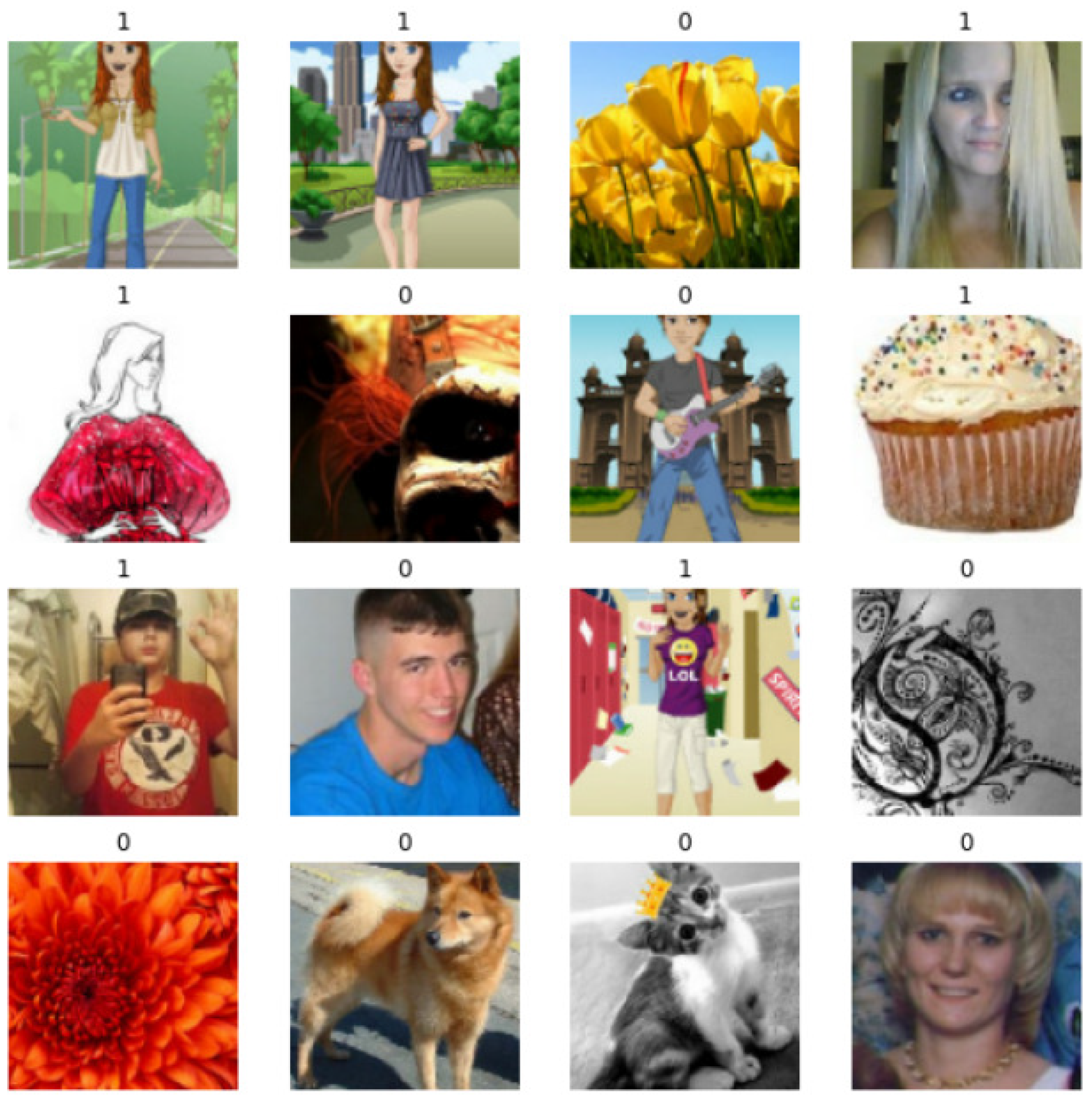Lastly, the feed-forward attention mechanism of [27] was able to discover the most informative and reliable parts of given faces for improving age and gender classification. In the case of Yahoo! Answers, members use assorted images on their profiles, including avatars, landscapes, objects, shields, flags and real faces of course. This wide variety together with their small size make the recognition of age based on this modality a very challenging task.

All in all, automatic age prediction across cQA members is a largely unexplored area of research. This work pioneers the efforts in that direction by dissecting the main challenges across different modalities, and by presenting an effective way of alleviating two of them (texts and meta-data), independently.

3. Dataset

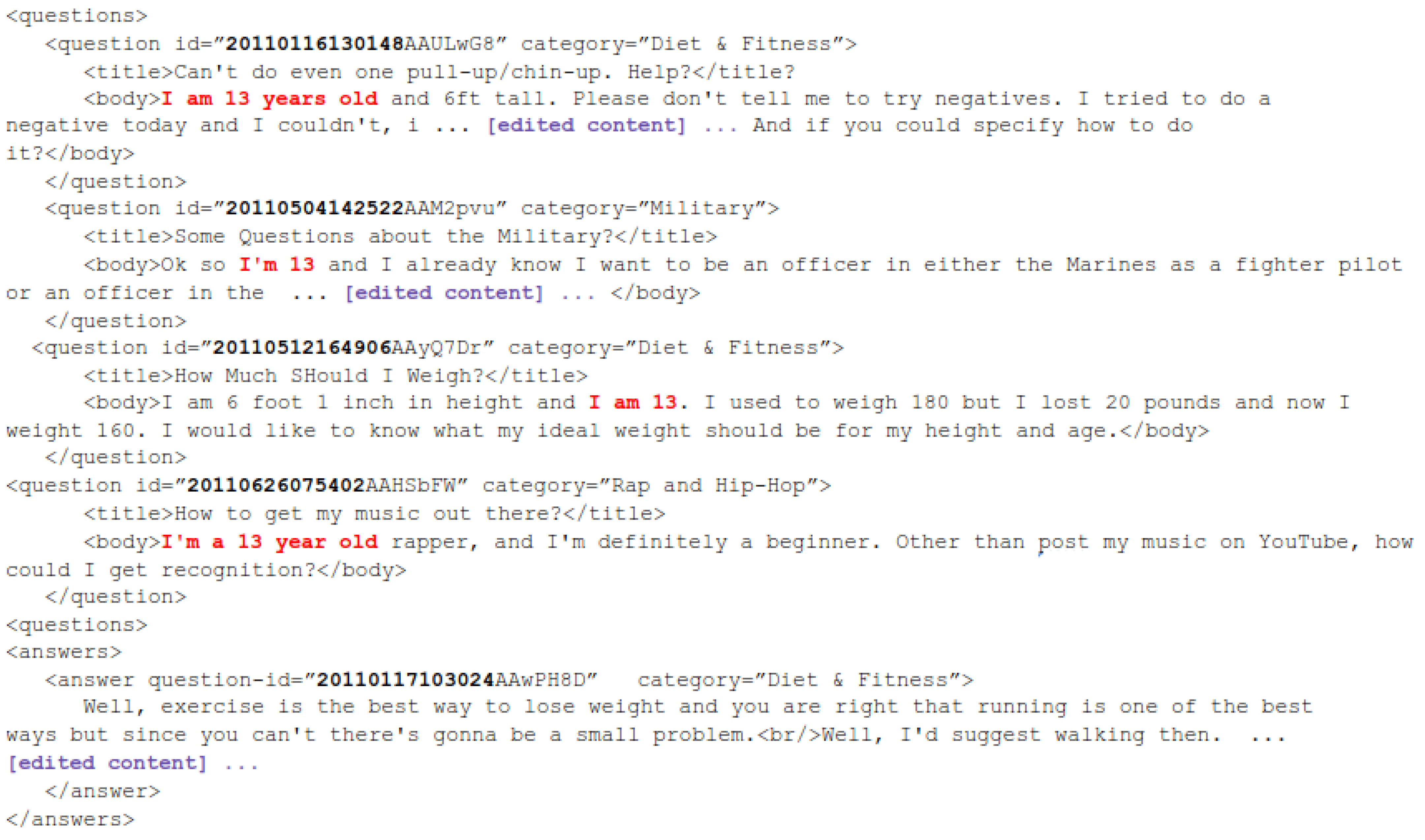
In order to fetch user profiles (see Figure 1) and question-answers pages (see Figure 2) from Yahoo! Answers, we took advantage of the web scraper implemented in [28], which ran for around three years (September 2015–2018). As a result, about 53 million of question-answers pages were retrieved, wherefrom all question titles, bodies and answers were extracted accordingly; and in the same manner, ca. 12 million profile pages were downloaded. From these pages, we extracted self-descriptions, images and lists of questions. We then singled out all textual content written predominantly in English by means of a language detector (https://code.google.com/archive/p/language-detection/ (accessed on 1 February 2021)). See a sample record in Figure 3.

Our automatic annotation process starts off by searching for valid putative birth years (1910–2008) and ages (10–99) at the paragraph level. Additionally, correspondingly, all mismatching paragraphs are eliminated. The next step consists of splitting the selected paragraphs into sentences via CoreNLP (http://stanfordnlp.github.io/CoreNLP/ (accessed on 1 February 2021)). For each sentence, we verified if it starts with any of following three surface patterns: (a) [I am|I m|I’m|Im|I turned] [|an|now|only|age|turning] NUMBER; (b) I was born [in|on] [DATE|YEAR]; and (c) My age is NUMBER.

We conducted a case-insensitive alignment, and checked as to whether or not after the number we could find an occurrence of a unit such as kg and mg, or a period of time such as weeks or days. In so doing, we made sure that these matched numbers did not correspond to commonly used metrics/units explicitly mentioned in the text. Every time these alignments failed, we carried out a POS-based analysis by basically ensuring that: (a) there was only one pronoun and no additional verb before the first identified number/year; and (b) there was no negation before the first number/year.

On the whole, 657,805 users were automatically labelled, and all sentences used to determine their age where removed from the respective texts. Note that, from these members, only 219,626 (33.39%) used a non-default profile image.

Table 1. Definitions and distributions of the different age clusters across the United States and our collection.

Generation	Birth Years	USA (Million)	Texts/Metadata	Profile Images
Gen Z	1995–2008	74	321,912 (48.94%)	82,162 (37.40%)
Gen Y	1980–1994	73	276,493 (42.03%)	110,463 (50.28%)
Gen X	1965–1979	82	37,301 (5.67%)	17,330 (7.89%)
Baby Boomers	1944–1964	76	17,705 (2.69%)	8083 (3.68%)
Matures	1910–1943	-	4394 (0.67%)	1645 (0.75%)
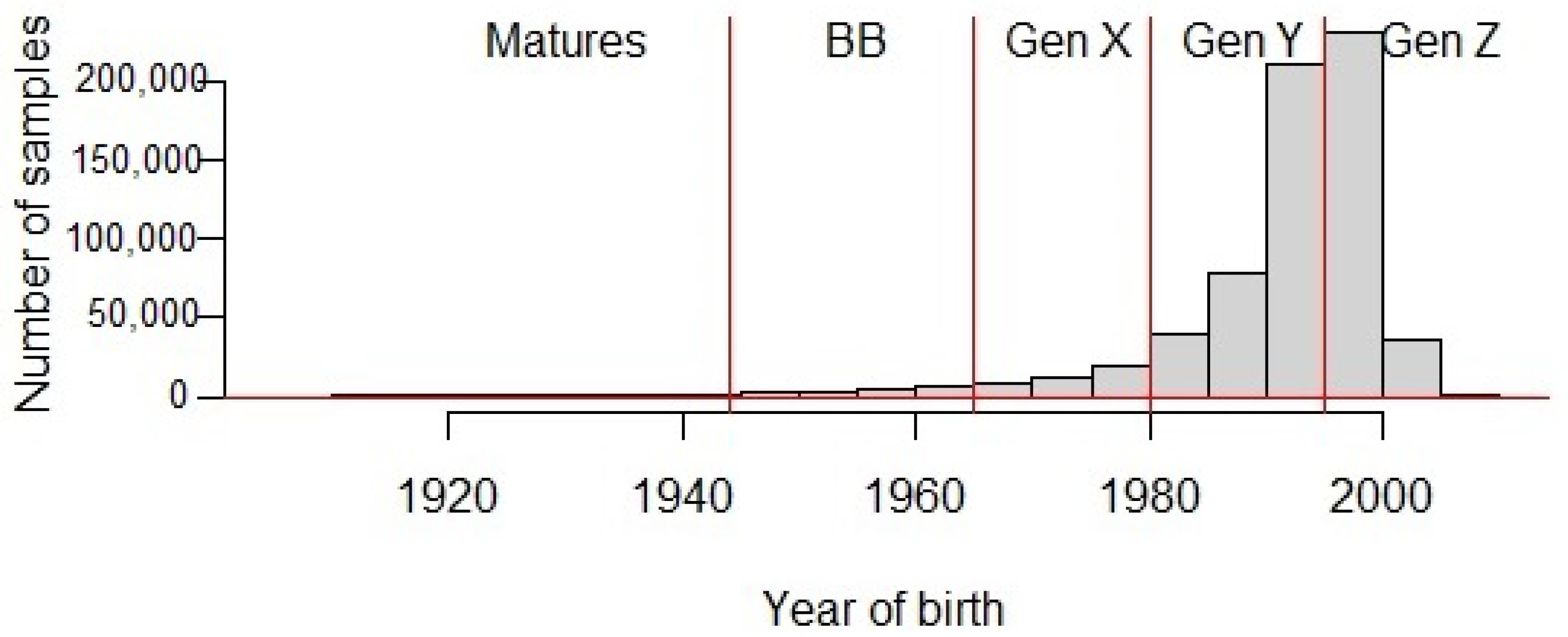
Total			657,805	219,683

gives an intuition about the age distribution observed within our corpus across both modalities (i.e., texts/metadata and images). As a means of facilitating this comparison, samples were grouped by following the theory of William Strauss and Neil Howe [29]. This is premised on the proposition that each generation belongs to one of four classes, and that these classes repeat sequentially in a fixed pattern. By virtue of these descriptors, five distinct cohorts were identified: Matures, Baby Boomers, Generation X-ers, Millennials/Gen Y-ers and iGen/Gen Z-ers (https://www.kasasa.com/articles/generations/gen-x-gen-y-gen-z (accessed on 1 February 2021)). It is worth mentioning there that people born earlier than 1944 became members of the additional cluster "Matures."

For experimental purposes, these samples were randomly divided into 394,745 training (60%), 131,519 testing (20%) and 131,541 evaluation (20%) instances in such a way that we ensured similar distributions of all five target categories across these three splits (see Table 1). Additionally, as for images, the distribution was as follows: 131,682 (59.94%) training, 43,972 (20.02%) testing and 44,029 (20.04%) evaluation. It is worth stressing here that we kept full consistency between text and image splits; that is to say, each community peer was used for the same purpose (i.e., training, testing or evaluation) for both sets (i.e., texts and images).

In summary, our corpus unveils that, like other online platforms, older people continue to trail both Gen Z and Millenials in the adoption of online cQA platforms, especially Yahoo! Answers (see Figure 4). As a natural consequence, the data are skewed; this means most of the data are on the right-hand side of the graph (younger generations) and the long skinny tail extends to the left (mature people). More specifically, the entropy of the text set is 1.4536, whereas this value is 2.322 for perfectly balanced classes. Note also that about 50% of the text samples belong to the youngest generation (Gen Z), and ca. 50% of the image samples are members of Gen Y; and in this set, the entropy is 1.5447, indicating a higher uncertainty in the distribution of its prior probabilities. Lastly, it worth stressing that differences in age distributions might also be sharp across distinct modalities (i.e., texts, images and metadata).

4. Text Analysis

The trailing discussed in the previous section brings about an under-representation that has a marked and harmful influence on the demographic analysis and on machine learning models, especially supervised approaches. In our study, we cast age prediction as a classification task via capitalizing, in the first place, on the segmentation provided by Strauss and Howe (see Table 1). Based on these divisions, we quantify the significance of this repercussion on the following state-of-the-art neural network classification models built solely on textual inputs:

• FastText (https://fasttext.cc/docs/en/support.html (accessed on 1 February 2021)): It is a simple and efficient library for learning word embeddings and text classification, rivaling deep learning classifiers in terms of accuracy, but many orders of magnitude faster. This model is a simple shallow neural network with only one layer. The bag-of-words representation of the text is first fed into a lookup layer, where the embeddings are retrieved for every single word. It constructs averaged n-gram text representations, which are fed to a linear classifier afterwards (multinomial logistic regression). A softmax layer is utilized for obtaining a probability distribution over pre-defined classes, and stochastic gradient descent is combined with a linearly decaying learning rate for training [30,31].
• Deep Neural Networks (https://www.tensorflow.org/ (accessed on 1 February 2021)): We capitalized with four word-level text classification strategies implemented in Tensorflow (https://github.com/dongjun-Lee/text-classification-models-tf (accessed on 1 February 2021)): CNN [32], bidirectional RNN (B-RNN), attention-based bidirectional RNN [33] and RCNN [34].

In order to reduce the bias in our assessments, or in other words, to consider distinct plausible applications, we took advantage of three different metrics in our evaluations that are widely used across several text-oriented multi-class settings: Accuracy, MRR (mean reciprocal rank) and macro-F1-score. A brief description of each metricfollows:

• Accuracy: the fraction of instances that were correctly predicted by a given model.
• Mean reciprocal rank (MRR): The multiplicative inverse of the position in the confidence ranking of the first correct label [35]. Accordingly, the MRR is the average of the reciprocal ranks of the predictions output for an array of community members.
• Macro-averaged F1-score, or macro-F1 in short: this combines the per-class F1-scores into a single number by computing their simple arithmetic mean. This metric is more influenced by the performance on rare categories [36].

Table 2. Accuracy (%)/MRR/macro-F1-score achieved by the for the different age cohort distributions (test set).

	Strauss & Howe	Reduced Strauss & Howe	cso.ie	Ten Year Groups
FastText	70.30/0.8388/0.3444	71.79/0.8530/0.6350	70.18/0.8398/0.3343	66.73/0.8095/0.2172
CNN	64.66/0.8079/0.2696	62.24/0.8002/0.4361	64.87/0.8089/0.2752	65.52/0.8126/0.1978
RCNN	66.61/0.8194/0.2371	67.77/0.8311/0.5752	66.55/0.8190/0.2221	66.87/0.8207/0.2372
Bi-RNN	67.23/0.8232/0.2337	68.10/0.8334/0.5639	67.64/0.8254/0.2230	67.11/0.8225/0.2387
Attention RNN	67.92/0.8268/0.2447	68.08/0.8332/0.5924	67.75/0.8259/0.2401	67.68/0.8254/0.2443
Average	67.34/0.8232/0.2659	67.60/0.8302/0.5605	67.40/0.8238/0.2589	66.78/0.8181/0.2270

underscores the outcomes accomplished by each configuration of neural network learner and metric. Fundamentally, our experiments point to the following findings:

• Although Accuracy and MRR are, by and large, fairly high for a five-class task (the former over 64% and the latter over 0.8), macro-F1 is quite low (between 0.24 and 0.35). Both things together indicate that trained models are likely to be almost "two-sided"; in other words, they mainly specialize in discriminating between the two largest age cohorts (i.e., Gen Y and Z).
• A shallow neural network (FastText) outperformed much more complex architectures by a considerable margin regardless of the metric in consideration. It assigns, for instance, the correct age group to 2.38% more members than its closest rival (Attention RNNs). This result suggests that more research efforts should go into tackling imbalances produced by trailing than into designing more complex architectures.
• However, more importantly, FastText accomplished a marked improvement in terms of macro-F1 (over 27%), meaning that it performed better across the five cohorts on average, and this entails that it was relatively successful at coping with the data imbalance. It is worth highlighting here that this a desired, but not easy to achieve result. See, for instance, the outcomes of CNN; this deep neural network improved in terms of this metric, but its performance diminished in relation to Accuracy and MRR.

In summary, the best configuration finished with a fairly high performance, pointing not only to the fact that age groups can be effectively identified from their textual inputs, but also that this can be done efficiently, since FastText can run under very limited resources. However, our figures indicate that class imbalances manifested across age groups seriously hurt the learning of text-based neural network models.

The next step in our study was testing different age cohort descriptors; this way we could conduct experiments with different numbers of classes and distributions. For this purpose, we accounted for the following three additional segmentations:

• Reduced Strauss and Howe: We amalgamated the three oldest and under-represented groups into only one cluster named "Matures" (see

  Table 3. Different age cohort descriptors (reduced Strauss and Howe).

  Group	Birth Years	Texts/Metadata
  GEN Z	1995–2008	321,912 (48.94%)
  GEN Y	1980–1994	276,493 (42.03%)
  Matures	1910–1979	59,400 (9.03%)
  Total		657,805

  ). We devised this distribution based on our prior empirical observations. More precisely, our intuition is that having only one larger, but still under-represented group would lighten the burden on learning model parameters, resulting in fitter models.
• cso.ie: We took advantage of the grouping utilized for the 2016 Irish census (https://www.cso.ie/en/releasesandpublications/ep/p-cp3oy/cp3/agr/ (accessed on 1 February 2021)) (see

  Table 4. Different age cohort descriptors (distributions).

  cso.ie			Ten Year Groups
  Group	Birth Years	Texts/Metadata	Group	Texts/Metadata
  Primary	2006–2008	212 (0.03%)	1999–2008	103,995 (15,80%)
  Secondary	2000–2005	62,804 (9.55%)	1989–1998	411,574 (62,56%)
  Young adults	1994–1999	309,002 (46.97%)	1979–1988	87,189 (13,25%)
  Matures	1954–1993	275,639 (41.91%)	1969–1978	26,496 (4,03%)
  Adults	1910–1953	10,148 (1.54%)	1959–1968	13,768 (2,09%)
  			1949–1958	7988 (1,21%)
  			1910–1948	6795 (1,03%)
  Total		657,805		657,805

  ). The underlying reason behind this choice is that its two largest cohorts are slightly smaller than the other considered distributions, summing up to a total of 88.88%. Like Strauss and Howe, it divides people into five clusters, but unlike Strauss and Howe, these divisions are substantially more uneven.
• Ten year groups: We also made allowances for a traditional ten year segmentation (see Table 4). This kind of division is utilized across several sorts of demographic analyses, and in our case, it produces an extremely imbalanced prior distribution encompassing seven age groups. More specifically, the 1989–1998 cluster comprises 62.56% of the members.

Table 2 juxtaposes the performance reaped by each neural network learner when considering these three segmentations. In this light of these outcomes, we conclude:

• Interestingly enough, FastText outclassed all deep architectures by a clear margin every time community fellows were represented by means of three or five cohorts. This superiority was also seen regardless the metric used for the assessment. However, on the flip side, its competitiveness notoriously worsened when members were modeled by means of ten groups.
• Independently of the metric, the larger the number of age groups, the larger the decrease in average performance. In particular, when targeting ten clusters, neural networks models finished with an accuracy between 65.52% and 67.68%. These values are only 3–5% over the majority class baseline, which scored an accuracy of 62.56%. On the other hand, when aiming at five cohorts, the majority baselines scored accuracies of 46.97% and 48.94%, and the values achieved by the deep networks range from 64.66% to 67.92% (accuracy). All these things considered, learning was less effective in the presence of greater class imbalances and when increasing the number of age cohorts.
• Independently of the metric, FastText and most of deep learning methods accomplished better performance when community members were represented via three age cohorts. While this might seem self-evident due to the fact that the average is computed on a lower number of unrepresented classes, it is also pertinent to consider its increase in accuracy. That is to say, there was a noticeably higher rate of correct predictions.

To sum up, clustering all under-representing age cohorts into one group showed to be an efficient way of casting age prediction as a classification task. In particular, using three groups lessens the distortion attributed to data imbalances. Needless to say, our empirical results also highlight the efficiency of FastText as a strong, efficient and simple baseline for age classification.

Another way of tackling data imbalances is adjusting its class distribution. To illustrate, one common strategy is removing some training instances. This practice is supported by the debated Newport’s "less is more" hypothesis [37]; i.e., child language acquisition is aided, rather than hindered, by limited cognitive resources. In the case of supervised machine learning, this means that model generalization can be hurt by an excessive amount of training material. This can happen, for example, if there is an over-representation of some traits that typify a class.

In curriculum learning [38], a learning plan is devised by ranking samples based on carefully chosen and thoughtfully organized difficulty metrics. In that vein, the work of [39] proposed a battery of heuristics for sorting the training samples to be fed to their learning algorithm. Broadly speaking, these heuristics select the next element within the training material that will be adjoined to the array of instances already presented for learning. Since feeding one example at a time is computationally expensive, one can gain a significant speed advantage by picking samples in batches. In practice, this results in a small loss in terms of accuracy. Following the spirit of this kind of technique, we designed a greedy algorithm (age-batched greedy curriculum learning) that systematically and incrementally creates sample batches according to birth years, and feeds FastText with these instances afterwards.

At length, age-batched greedy curriculum learning, or AGCL for short, starts with three empty bags of batches: one for each age cohort in accordance with the reduced Strauss and Howe segmentation (see Table 3). Let these bags be: ${\Phi }_Z$ (Gen Z), ${\Phi }_Y$ (Gen Y) and ${\Phi }_M$ (Matures). After each iteration, this algorithm adds the combination of batches that performs the best (i.e., single, pair or triplet). In order to determine this tuple, this procedure tests each non-selected combination of zero or one batch from each cohort together with all the batches already contained in these three bags (see this flow on

Table 5. Curriculum discovered by AGCL. Results are shown in terms of macro-F1-score on the evaluation set (Eval). This table also highlights the percentage of the data (from the 394,745 training instances) used for building each model (Total). It additionally displays its respective class distribution (%) and entropy.

	Batch(es) Added				Data Distribution
Step	Matures(${\mathbf{\Phi }}_{\mathit{M}}$)	Gen Y(${\mathbf{\Phi }}_{\mathit{Y}}$)	Gen Z(${\mathbf{\Phi }}_{\mathit{Z}}$)	Eval	Matures	Gen Y	Gen Z	Total(%)	Entropy
1	1978	1994	1997	0.5570	3.71	46.01	50.28	16.55	0.358
2	1977		2007	0.6104	6.78	44.53	48.69	17.10	0.388
3	1979	1990	1999	0.6323	6.66	40.08	53.26	27.33	0.383
4	1970		2002	0.6421	7.30	37.45	55.25	29.25	0.385
5	1964		2003	0.6478	7.68	36.07	56.24	30.37	0.386
6	1976	1988	2004	0.6523	8.34	39.47	52.19	33.50	0.397
7	1973		2006	0.6557	9.30	39.02	51.68	33.88	0.404
8	1966		2005	0.6583	9.90	38.60	51.51	34.25	0.407
9	1972	1989	2000	0.6591	9.06	38.43	52.51	41.32	0.401
10	1968			0.6625	9.68	38.17	52.16	41.61	0.405
11	1975	1993	1998	0.6649	7.90	39.82	52.28	56.17	0.394
12	1957			0.6671	8.18	39.69	52.12	56.34	0.396
13	1962		2001	0.6679	8.17	37.92	53.91	58.98	0.393
14	1974			0.6697	8.73	37.69	53.58	59.34	0.397
15	1951	1984		0.6709	8.71	38.95	52.34	60.75	0.399

). The algorithm stops when it is impossible to add a tuple that enhances the performance. As for the metric and learning approaches, macro-F1 score and FastText were used, respectively. It is worth underscoring here that we opted for looking into this metric, since our previous experiments indicated that this is seriously challenged by class imbalances. Note also that the evaluation set remained unchanged during the entire iterative process; i.e., it always comprised all 131,541 samples sketched in Section 3.

The outcome of AGCL is a sequence of inputs ordered by their power of generalization and informativeness regarding the three categories that leads to more resource-efficient learning (see Table 5). In the first iteration, this curriculum determines the tuple (up to three age batches) that makes both a broader generalization and a clearer separation of the three groups. In our case, the years 1978, 1994 and 1997 were added to ${\Phi }_M$, ${\Phi }_Y$ and ${\Phi }_Z$, respectively. Interestingly enough, AGCL singled out batches that were alongside both category borderlines; i.e., 1978 is in the vicinity of the 1979–1980 border, and 1994 and 1997 are near to the 1994–1995 border. We interpret this as an attempt at finding effective separations between classes by discovering fine-grain discriminative characteristics between pairs of consecutive generations—that is to say, by finding out distinctive traits that signal the shift from one generation to the next one. Naturally, and as a means of gaining generalization power, the algorithm prefers to choose two batches from the 1994–1995 border, instead of the 1979–1980 border, due to their bigger share of the dataset.

In the second iteration, AGCL selected a pair of batches instead of a triplet (i.e., 1977 and 2007). We view this selection as a confirmation of the initial trend. In other words, examples born in the year 2007 are likely to correspond to members bearing the sharpest differences to any individual born in 1994 or earlier. Although this array of individuals is very small (19 samples), they aided in enriching the model with very discriminative features, while at the same time keeping their relative share of the training input virtually intact. On the other hand, the addition of 3585 mature members born in 1977 aimed mainly at enhancing generalization by counterbalancing the representations of the other two groups in terms of number of instances (see data distribution in Table 5).

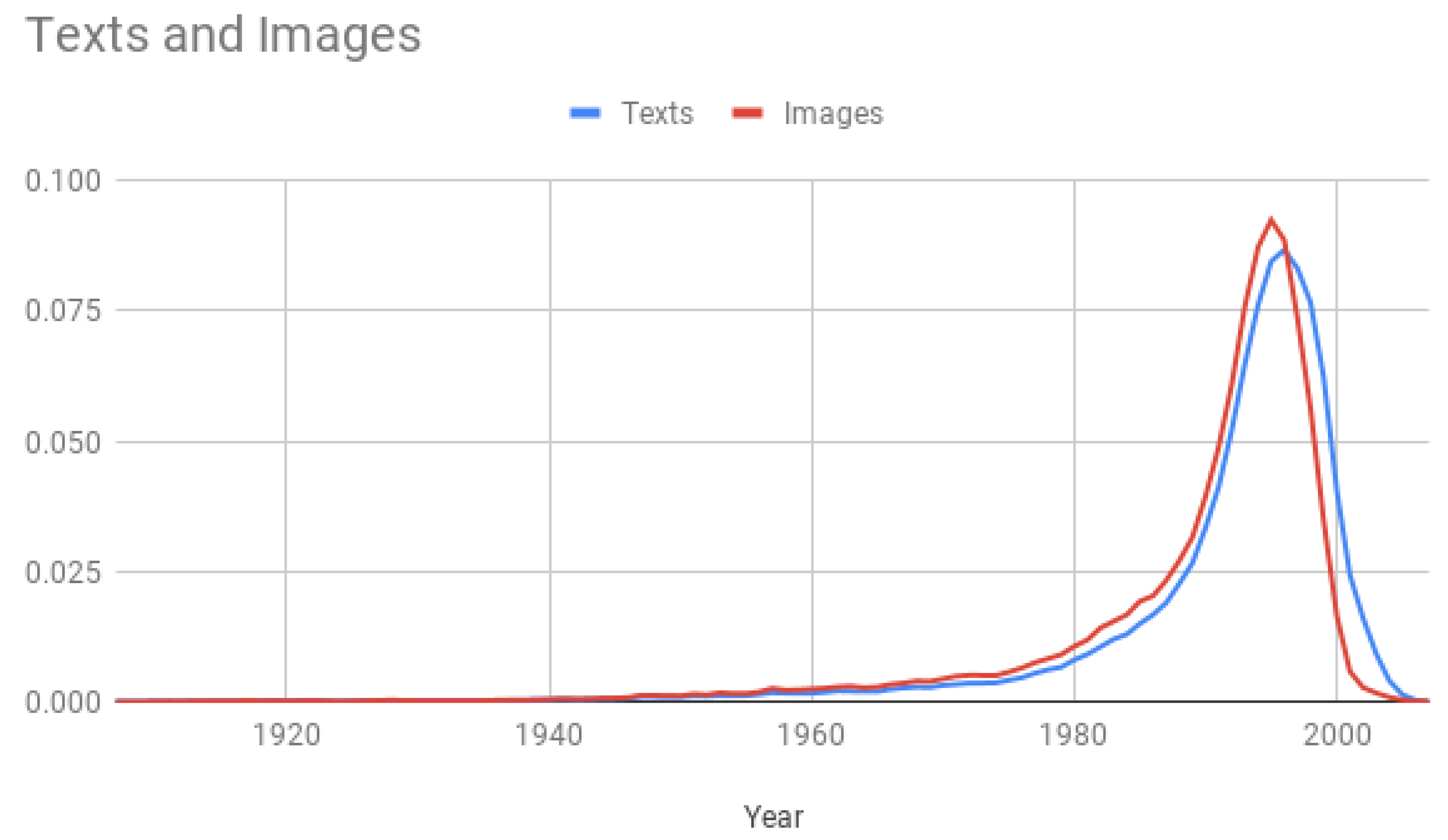
In summary, the goal at the beginning of learning plan is two-fold: (a) adding a large number of instances distilled from the under-represented cohort (i.e., Matures); and (b) finding out attributes informative of the two largest groups (i.e., Gen Y and Z). Note also that the former goal keeps going until the seventh iteration, where six out of the seven batches picked by AGCL belong to community fellows born in the 70s (cf. Figure 4).

Furthermore, one of the primary focuses of attention during the last iterations was harvesting salient attributes from the Matures. In so doing, ACGL chose batches from this group that were small and far from the 1979–1980 border. With its last additions, AGCL reaps modest improvements via bringing specifics into the model. In a nutshell, AGCL devises the curriculum by sorting age batches in consonance with their contributions to the learning process from more general to more specific features. In quantitative terms, our experiments yielded the following results:

• Overall, AGCL finished with macro-F1-scores of 0.6709 and 0.6660 on the evaluation and test sets, respectively. Conversely, the best model constructed on top of the entire training material achieved on the test set a score of 0.6350. This means an improvement of 3.94% (0.6350→0.6660) caused by smartly reducing the training set by 40% (cf. Table 2).
• More precisely, AGCL needed 60.75% of the training set in order to accomplish the mentioned score of 0.6660. Specifically, this subset encompassed 58.52%, 56.29% and 64.98% of the available training instances for Matures, Gen Y and Gen Z, respectively. On the one hand, Gen Z increased its share of the data used for building the model from 48.94% to 52.34%; on the other hand, its two largest batches were not chosen (1995–1996). Why? We deem this to be a result of trying to capture a wider variety of informative traits that seem to be spread all throughout the generation. Additionally, presumably, the two largest batches share a lot of commonalities with both the previous generations and the instances selected from their own cohorts.
• In juxtaposition, AGCL singled out few from the batches available for Gen Y, and therefore took a smaller fraction of the training material; i.e., its share diminished from 42.03% to 38.95%. Given that fewer data are required for their accurate representation, we conclude that community members belonging to this generation are much more homogeneous (see Figure 5).
• If we pay attention to the selections for the Mature cluster, we discover an additional piece of information on how AGCL is increasing the diversity of the discriminative features across the training set. From 1962 to 1972, AGCL integrated solely even years into the model (dismissing odd years). We perceive this skipping pattern as an indication of prioritizing trait diversity over enlarging its share of the training set (see Figure 5). Note here that batches systematically decrease in size in consonance with their birth year (cf. Figure 4).

In conclusion, our findings point out to the fact that the distribution of classes should be in tandem with the diversity of their members. Put differently, it is not a matter of gathering an equal amount of instances of each class, but of having enough samples for covering the diversity of each category. It is here where generational trailing has its greater negative impact, because it makes building this collection for older members much harder. It is crystal clear that the unbalance discovered by AGCL stems from this and another two factors: (a) the larger amount of diverse young people coming from different walks of life that have adopted the use of online platforms such as Yahoo! Answers; and (b) although Gen Y is a massive cohort, it is much more heterogeneous, and hence it can be represented by a comparatively smaller set of instances.

5. Meta-Data

In order to dig deeper into the meta-data view, we capitalized on the training material used for our text analysis (see also Section 3), namely, the 394,745 training instances (due to computational limitations (Intel Corei5 CPU), it was infeasible to run the R software on the entire dataset), for extracting 95 meta-data non-negative integer variables. Most of these elements correspond to frequency counts (see variable descriptors on

Table A1. Descriptions of variables (questions or answers).

Variable	Meaning
birth.year	Year of birth
1st.level.cat.highest.frequency	Frequency count of most recurrent 1st level categories
1st.level.cat.highest.frequent	Most recurrent 1st level categories
1st.level.cat.unique	Number of different 1st level categories
2nd.level.cat.highest.frequency	Frequency count of most recurrent 2nd level categories
2nd.level.cat.highest.frequent	Most recurrent 2nd level categories
2nd.level.cat.unique	Number of different 2nd level categories
3rd.level.cat.highest.frequency	Frequency count of most recurrent 3rd level categories
3rd.level.cat.highest.frequent	Most recurrent 3rd level categories
3rd.level.cat.unique	Number of different 3rd level categories
ampm.marker.highest.frequency	Frequency count of most recurrent am/pm timestamp
ampm.marker.highest.frequent	Most recurrent (none, AM or PM)
ampm.marker.unique	0, 1 or 2 (none, AM and/or PM)
day.month.highest.frequency	Frequency count of most recurrent day in the month (1–31)
day.month.highest.frequent	Most recurrent day in the month
day.month.unique	Number of different days in the month
day.week.highest.frequency	Frequency count of most recurrent day in the week (1–7)
day.week.highest.frequent	Most recurrent day in the week
day.week.unique	Number of different days in the week
day.year.highest.frequency	Frequency count of most recurrent days in the year (1–365)
day.year.highest.frequent	Most recurrent day in the year
day.year.unique	Number of different days in the year
hour.day.highest.frequency	Frequency count of most recurrent hour (0–23)
hour.day.highest.frequent	Most recurrent hour in the day
hour.day.unique	Number of different hours in the day
maxYear	Latest year within the timestamps
minYear	Earliest year within the timestamps
minute.hour.highest.frequency	Frequency count of most recurrent minute (0–59)
minute.hour.highest.frequent	Most recurrent minute
minute.hour.unique	Number of different minutes in the hour
month.year.highest.frequency	Frequency count of most recurrent month in the year (1–12)
month.year.highest.frequent	Most recurrent month in the year
month.year.unique"	Number of different month in the year
second.minute.highest.frequency	Frequency count of most recurrent second (0–59)
second.minute.highest.frequent	Most recurrent second
second.minute.unique	Number of different seconds
week.month.highest.frequency	Frequency count of most recurrent week in a month (1–5)
week.month.highest.frequent	Most recurrent week in the month
week.month.unique	Number of different weeks in the month
week.year.highest.frequency	Frequency count of most recurrent week in a year (1–52)
week.year.highest.frequent	Most recurrent week in a year
week.year.unique	Number of different weeks in the year
year.highest.frequency	Frequency count of most recurrent year (2006–2018)
year.highest.frequent	Most recurrent year
year.unique	Number of different years

and

Table A2. Descriptions of variables (global).

Variable	Meaning
endActYear	the year when the user finished his activity in the community
initActYear	the year when the user started his activity in the community
yearsActive	Number of years of activity in the community
no.answers	Number of posted answers
no.best.answers	Number of posted best answers
no.questions	Number of posted questions

on Appendix A).

The methodology of analysis consisted of four different steps: (1) we cleared the data by detecting and eliminating anomalous values; (2) as a means of reducing the number of dimensions, we applied principal component analysis (PCA) for identifying the subset that largely contributed to the total variability; (3) we applied a correlation function for determining the groups of variables that exhibited the highest correlations with the different age cohorts; and finally, (4) we implemented random forest classifiers to distinguish between the two youngest age clusters (i.e., GenZ and GenY). As a result, we discovered the most informative variables.

First, graphical tools and summary statistics have been used for detecting anomalous values, which were eliminated accordingly. Anomalous values stem from several reasons, including errors during the pre-processing of the corpus. Next, PCA was performed on the clean material. Note that PCA is a technique aimed at describing a multidimensional data, using a smaller number of uncorrelated variables (the principal components) that incorporate as much information from the of the original dataset as possible (see Reference [40] and the references therein). 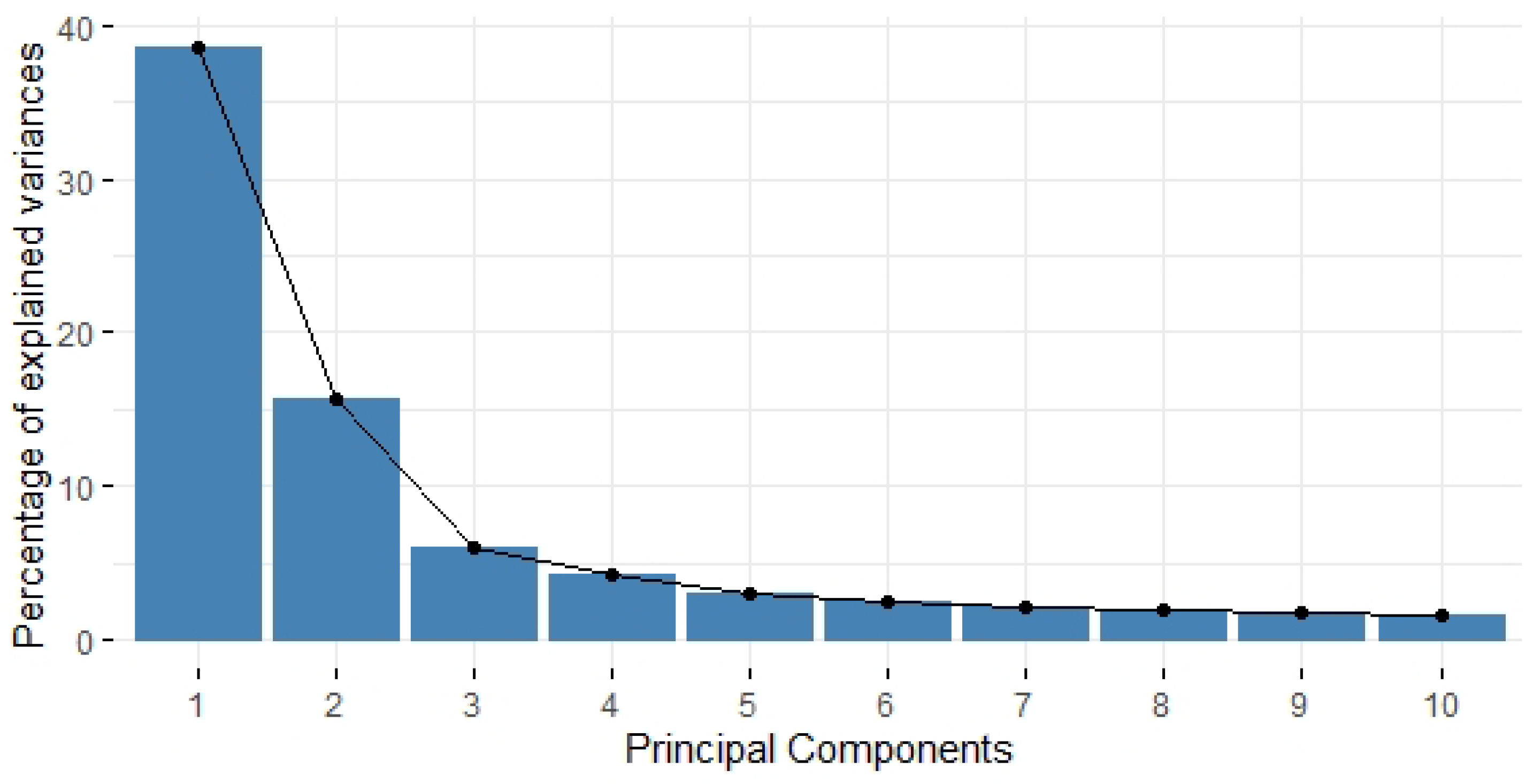(We used the implementation from the FactoMineR package [41] in R software [42]). 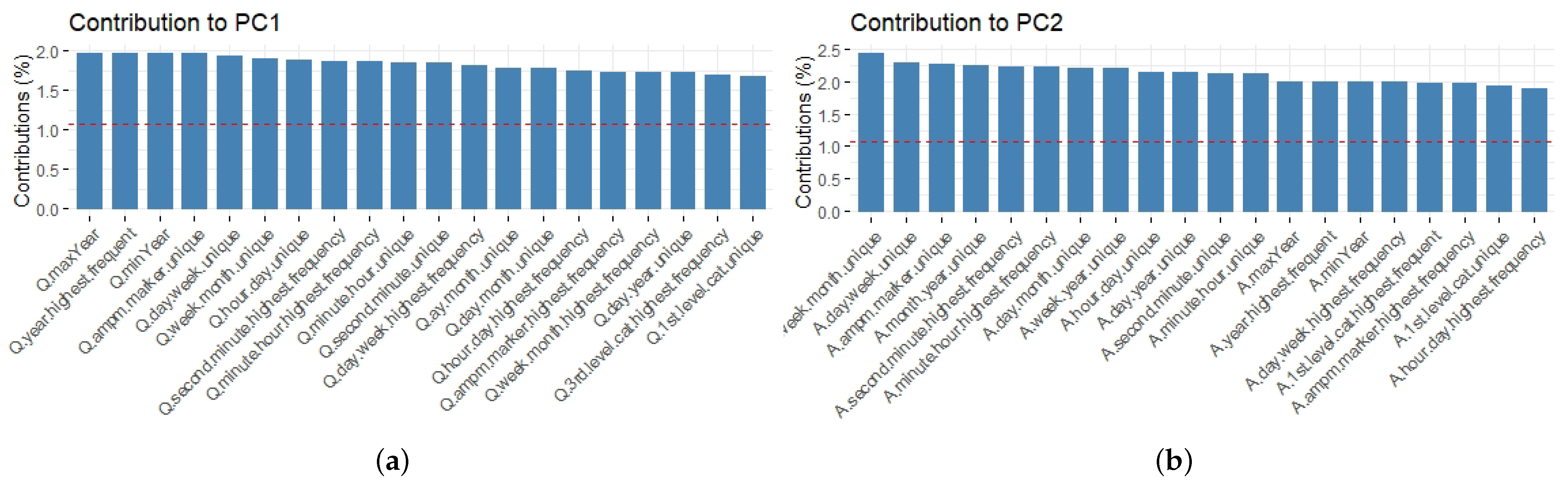In light of this analysis, we found out that the first two principal components take into account 54.26% of the total variance (Figure 6). It additionally reveals the contributions of the first 20 variables to components 1 and 2, which are represented in Figure 7a,b, respectively. Although the differences among contributions are very small, variables harvested from questions seem to help the first component more. However, given that almost all variables provide a significant variability, it is not possible to select a few elements which represent most of the variance of the entire data set.

Furthermore, correlation analysis unveils that age (year of birth) is more correlated with variables distilled from questions than from answers. To be more precise, Figure 8 highlights their Pearson correlation coefficients. From these results, we can conclude that question variables (from 51 to 94 ) seem to be better age predictors than their counterparts extracted from answers (from 2 to 44). The first correlation equal to one indicates that the correlation of the first variable is with itself. However, the highest correlations are with variables 45 and 46; those are the years that the members started and ended their activities, respectively. Additionally, from Figure 8, it emerges that answers are negatively correlated with the year of birth, while questions are positively correlated.

Our last analysis consisted of applying random forest classifiers (introduced by [43]) for identifying which variables are more informative of the different age cohorts. For this, we grouped the data into five age cohorts according to the definitions in Table 1. However, since these groups are highly unbalanced (as shown in Figure 9 and Table 1), we only considered the two youngest clusters (i.e., Gen Y and Gen Z) for this analysis. Given the aforementioned computational restrictions, the training data were randomly split into 75% and 25% for the training and testing, respectively.

By using $n=500$ trees, RF classifiers obtained an accuracy of 0.74, a sensitivity of 0.7794 and a specificity of 0.7149. The performance significantly improved when RF was implemented by excluding samples corresponding to birth years close to the border. For example, by considering from Gen Z all the individuals who were born between 2000 and 2008 and from Gen Y all members born between 1985 and 1990, the accuracy increased to 0.9248, and the sensitivity and specificity were 0.9486 and 0.9020, respectively. This means that individuals close to the border are very similar, and hence difficult to classify.

Overall, RF classifiers singled out eight discriminative year-based variables (see

Table 6. The top 20 most important variables (out of 95). The values are scaled between 0 and 100. Q, A and G denote elements extracted from questions, answers and global (combines all information), respectively (see variable descriptors on Appendix A).

Ranking	Source	Variable	Importance
1	G	initActYear	100.00
2	G	endActYear	99.08
3	Q	minYear	85.43
4	Q	year.highest.frequent	85.03
5	Q	maxYear	83.56
6	A	year.highest.frequent	58.74
7	A	minYear	57.07
8	A	maxYear	57.04
9	A	3rd.level.cat.highest.frequency	35.95
10	A	1st.level.cat.highest.frequency	35.56
11	A	ampm.marker.highest.frequency	34.16
12	A	minute.hour.unique	34.11
13	A	second.minute.unique	33.77
14	G	no. questions	33.61
15	A	day.month.unique	33.56
16	A	day.month.unique	33.56
17	A	day.year.unique	33.48
18	A	2nd.level.cat.highest.frequency	33.41
19	A	month.year.highest.frequency	32.83
20	A	year.highest.frequency	32.48

): (1) when the user started his/her activity in the community; (2) when his/her activity finished; (3) when he/she was prompted with the first question; (4) when he/she asked more questions; (5) when he/she posted the last question; (6) when he/she answered more questions; (7) when his/her first answer was published; and (8) when his/her last answer was posted. Since we used the implementation of RF classifiers provided by the caret package of R software, the importance of variables was evaluated using statistical non-parametric methods included in its tt varImp function.

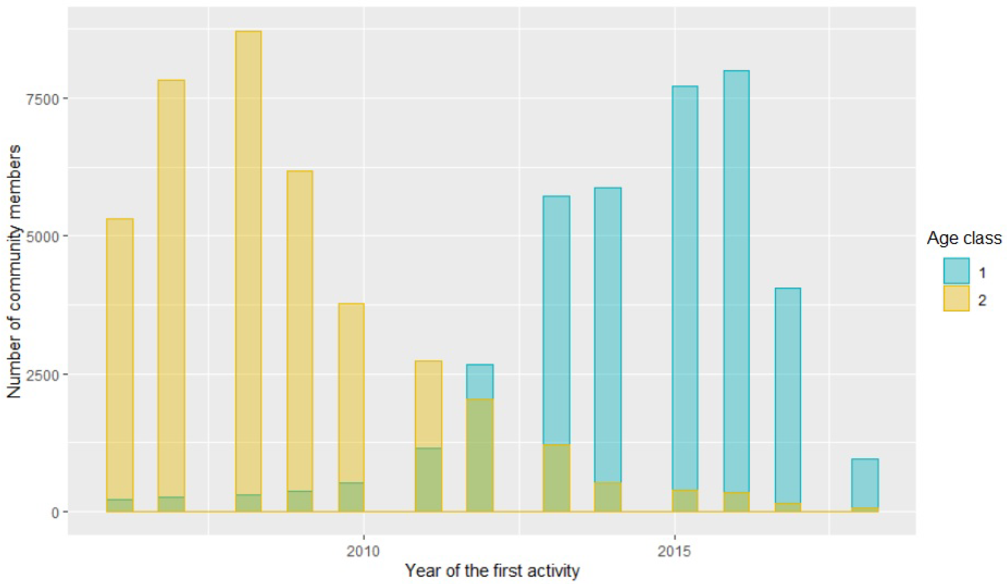
If we observe the histogram plot corresponding to the top selected variable (considering $N=77,018$ samples), that is to say the element denoting the year when a community member starts his/her activity in the site, we find a different behavior for Gen Z (class 1) with respect to Gen Y (class 2), which allows one to improve the classification rate (see Figure 10).

From all these analyses, we can conclude that the years of starting and ending activities in the social network are important variables for estimating the age of the users. Additionally, it seems that the age is more correlated to variables related to questions than to answers, allowing a better predictive ability. Finally, the age cohort prediction significantly improves when no continuous classes are considered, suggesting a new definition of their limits.

6. Image Analysis

Computer vision seeks to give computers human capabilities for pattern recognition from images and it is an essential part of the Internet of Things [44], robotics [45] and human brain interfaces [46]. Despite the progress made, research in this area is still evolving. Needless to say, visuals differ in textual patterns, and thus they can work together as complementary sources of effective features for any given prediction task that has both modalities at hand.

Like textual patterns, the complexities of visual patterns are best captured by machine learning methods. In this case, machine learning algorithms are based on finding the underlying relationship in the image information and thus making decisions without requiring explicit instructions. Multiple classical approaches applied to artificial vision have been considered [47,48]. Similarly to texts (see Section 4), convolutional neural networks [49] has shown great potential in tasks related to computer vision.

Experimentally, deep variants of CNNs are some of the best techniques for recognizing image content and perform effectively in tasks such as segmentation, classification and detection [50]. Even this type of neural network is being used by companies such as Google, Microsoft and Facebook [51], which have developed active research groups seeking continuous improvements in CNN architectures to solve increasingly complex machine vision problems.

The key feature of CNNs is that they can find the correct spatial correlations in the pixel space of images such that neural networks usually can perform visual classification tasks. The typical CNN architecture is based on a sequence of convolutional layers that represent the multiple levels of learning where non-linear processing units and subsampling layers are additionally incorporated. The first network that showed superior performance to the classic alternatives was a deep variant called Alexnet [19]. Currently there are powerful variants of CNNs such as GoogleNet, DenseNet [52] and ResNet [21], among others.

Given these antecedents, an attractive alternative for the recognition of the age group considering the available database is through the use of the images associated with each user, that is, their avatars. We think that the information from image avatars could reveal discriminatory patterns between age groups using deep variants of CNNs. In this section, we will conduct experiments to test this hypothesis. It should be mentioned that in the bibliographic review carried out, there was no precedent for this task.

6.1. Experimental Setting

The dataset consists of the avatar images of the Yahoo! Answers users. Unlike photos found across other social networks, including Flicker (https://www.flickr.com/ (accessed on 1 February 2021)) and Instagram (https://www.instagram.com/ (accessed on 1 February 2021)) (cf. [53,54]), these profile pictures are low resolution; i.e., their size is 128 × 64 pixels on average. The distribution of the classes is given in

Table 7. Number of samples by age group and partition.

Generation	Training Set	Validation Set	Test Set
Gen Z	61,468	20,380	20,391
Gen Y	66,915	22,492	22,509
Gen X	3157	1053	1088
Baby boomers	85	26	27
Matures	17	11	5

:

An inspection of the dataset indicates a huge class imbalance. Due to this imbalance, preliminary experiments on the entire dataset gave poor performance; therefore, we first decided to simplify the learning process by only considering classes Gen Z and Gen Y, since they are the most frequently used to facilitate the task of the visual classifier.

We plan the following experiments to identify the age group of users from their avatar images:

(i). Classification of age groups using original avatars. Original avatars have a high heterogeneity and represent diverse objects such as people, animals, symbols and landscapes. Figure 11 shows random samples of the original avatars.

In this task, multiple standard visual recognition architectures such as convolutional neural networks, VGG [20], ResNet and DenseNet were tested. The convolutional neural network is composed by three convolutional layers and one final fully-connected layer. We used this CNN configuration in the rest of experiments. In the last three neural networks, the transfer learning process was applied based on the weights learned on Imagenet and where the last layer was replaced by a full-connected layer.

(ii). Classification of age groups using virtual human avatars. The original avatars present great diversity, therefore, we decided to test more homogeneous avatars to facilitate the classifier’s work. Specifically, we consider virtual human avatars based on entire bodies. First, we trained a virtual human avatar classifier over a subset of validation data, and then it was applied to the original dataset. Figure 12 shows random samples of virtual human avatars detected.

In this task, we tested convolutional networks with/without data aggregation. The other neural networks were not tested because their performance in the previous task was similar between methods.

6.2. Results

6.2.1. Classification of Age Groups Using Original Avatars

The performances of the neural networks appear to be similar (see

Table 8. Accuracy by age group.

Method	Test (Training)
CNN	59.2% (85.7%)
CNN + data augmentation	58.7% (82.9%)
VGG	59.4% (58.4%)
ResNet	60.6% (60.1%)
DenseNet	57.5% (57.2%)

), either using standard convolutional networks or using more sophisticated networks. The use of data augmentation delays overfitting, but the results appears to be similar as well. To analyze the behavior of visual classifier, we show in Figure 13 the evolution of the values of loss function and accuracy in training and testing sets.

6.2.2. Classification of Age Groups Using Virtual Avatars

Given the previous results, we proceeded to simplify the problem considering the classification of age groups using virtual human avatars. First, we trained a CNN for classify between virtual and non virtual human avatar. We obtained 91.4% considering the validation set, where the errors are likely explained by the difficulty of human labeling. Considering the good performance obtained, this classifier was applied to the simplified dataset. We only applied a CNN because the previous results indicate that the more sophisticated neural networks appear to have similar performance to the CNN. The results are shown in

Table 9. Accuracy by age group using virtual human avatars.

Method	Test Accuracy (Training Accuracy)
CNN	59.4% (66.3%)
CNN + data augmentation	59.2% (65.9%)

:

We note again that data augmentation does not improve the classification accuracy. Moreover, the performances of virtual human avatars and original avatars were similar. Finally, we evaluated the classification accuracy considering different temporal gaps between generations Y and Z. We consider a CNN for these experiments. We report the results in

Table 10. Accuracy by age group considering different temporal gaps for the virtual human avatars classification task. The gaps are reported in years.

Data Partitions	Gap	Test Accuracy
Gen Y:{1980–1994}, Gen Z:{1995–2008}	0	59.4%
Gen Y:{1980–1991}, Gen Z:{1996–2008}	4	63.4%
Gen Y:{1980–1988}, Gen Z:{1997–2008}	8	67.4%
Gen Y:{1980–1985}, Gen Z:{1998–2008}	12	67.0%
Gen Y:{1980–1982}, Gen Z:{1999–2008}	16	68.9%

:

The results indicate that as the temporal gap between generations Y and Z is increasing, the classification performance improves, reaching an accuracy of 68.9%. This result suggests that the virtual human avatars follow different visual patterns according to the ages of users; however, a major change requires a gap of several years.

In summary, when we consider the total intervals for each generation, we observe that the classification of age groups is a challenging task, as can be seen in the classification performance, even though class imbalances were removed by focusing only on the two major classes. We have several hypotheses that explain this phenomenon:

• There is a great heterogeneity in the avatars which makes the task of classifiers difficult. Ideally, the visual classifiers are designed to classify classes where internally there is visual closeness. In this case, within a possible class, such as humans, there are sub-classes, such as faces, torsos and bodies of people.
• Avatars used by community members are very arbitrary and represent subjective representations of themselves. In particular, we found few visual differences between avatars of users with ages nearby, which makes it difficult to discriminate avatars born on the border between generations.
• Clear differentiating instances are rare, such as the photo of a fashionable singer for a particular generation. Mostly, there are general instances such as virtual avatars.
• A significant change of visual patterns of avatars takes several years; for example, a gap of eight years leads to an improvement of 8.0% in accuracy. This suggests proposing subclasses based on temporal gaps to facilitate the learning of classifiers.

7. Discussion

Briefly speaking, this work makes a first move on digging into the major challenges posed by the predictive modeling of age cohorts across cQA platforms (i.e., Yahoo! Answers). In particular, our object of study was a massive sampling of community fellows, which included their inputs in three distinct modalities: texts, profile images and meta-data.

First of all, our experiments indicate that class imbalances severely hurt performance regardless of the modality. After testing with a handful of demographic segmentations, our outcomes show that merging comparatively under-represented cohorts into a bigger group can help not only to increase the classification rate, but also to reduce the amount of model parameters by preventing from learning boundaries for classes with many missing informative traits. To be more accurate, our results reveal that choosing few, but significant, age groups can enhance the average classification rate from 0.8181 to 0.8302 (MRR), and from 0.2270 to 0.5605 in terms of macro-F1-score (see Table 2). Many people had this intuition before, but to the best of our knowledge, we provide the first empirical confirmation and quantification on a large-scale corpus.

Another important finding unveils that, contrary to what might be popular belief, perfectly evenly balanced classes are unsuitable for this task. To be more exact, our figures on texts point out to a distribution in consonance with the diversity of each age group. In fact, our results suggest that Gen Y is a much more heterogeneous segment than Gen Z, and hence fewer training samples are required to cover most of its informative attributes. This makes sense since younger people stand out for their technology use, which also entails a wider diversity from that group accessing online platforms. On the flip side, generational trailing has a strongly negative impact on building a representative collection for older members of the community. To put it more exactly, the best model constructed by AGCL comprised 34,761 and 155,638 and 209,178 training instances harvested from Matures, Gen Y and Gen Z, respectively (see discussion on Section 4).

Secondly, outcomes on texts and metadata show how the gradual evolution from one to the succeeding group affect the construction of effective models. More accurately, they show its impact on the selection of training instances, especially of samples coming from the proximity to class borders (see Figure 5). These elements must be carefully selected, since they are likely to share a significant number of traits with both clusters, and thus their inclusion might bring a distortion that makes both cohorts to look as one heterogeneous group, when they are not. In short, our experiments indicate that adding these individuals to the training material depends on whether or not the corresponding traits are adequately represented by samples of the respective class that are further from that borderline. Of course, this finding serves as a guideline for how to reduce the number of training samples in order to find a distribution that cooperates on building a better fit model.

Thirdly, our analysis of the meta-data reveals that the years of starting and ending activities in the social network are important variables for estimating the age of its users. Specifically, these are the two most relevant attributes selected by RF classifiers (see Table 6). Further, it disclosed that age is more correlated to variables coming from questions than from answers.

Fourthly, there are considerable differences in group distributions across distinct modalities. As a consequence of the nature of cQA sites, almost all community fellows have posted at least one question or answer, and hence associated not only to some textual input, but also to some meta-data. Given it is unneeded to participate in the platform, just a third of the members provide an image for their profiles. It is worth highlighting here two interesting aspects: (a) when considering images only, the majority class is Gen Y instead of Gen Z by a very large margin; and (b) only one fourth of the samples belonging to Gen Z is linked to a profile picture, whereas 40% of Gen Y peers yield their image. In brief, the use of profile pictures is more prominent in Gen Y individuals, and thus their information accessible to supervised machine learning approaches.

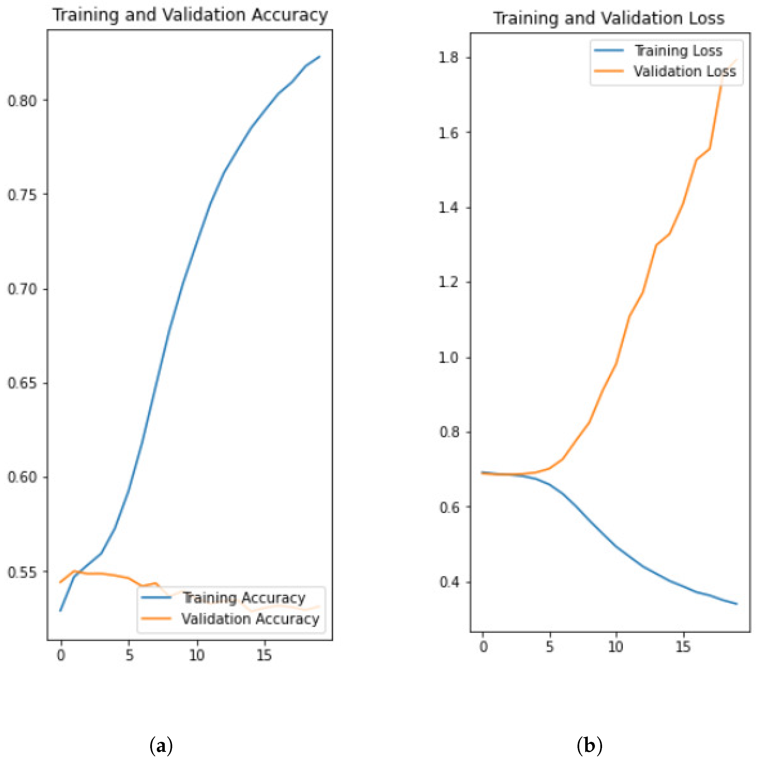
Lastly, even though image and some of the text approaches used in this study were based on the same class of deep neural networks (CNNs), the classification accuracy was significantly low for original avatars in relation to texts (i.e., a decrease from about 62-65% to around 59% in terms of accuracy). Particularly, if we additionally consider that our image classifiers conducted a two-sided task by targeting solely at the two youngest cohorts. As a logical conclusion, it is harder to infer high quality predictors for age from profile pictures than from texts. In reality, we also found it hard to label each individual by an eyeball inspection of his/her profile picture only.

8. Conclusions and Further Work

This work is breaking new ground in cQA research by addressing the key challenges faced by supervised learning when automatically identifying age groups across their community fellows. In particular, it discusses class imbalances, different class distributions across distinct modalities (i.e., texts, images and meta-data) and the gradual evolution from one cluster to the next.

By devising a random forest classifier from the meta-data viewpoint and an age-batched curriculum learner operating on text, we discovered a way of mitigating the effects of class imbalances. In essence, instances close to generational borders must be carefully selected and the distribution of classes must adjust to the diversity of each cohort. In the same vein, putting together all under-represented age cohorts into one cluster proves to be an efficient strategy, when conceiving age prediction as a classification task.

Although our age-batched curriculum learner presents interesting qualitative and quantitative findings on Yahoo! Answers, its application to textual inputs distilled from other sorts of social media networks still remains an open research question, because of the complexity and diversity that are intrinsic to this area of human activity.

As future work, we envisage the extension of this study to consider not only extra techniques for coping with unbalanced data, but also to cover other kinds of views, such as user activity, which would give access to additional, and hopefully highly reliable predictors. In so doing, a battery of graph mining algorithms should be utilized for determining sub-graphs, roles and centralities, just to name a few.

Despite the poor performance reaped by visual classifiers on original avatars, we do not think that the task is desperately lost for them. As a means of enhancing their accuracy, we envision a preliminary step consisting of clustering images into distinct types of profile images (e.g., faces and animals), which which subsequent classifiers will be trained, this way facilitating the task of inferring visual predictive patterns.

Since AGCL is built on top of a greedy search algorithm, it can get trapped in local optima; therefore, the curriculum discovered by the algorithm is highly unlikely to be the optimal, albeit a good one. While it is true that the amount of combinations is small when considering three cohorts, thereby increasing the likelihood of finding the optimal curriculum, it is also true that this number might skyrocket if a larger amount of age groups is considered or if cohorts are modeled with a finer granularity (e.g., per month). Note here also that the level of granularity used by AGCL depends on how well these fine-grained clusters are represented.

All in all, we envisage that our findings will be highly relevant as guidelines for constructing assorted multimodal supervised models for automatic age recognition across cQAs and other sorts of online social networks. In particular, we contemplate as a possibility that our outcomes will aid in the design of multi-view and/or transfer learning models.