Article

Prediction Method of Multiple Related Time Series Based on Generative Adversarial Networks

School of Computer Science and Engineering, Central South University, Changsha 410083, China
*
Author to whom correspondence should be addressed.
Information 2021, 12(2), 55; https://doi.org/10.3390/info12020055
Submission received: 25 December 2020 / Revised: 16 January 2021 / Accepted: 22 January 2021 / Published: 26 January 2021

Abstract

:
In multiple related time series prediction problems, the key is capturing the comprehensive influence of the temporal dependencies within each time series and the interactional dependencies between time series. At present, most time series prediction methods are difficult to capture the complex interaction between time series, which seriously affects the prediction results. In this paper, we propose a novel deep learning model Multiple Time Series Generative Adversarial Networks (MTSGAN) based on generative adversarial networks to solve this problem. MTSGAN is mainly composed of three components: interaction matrix generator, prediction generator, and time series discriminator. In our model, graph convolutional networks are used to extract interactional dependencies, and long short-term memory networks are used to extract temporal dependencies. Through the adversarial training between the generator and the discriminator, we enable the final prediction generator to generate prediction values that are very close to the true values. At last, we compare the prediction performance of the MTSGAN with other benchmarks on different datasets to prove the effectiveness of our proposed model, and we find that MTSGAN model consistently outperforms other state-of-the-art methods in the multiple related time series prediction problems.

1. Introduction

Time series refers to a series of numbers representing the same statistical indicator arranged in the order of their occurrence time. In the real world, time series data is ubiquitous, such as precipitation, electricity consumption, sales of commodities, and stock price. Time series prediction is predicting the future value by mining the implicit pattern in the history values. For a long time, the research on time series prediction problems has attracted a lot of attention of many scholars. In the early stage of studying time series, the autoregressive integrated moving average (ARIMA) [1] model was widely used in time series prediction problems. However, that model is based on the linear regression theory in statistics, and it is essentially a linear model, which has obvious deficiency in fitting data with complex nonlinear patterns. In recent years, with the continuous development of artificial intelligence, many machine learning and deep learning methods have also been used in time series prediction problems, such as support vector machines and neural networks, and these models have the advantage of fitting data with complex nonlinear patterns. So far, most of these studies have focused on single time series prediction problems, and have achieved good results and applications.
However, in the real world, the problems we encounter are often more complex, and the objects we need to study often contain many time series, in which there are time series correlation. The problem of multiple related time series prediction is more complicated than the problem only containing a single time series. We not only need to take into consideration temporal dependencies within each time series but also the interactional dependencies between different time series. How to effectively capture these interactional dependencies is the biggest challenge to solve the multiple related time series prediction problems.
Inspired by the generative adversarial networks, we propose a sequence generation model Multiple Time Series Generative Adversarial Networks (MTSGAN) combined with a graph learning model to solve the prediction problem of multiple related time series. The MTSGAN is designed by using Generative Adversarial Networks [2] (GAN) as the basic model framework and combines the advantages of the Graph Convolutional Networks [3] (GCN) and the Long Short-Term Memory [4] (LSTM). Specifically, there are two alternate stages in the training of MTSGAN. During the generation stage, MTSGAN first maps a random noise vector to an interaction matrix through a generator, which is a symmetric matrix used to represent the interactional dependencies between time series, and then uses GCN to process the complex interactional dependencies, finally using LSTM to separately process the temporal dependencies contained within each time series and generate the prediction values. During the discrimination stage, MTSGAN will train a good discriminator to distinguish between real samples and fake samples generated by generator. Through the adversarial training between generator and discriminator, the generator can finally generate the prediction value very close to the true value.
The main contributions of this paper are summarized below:
(1)
We propose a novel GAN-based deep learning model MTSGAN, which is an end-to-end solution to the prediction problem of multiple related time series that exist widely in the real world. Compared with other existing time series prediction models, MTSGAN can simultaneously capture the complex interactional dependencies between time series and the temporal dependencies within each time series, which has unique advantages in the multiple related time series prediction task.
(2)
In the multiple related time series prediction problem, the complex interactional dependencies between time series is hidden in the data. Conventional methods cannot directly extract these hidden complex interactional dependencies. The MTSGAN model we proposed skillfully uses a generator to generate these interactional dependencies and uses a discriminator to optimize the generated interactional dependencies. This method of directly extracting interactional dependencies from data does not rely on other prior knowledge. In addition, we use transposed convolutional networks to implement our interaction matrix generator, which improves the scalability of MTSGAN.
The rest of the paper is organized as follows. Section 2 introduces the related work. Some definitions of the multiple related time series prediction problem and MTSGAN model details are shown in Section 3. In Section 4, we introduce our experiments results. Section 5 gives the conclusion and future work of this paper.

2. Related Work

2.1. Time Series Prediction

Early time series prediction methods are based on linear regression theory in statistics. In 1970, American statisticians Box and Jenkins first proposed the autoregressive integrated moving average model [1] (ARIMA), which adds a d-order difference process on the basis of the ARIMA model, which can convert non-stationary time series into stationary time series, which extends the method that can only model stationary time series to non-stationary time series. The ARIMA method has greatly promoted the application and development of time series analysis and prediction in various industries and has received widespread attention.
With the development of artificial intelligence, many machine learning methods have been introduced into the field of time series prediction. In 1996, Drucker et al. proposed Support Vector Regression [5] (SVR), which is a regression version of the well-known machine learning method Support Vector Machine [6] (SVM). The solid theoretical foundation of support vector machine ensures that it has unique advantages in solving small samples, high-dimensional data and nonlinear problems. Kim [7] directly used support vector machines to predict the stock price index. Tay and Cao [8] directly used support vector machine to predict financial time series data and tested the feasibility of the method through comparative experiments. Hao et al. [9] used SVR with a modified regular function to predict the stock composite index and achieved good results. In addition to applying SVM to financial time series prediction, Mellit et al. [10] also used SVM to predict meteorological time series data.
Deep learning is a subfield of machine learning. LSTM and its variant Gate Recurrent Unit (GRU) are deep learning models, which are widely used to process sequential data. They are also being used to predict time series. LSTM can solve the multiple related time series prediction problem by feeding multiple time series in parallel. The proposed model still has three advantages over LSTM: (1) LSTM relies on the cell state that is a vector to memorize the information of dependency in the input sequential data. If we want to simultaneously capture the temporal dependencies within the time series and the interactional dependencies between the time series through LSTM, we need LSTM to compress the input matrix into a vector, in which each column represents a time series. This will definitely lose some information. However, in MTSGAN, the dependency information of two aspects will be stored in an intermediate feature representation, which is the same size as the input matrix. This ensures that the information will not be lost. (2) MTSGAN uses an interaction matrix generator to generate the interaction dependencies between time series, and then can explicitly model the dependencies on the graph by capturing more complex adjacency dependencies, including first-order adjacency dependencies between node and its neighbor, second-order adjacency dependencies between node and neighbor of its neighbor, and so on. But LSTM models the dependencies in an implicit way, which can only capture first-order adjacency dependencies as far as possible.
Multivariate time series prediction is very similar to our research work. A multivariate time series contains more than one time-dependent variable, and each variable not only depends on its past historical values but also on other variables. The vector autoregressive model [11] (VAR) is one of the most commonly used methods to solve the multivariate time series forecasting problem. The dimension of the multivariate time series processed by this method is usually low, and the dependencies between different variables is not very complicated. However, multiple related time series prediction usually contains a large number of time series, and there are often complex interactional dependencies between time series. In the VAR model, the predicted value of each variable is obtained by linear regression of the historical values of the variable and the historical values of other variables. Although VAR can take into account the dependencies between different variables, it is still a linear model in nature. It is limited by model assumptions when fitting data with complex nonlinear pattern, so it is difficult to obtain satisfactory prediction results.
Another problem very similar to our research work is traffic prediction. The research objects in traffic prediction are spatial-temporal sequences. Usually, the traffic volume data recorded by sensors on each road segment over time can form a time series. These time series have different adjacency relations geographically, and these adjacency relations are usually regarded as dependencies between time series. Reference [12] proposed a multi-graph convolutional network to predict shared bike flow, and Reference [13] combined graph convolutional neural network and gated recurrent unit to propose a new model T-GCN to solve the traffic prediction problem. Our research work is different from the traffic prediction problem. The dependencies between time series in traffic prediction are determined by the geographical position relations between time series, which depends on prior knowledge. But the interactional dependencies between time series in our studying problem are implicit and exist in the data. We use a generative method to mine these interactional dependencies from the data with the help of MTSGAN and apply it to multiple time series prediction problems.

2.2. GAN and GCN

Generative Adversarial Networks [2] (GAN) was proposed by Goodfellow in 2014. Specifically, a GAN mainly contains two neural networks: a generator and a discriminator. The task of the generator is to map the random noise vector to synthetic data; the discriminator takes real data and synthetic data as input, and outputs the probability that this sample is true. At present, GAN is mainly used in the field of computer vision and is used to generate realistic synthetic images. There is almost no research on applying GAN to multiple time series prediction problems. The only relevant one is the use of GAN in Reference [14] to deal with missing values in multivariate time series. As far as we know, our research work should be the first to apply GAN to multiple related time series prediction problem.
The graph convolutional network is a brand new neural network model recently proposed. It is different from the traditional neural network that can only process euclidean structure data. The object processed by the graph convolutional network is the graph structure data. The graph convolutional network was first proposed by Bruna et al. [15] in 2013, and then Defferrard et al. [16] further improved the graph convolution by reducing the complexity of the calculation process by designing a fast localized spectral convolution kernel on the graph. Kipf et al. [3] designed the widely used graph convolutional network by doing a first order local approximation of the spectral convolution and achieved good results in the task of semi-supervised classification of literature cited data. The graph convolutional network in the following description refers to the graph convolutional network (GCN) proposed by Kipf et al., unless otherwise specified. GCN has attracted great interest of researchers, and they have begun to use GCN to solve complex problems in various fields. For example, Reference [17] uses GCN to classify text, and Reference [18] uses GCN to predict diseases.

3. Proposed Model

3.1. Problem Definition

Multiple related time series prediction problem: suppose that the object we are studying contains n time series T 1 , T 2 , , T n ; the time step we need to predict is t + 1 , so the data features we can get are T 1 [ t w + 1 , t ] , T 2 [ t w + 1 , t ] , , T n [ t w + 1 , t ] , which represents the historical values of each series in a sliding window of length w. Our goal is to train a model f to map the above data features to the future values of each time series at time step t + 1 :
[ T 1 t + 1 , , T n t + 1 ] = f ( T 1 [ t w + 1 , t ] , , T n [ t w + 1 , t ] ) .
Definition 1.
Time series feature vector T i [ t w + 1 , t ] . The time series feature vector is a feature vector composed of historical values covered by a sliding window of length w at the time step t. The i-th time series feature vector representation is as follows:
T i [ t w + 1 , t ] = [ T i t w + 1 , T i t w + 2 , , T i t ] .
Definition 2.
Time series feature matrix X n × w . The time series feature matrix is composed of n time series feature vectors, and each row in the matrix corresponds to a time series feature vector. The number of columns in the matrix is equal to the length of the sliding window w, and the number of rows in the matrix is equal to the number of time series n. The representation of time series feature matrix is as follows:
X n × w = T 1 t w + 1 T 1 t w + 2 T 1 t T 2 t w + 1 T 2 t w + 2 T 2 t T n t w + 1 T n t w + 2 T n t .
Definition 3.
Time series interaction graph G. Figure 1 shows a time series interaction graph containing five time series. The interactional dependencies of multiple time series are represented as a weighted undirected graph G = ( V , E ) . V is the set of nodes, each node corresponds to a time series feature vector, and the time series feature matrix X n × w can be used to describe the node set V. The set of weighted edges E represents the weighted adjacency relations between the nodes of the time series interaction graph, which is used to describe the interactional dependencies between time series. The adjacency matrix of the time series interaction graph is represented by A n × n ; we also call it the interaction matrix which is generated by interaction matrix generator; each matrix element corresponds to an edge in E, and the range of its values defined as follows:
A i , j = a , ( i j a n d 0 a 1 ) 0 , ( i = j ) .

3.2. MTSGAN Overview
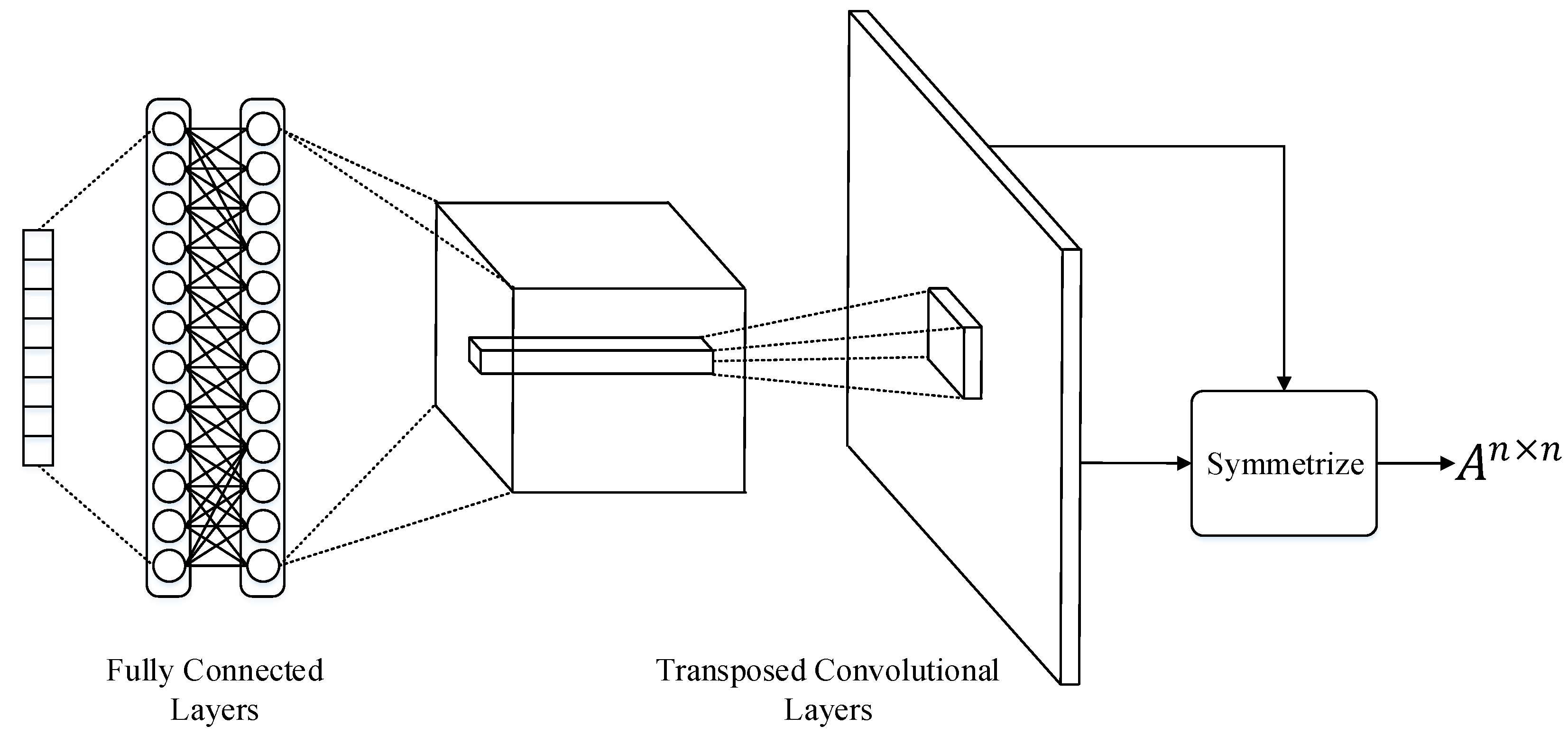
The original GAN was proposed in Reference [2]. GAN contains two networks. One is the generation network, and the other is the discrimination network. GAN makes the samples generated by the generation network obey the real data distribution through adversarial training between two networks. MTSGAN is a deep learning model based on GAN. The overall architecture of the model is shown in Figure 2. Similar to the structure of the classic generative adversarial networks, MTSGAN is composed of an interaction matrix generator G i , a prediction generator G p , and a time series discriminator D. The specific descriptions of these three components are as follows:
  • Interaction Matrix Generator G i : G i consists of a transposed convolutional networks, which implements a mapping function f : R k R n × n . It maps a k dimensional random noise vector sampled from the Gaussian distribution to a n × n interaction matrix. We use this interaction matrix as the adjacency matrix of the time series interaction graph.
  • Prediction Generator G p : G p consists of a graph convolutional networks (GCN) and a long short-term memory networks (LSTM). Its input is a time series interaction graph, which is described by an interaction matrix and a time series feature matrix. First, GCN performs graph convolution operations on the time series interaction graph to obtain an intermediate feature representation that incorporates the interactional dependencies between time series, and then LSTM processes this intermediate feature representation and capture the temporal dependencies. In this way, the predicted value of each time series can be generated by the prediction generator.
  • Time Series Discriminator D: The discriminator is used to judge the quality of the data generated by the prediction generator. It takes real time series samples and fake time series samples as input, and then outputs a value indicating the probability that the input sample is true. After the discriminator is well trained, it will be fixed as an estimator of the above two generators, and the gradient information will be fed back to G i and G p to optimize its parameters.
The overall workflow of MTSGAN can be divided into a generation process, a discrimination process and an adversarial process. In the generation process, first, the interaction matrix generator transforms a random noise vector into an interaction matrix and then combines the interaction matrix with the time series feature matrix to construct a time series interaction graph. Next, the prediction generator capturea the interactional dependencies between time series and temporal dependencies within each time series to generate the predicted value of each time series. In the discrimination process, first, it is necessary to construct real samples and fake samples. We use the real data represented by the time series feature matrix and real targets to obtain real time series samples through matrix concatenating operation, as well as use the real data and fake targets generated by the prediction generator to obtain fake time series samples through matrix concatenating operation. Then, the discriminator will use real samples and fake samples as the training set for training. When it can correctly distinguish between real samples and fake samples, the discriminator training is completed. In the adversarial process, the well trained discriminator is fixed as the generators’ evaluator, and the network parameters of two generators are adjusted to maximize the probability that the fake samples generated by the two generators are judged to be real samples by the discriminator.
The process of G i , G p , and D as the two parties’ competitors playing the minimax game can be formally expressed as Equation (5), which is derived from GAN [2]. Finally, the overall logic of MTSGAN is summarized in Algorithm 1.
min θ i , θ p max θ d V ( G i , G p , D ) = min θ i , θ p max θ d E y p t r u e ( · | x ) [ log D ( y , X ; θ d ] + E z p ( z ) [ log ( 1 D ( G p ( G i ( z ; θ i ) , X ; θ p ) , X ; θ d ) ) ] .
Algorithm 1 MTSGAN Framework
Input: time series feature vector { T 1 [ t w + 1 , t ] , T 2 [ t w + 1 , t ] , , T n [ t w + 1 , t ] } , real target { T 1 t + 1 , T 2 t + 1 , , T n t + 1 }
Output: prediction values { T 1 ^ t + 1 , T 2 ^ t + 1 , , T n ^ t + 1 } , generator G i , G p and discriminator D
 1: Initialize G i ( ; θ i ) , G p ( ; θ p ) , D ( ; θ d )
 2: for number of training iterations do
 3:     generate the random noise z N ( 0 , 1 )
 4:     generate the interaction matrix A ^ = G i ( z ; θ i )
 5:     make interaction matrix symmetrical:              A ^ = ( A ^ + A ^ T ) / 2    and     A ^ i i = 0
 6:     construct time series feature matrix:
X = T 1 t w + 1 T 1 t w + 2 T 1 t T 2 t w + 1 T 2 t w + 2 T 2 t T n t w + 1 T n t w + 2 T n t

 7:     generate the prediction values { T 1 ^ t + 1 , T 2 ^ t + 1 , , T n ^ t + 1 } = G p ( A ^ , X ; θ p )
 8:     construct real time series samples:              T i [ t w + 1 , t + 1 ] = [ T i t w + 1 , T i t w + 2 , , T i t , T i t + 1 ]
 9:     construct fake time series samples:              T i ^ [ t w + 1 , t + 1 ] = [ T i t w + 1 , T i t w + 2 , , T i t , T i ^ t + 1 ]
10:     for k steps do
11:         training D ( ; θ d ) to distinguish real samples from fake samples
12:         update discriminator by ascending its gradient:              θ d θ d + α · θ d V ( G i , G p , D )
13:     end for
14:     generate the random noise z N ( 0 , 1 )
15:     update the G i ( ; θ i ) by descending its gradient:              θ i θ i α · θ i V ( G i , G p , D )
16:     update the G p ( ; θ p ) by descending its gradient:              θ p θ p α · θ p V ( G i , G p , D )
17: end for
18: generate the random noise z N ( 0 , 1 )
19: get prediction values { T 1 ^ t + 1 , T 2 ^ t + 1 , , T n ^ t + 1 } = G p ( G i ( z ; θ i ) , X ; θ p )
20: return { T 1 ^ t + 1 , T 2 ^ t + 1 , , T n ^ t + 1 } , G i , G p , D

3.3. Interaction Matrix Generator

The role of the interaction matrix generator is to generate a matrix. If we regard the matrix as a picture, the role of the interaction matrix generator is similar to that of the generator in DCGAN [19], so we use transposed convolution [20] to implement the interaction matrix generator. The effects of transposed convolution and convolution are exactly opposite. The convolution operation can transform a fine-grained representation into a coarse-grained representation, which is equivalent to a down-sampling method; while transposed convolution operation can transform a coarse-grained representation into a fine-grained representation, which is equivalent to an up-sampling method. The transposed convolutional network has the advantages of local connectivity and kernel parameter sharing. Compared with fully connected networks, it can greatly reduce the number of network parameters and is more efficient when processing large scale data. The structure of the interaction matrix generator we implemented is shown in Figure 3. A high dimensional random noise vector sampled from the Gaussian distribution will be used as the input of the interaction matrix generator. The noise vector is mapped to a three-dimensional feature map through a fully connected layer, the three dimensions are length, width, and number of channels. The transposed convolutional layers will continue to process the three-dimensional feature map. Each time through a transposed convolutional layer, the number of channels of the feature map will decrease, the length and the width will increase. Finally, the output of the transposed convolutional layers is a tensor in which dimension is n × n × 1 , where n is the number of time series we need to process. The output result of the transposed convolutional layers cannot be used directly as an interaction matrix, and it needs to be symmetric. The symmetrization operation is shown in Equation (6), where O is the output matrix of the transposed convolutional layers, and A is the symmetric matrix obtained after processing.
A i , j = ( O i , j + O j , i ) / 2 , ( i j ) 0 , ( i = j ) .

3.4. Prediction Generator

It has been explained before that in multiple related time series prediction problems, there are two dependencies that need to be dealt with: (1) interactional dependencies between the time series; and (2) temporal dependencies within each time series. The interactional dependencies has been obtained through an interaction matrix generator. Our purpose of designing a prediction generator is to comprehensively deal with these two kinds of dependencies. Our prediction generator is shown in Figure 4. We use the interaction matrix as the adjacency matrix and the time series feature matrix as the feature matrix of the graph to construct a time series interaction graph. The time series feature vector on each node in the graph contains the temporal dependencies within each time series, and the weighted edges between nodes contain the interactional dependencies between the time series. As a well-known graph representation learning algorithm, GCN has the advantage of efficiently processing graph structured data. Using GCN to process time series interaction graphs can get an intermediate feature representation. Specifically, in Figure 1, node set {1, 2, 4} is the input of the graph convolution on node 1, in which node 1 is the central node, and node 2 and node 4 are the neighbor nodes of node 1. So, the output of graph convolution is the weight sum of central node feature and its neighbor node feature. The same is true for the node set {2, 1, 4} and node set {6, 3, 4, 5}. From the perspective of graph embedding, GCN embeds the topological information in the time series interaction graph, that is, the information in the edges into the output intermediate feature representation. So, the intermediate feature representation we get actually contains two aspects of information: (1) the information in the time series feature matrix containing the temporal dependencies within each time series; and (2) the information in the interaction matrix containing the interactional dependencies between time series. Finally, we use LSTM [4] to process this intermediate feature representation and generate the final predicted values.

3.4.1. GCN for Extracting Interactional Dependencies

GCN is used to model the interactional dependencies between time series. The graph convolutional layer in MTSGAN is shown in Equation (7):
H = GCN ( A , X ) = f ( D ˜ 1 2 A ˜ D ˜ 1 2 X W ) ,
where A ˜ = A + I , A is the interaction matrix generated by the generator, and I is the identity matrix. Converting A to A ˜ is equivalent to adding a self loop edge for each node. The purpose of that is to prevent losing original information of the node itself during the operation of graph convolution. Matrix D ˜ is the degree matrix corresponding to A ˜ . The elements on the main diagonal are D ˜ i i = j = 1 n A ˜ i j , and the other elements are 0. A ˜ left multiplied by D ˜ 1 2 and right multiplied by D ˜ 1 2 is the normalization process to prevent the problem of inconsistent scales of node features in graph convolution operation. X R n × w is the time series feature matrix on the graph, each row of the matrix is a time series feature vector, and W R w × w is the learnable parameter in GCN. H R n × w is the representation matrix obtained after graph convolution.

3.4.2. LSTM for Extracting Temporal Dependencies

LSTM uses some gate structure to allow information to selectively affect the state of each moment in the recurrent neural network. The so-called gate structure is a mini neural network using a sigmoid activation function and a element-wise multiplication operation. It is called the gate structure because the fully connected neural network layer using sigmoid as the activation function will output a value between 0 and 1, describing how much information the current output can pass through this gate structure. When the door is fully opened, that is, when the sigmoid output is 1, all information can pass; when the door is completely closed, that is, the sigmoid output is 0, all information cannot be passed. The following is the definition of each gate in LSTM:
z = tanh ( W z [ h t 1 , x t ] + b z ) ,
i = s i g m o i d ( W i [ h t 1 , x t ] + b i ) ,
f = s i g m o i d ( W f [ h t 1 , x t ] + b f ) ,
o = s i g m o i d ( W o [ h t 1 , x t ] + b o ) ,
c t = f c t 1 + i z ,
h t = o tanh ( c t ) ,
where i, f, and o represent input gate, forget gate, and output gate, respectively, and c t represents the memory unit at time t, which can be regarded as a representation vector of the previous input sequence information. h t represents the output value at time t. W and b, respectively, represent the weight parameter and bias parameter corresponding to each gate in LSTM.

3.5. Time Series Discriminator

In the original GAN, the discriminator, as an opponent in the minimax game with the generator, needs to make a correct distinction between the data generated by the generator and the real data. In the MTSGAN model, the prediction generator generates the prediction value of each time series. In our problem, it is not meaningful to directly use the scheme in GAN to let the discriminator distinguish between the predicted value and the true value, or this method is not applicable to the problem we are studying. Our improved method is to add the generated prediction value to the original time series feature vector to construct a fake time series sample, as well as to add the true value to the original time series feature vector to construct a real time series sample. Equations (14) and (15), respectively, represent the specific forms of fake time series samples and real time series samples.
T i ^ [ t w + 1 , t + 1 ] = [ T i t w + 1 , T i t w + 2 , , T i t , T i ^ t + 1 ] ,
T i [ t w + 1 , t + 1 ] = [ T i t w + 1 , T i t w + 2 , , T i t , T i t + 1 ] .
The role of the time series discriminator is to correctly distinguish the true and fake time series samples constructed above, for which implementation details are shown in Figure 5. The entire discriminator contains two input terminals. One of the inputs is the embedding layers, which takes a one-hot encoding vector as input, and outputs a low dimensional dense vector. The one-hot encoding vector is a sparse vector with a very high dimension, used to distinguish which time series in the dataset the current time series sample comes from. The other input terminal is a bidirectional long short-term memory network [21], which takes a time series sample as input. The main structure of the bidirectional long short-term memory network is the combination of two unidirectional LSTMs. At each time t, the input will be provided to the two LSTMs in opposite directions. The two LSTMs are calculated independently, and each generates the hidden state and output at that moment. The two unidirectional LSTMs are symmetrical except for the different directions. The output of FLSTM at the last time step encodes the forward temporal information in the time series sample, and the output of BLSTM at the first time step encodes the reverse temporal information of the time series sample. The output of the bidirectional long short-term memory networks is actually the concatenation of FLSTM’s output vector and BLSTM’s output vector. Finally, in our time series discriminator, the vector output by the embedding layer and the vector output by the bidirectional long short-term memory network will be concatenated together and input into a fully connected network, in which output value is the probability that the input time series sample is true.

4. Experiments

In order to verify the effectiveness of the MTSGAN model, we compared the prediction performance of the MTSGAN model and other state-of-art methods on different datasets, and used different metrics for evaluation. Then, we experimentally studied the influence of the model structure on the performance of MTSGAN, that is, the influence of the interaction matrix generator structure and the depth of the GCN network on the prediction performance.

4.1. Data Sets

  • Store Item Demand Dataset (https://www.kaggle.com/c/demand-forecasting-kernels-only/data). This dataset provides daily sale records of 50 different products in 10 different stores. The sale records of each product start on 1 January 2013 and end on 31 December 2017, which means this dataset contains 500 time series, and the length of each time series is 1826 days.
  • Web Traffic Dataset (https://www.kaggle.com/c/web-traffic-time-series-forecasting/data). This dataset records the data of Wikipedia website traffic. The entire dataset contains about 145,000 time series. Each time series represents the daily traffic of a Wikipedia page. The recording time starts from 1 July 2015 to 10 September 2017. The length of time series is 804 days. The dataset contains missing values, and the data used in the experiment is 500 time series that do not contain missing values.
  • NOAA China Dataset (https://www.ncei.noaa.gov/data/global-summary-of-the-day/). This dataset is the meteorological data recorded by weather stations in different locations in China provided by the National Oceanic and Atmospheric Administration of the United States. We extracted daily temperature data from 400 different weather stations from 2015 to 2018 as our experimental data.

4.2. Experimental Settings

We use the Pytorch (https://pytorch.org/) deep learning framework to implement MTSGAN. In the interaction matrix generator, the dimension of the random noise vector is set to 512, and it is sampled from a Gaussian distribution. In the prediction generator, the number of GCN layers is set to 3, the number of hidden layers of LSTM is set to 3, and the dimension of the hidden layer is set to 64. Since the LSTM finally needs to generate a scalar value, the output of the LSTM needs to go through a fully connected layer to transform the dimension from 64 to 1. In the time series discriminator, the dimension of the embedding layer vector is set to 8, the number of hidden layers of the bidirectional long short-term memory networks is set to 3, and the dimension of the hidden layer is set to 64. In the process of training model, the learning rate is set to 0.001, the batch size parameter is set to 16, Adam [22] is used as the optimization algorithm, and the Dropout [23,24] technique is used to avoid overfitting of the model, for which parameter is set to 0.2.
The prediction performance of the MTSGAN model will be compared with the following methods:
(1)
Autogressive Integrated Moving Average [1] (ARIMA): This method first make the time series stationary through a difference operation, and then combines the AR model and the MA model to predict the future value of the time series. It is a very widely used time series prediction method.
(2)
Vector Auto-Regressive [11] (VAR): This model is often used to solve the prediction problem of multivariate time series. It can consider the correlation between variables of different dimensions.
(3)
Support Vector Regression machines [5] (SVR): This model is a well-known machine learning model with solid mathematical theoretical support.
(4)
LightGBM [25] (LGB): This model is an improved gradient boosting tree model, which can solve classification and regression problems, and demonstrates powerful prediction performance in various data mining competitions.
(5)
Long Short-Term Memory [4] (LSTM): This model is a recurrent neural network model that can capture long-distance dependencies in sequence data.
(6)
Gate Recurrent Unit [26] (GRU): This model is also a recurrent neural network model, which simplifies the gate structure in LSTM and makes training more efficient.

4.3. Prediction Performance of MTSGAN

Table 1 shows the prediction performance comparison of MTSGAN and other six methods on the three datasets of Store Item, Web Traffic, and NOAA China. In the six methods of comparison, ARIMA and VAR are statistical methods; SVR and LGB are machine learning methods; LSTM and GRU are deep learning methods. From the table, we can see that under the two evaluation metrics of MAE and RMSE, the model we proposed has the best prediction results on the three datasets. Among other comparison methods, ARIMA is a single time series prediction method. In the multiple related time series prediction problem we studied, this method did not take into account the interactional dependencies between the time series, in which prediction results in the experiment is the worst. In the experiment, VAR model converts multiple related time series prediction problem into a multivariate time series prediction problem. This method can capture the correlation between time series to a certain extent. However, because it is a linear model, in which ability to fit data with complex patterns is limited, its prediction results are only better than the ARIMA model. Both SVR and LGB are excellent machine learning models, and their prediction results are very close. LGB is slightly better than SVR overall. Both LSTM and GRU are deep learning models and are very similar in structure. The prediction results of LSTM is slightly better than that of GRU, but, from the perspective of model training, the training efficiency of GRU is significantly better than that of LSTM. Comparing with LGB and LSTM, the former has better results on the Store Item and NOAA China datasets, and the latter has better results on the Web Traffic dataset. Based on the results of the entire experiment, the prediction results of MTSGAN on the three dataset completely outperform the other six methods, which proves that our proposed model has obvious advantages in the multiple related time series prediction problem.

4.4. Influence of Interaction Matrix Generator’s Structure

We conducted a comparative experiment on the influence of using fully connected networks and transposed convolutional networks to implement the interaction matrix generator on the prediction performance of the MTSGAN model. The results of the experiment are shown in Figure 6. The figure in each row represents the prediction result on a certain evaluation metric, and the figure in each column represents the prediction result on a certain dataset. The “FCN” in the figure represents the fully connected networks, and “Tconv” represents a transposed convolutional networks. In each subfigure, the specific meaning of the independent variable on the horizontal axis is the number of time series in the dataset used by the model; the specific meaning of the dependent variable on the vertical axis is the prediction result of the model under a certain metric. Through our experiments, we found that when the number of time series is small, for example, between 50 and 100, there is little difference in the prediction performance of two network structures. However, with the gradual increase in the number of time series, the prediction performance of the model implemented by the transposed convolutional networks is better than that of the fully connected networks, and the greater the number of time series, the more obvious the difference. This advantage of the transposed convolutional network may be because it has the characteristics of local connectivity and parameter sharing similar to the convolutional network, so the transposed convolutional network is more efficient in processing two-dimensional grid data, and it is used to implement MTSGAN with better prediction performance.

4.5. Influence of GCN Depth

In this experiment, we studied the influence of the number of GCN layers on the prediction performance of the MTSGAN. The specific experimental results are shown in Figure 7. We measure the different prediction performance of the model on the training set and the test set under the conditions of different GCN layers on three datasets. The evaluation metric of the prediction results in the first row of figures is MAE, and the second row of figures is RMSE. We found that under these two evaluation metrics, when the number of GCN layers is 3 or 4, the model has the best fitting ability (the training set has the smallest error) and the best generalization ability (the test set has the smallest error). When the number of GCN layers is less than 3, the model does not fully fit the data. At this time, the training error and generalization error will gradually decrease as the number of GCN layers increases. When the number of GCN layers exceeds 6, the model begins to overfit. At this time, the generalization error increases significantly as the number of GCN layers increases.

5. Conclusions

This paper proposes a novel deep learning model MTSGAN for multiple related time series prediction problems. The model is based on the architecture of a generative adversarial network, which consists of two generators and one discriminator. The discriminator helps the two generators to optimize their own parameters by means of adversarial training and finally makes the generated data very close to the true data. In the experiment, we first compared the prediction performance of MTSGAN and other six methods on three datasets. The results of the experiment show that the prediction performance of MTSGAN completely outperform other methods. In addition, we conducted two experiments on the impact of the model structure on the prediction performance of MTSGAN. These experiments can guide us to better use MTSGAN in applications to solve practical problems.
MTSGAN is a novel end-to-end solution to multiple related time series prediction problem that exists widely in the real word. Based on MTSGAN model framework to develop a prediction system to solve the relevant problems in the industry is our future work. A common industrial scenario of applying the prediction system is predicting sales of many commodities to help shop owner arrange inventory reasonably to increase revenue and reduce costs. Our following work will take more additional features into consideration, such as holiday information, weather information, and further expand the model to enable it to perform multi-step predictions of time series.

Author Contributions

Conceptualization, W.W. and F.H.; methodology, W.W. and F.H.; software, W.W.; validation, W.W., Y.K., Z.C. and Q.W.; formal analysis, W.W. and F.H.; investigation, W.W.; data curation, Y.K., Z.C. and Q.W.; writing—original draft preparation, W.W.; writing—review and editing, W.W., F.H., Y.K., Z.C. and Q.W.; visualization, W.W.; supervision, F.H.; project administration, F.H.; funding acquisition, F.H. All authors have read and agreed to the published version of the manuscript.

Funding

This research was funded by Science and Technology Plan of Hunan Province Project grant number 2016JC2011.

Institutional Review Board Statement

Not applicable.

Informed Consent Statement

Not applicable.

Data Availability Statement

Data is contained within the article.

Conflicts of Interest

The authors declare no conflict of interest.

References

  1. Box, G.E.P.; Jenkins, G. Time Series Analysis, Forecasting and Control; Holden-Day, Inc.: Stoakland, CA, USA, 1990. [Google Scholar]
  2. Goodfellow, I.; Pouget-Abadie, J.; Mirza, M.; Xu, B.; Warde-Farley, D.; Ozair, S.; Courville, A.; Bengio, Y. Generative adversarial nets. Adv. Neural Inf. Process. Syst. 2014, 27, 2672–2680. [Google Scholar]
  3. Kipf, T.N.; Welling, M. Semi-supervised classification with graph convolutional networks. arXiv 2016, arXiv:1609.02907. [Google Scholar]
  4. Hochreiter, S.; Schmidhuber, J. Long short-term memory. Neural Comput. 1997, 9, 1735–1780. [Google Scholar] [CrossRef] [PubMed]
  5. Drucker, H.; Burges, C.J.; Kaufman, L.; Smola, A.; Vapnik, V. Support vector regression machines. Adv. Neural Inf. Process. Syst. 1996, 9, 155–161. [Google Scholar]
  6. Cortes, C.; Vapnik, V. Support-vector networks. Mach. Learn. 1995, 20, 273–297. [Google Scholar] [CrossRef]
  7. Kim, K.J. Financial time series forecasting using support vector machines. Neurocomputing 2003, 55, 307–319. [Google Scholar] [CrossRef]
  8. Tay, F.E.; Cao, L. Application of support vector machines in financial time series forecasting. Omega 2001, 29, 309–317. [Google Scholar] [CrossRef]
  9. Hao, W.; Yu, S. Support vector regression for financial time series forecasting. In International Conference on Programming Languages for Manufacturing; Springer: Boston, MA, USA, 2006; pp. 825–830. [Google Scholar]
  10. Mellit, A.; Pavan, A.M.; Benghanem, M. Least squares support vector machine for short-term prediction of meteorological time series. Theor. Appl. Climatol. 2013, 111, 297–307. [Google Scholar] [CrossRef]
  11. Zivot, E.; Wang, J. Vector autoregressive models for multivariate time series. In Modeling Financial Time Series with S-PLUS®; Springer: New York, NY, USA, 2006; pp. 385–429. [Google Scholar]
  12. Chai, D.; Wang, L.; Yang, Q. Bike flow prediction with multi-graph convolutional networks. In Proceedings of the 26th ACM SIGSPATIAL International Conference on Advances in Geographic Information Systems, Seattle, WA, USA, 6–9 November 2018; pp. 397–400. [Google Scholar]
  13. Zhao, L.; Song, Y.; Zhang, C.; Liu, Y.; Wang, P.; Lin, T.; Deng, M.; Li, H. T-gcn: A temporal graph convolutional network for traffic prediction. IEEE Trans. Intell. Transp. Syste. 2019, 21, 3848–3858. [Google Scholar] [CrossRef] [Green Version]
  14. Luo, Y.; Cai, X.; Zhang, Y.; Xu, J. Multivariate Time Series Imputation with Generative Adversarial Networks. Advances in Neural Information Processing Systems. 2018, pp. 1596–1607. Available online: https://papers.nips.cc/paper/7432-multivariate-time-series-imputation-with-generative-adversarial-networks (accessed on 25 January 2021).
  15. Bruna, J.; Zaremba, W.; Szlam, A.; LeCun, Y. Spectral networks and locally connected networks on graphs. arXiv 2013, arXiv:1312.6203. [Google Scholar]
  16. Defferrard, M.; Bresson, X.; Vandergheynst, P. Convolutional neural networks on graphs with fast localized spectral filtering. Adv. Neural Inf. Process. Syst. 2016, 29, 3844–3852. [Google Scholar]
  17. Yao, L.; Mao, C.; Luo, Y. Graph convolutional networks for text classification. In Proceedings of the AAAI Conference on Artificial Intelligence, Honolulu, HI, USA, 5 September 2019; Volume 33, pp. 7370–7377. [Google Scholar]
  18. Parisot, S.; Ktena, S.I.; Ferrante, E.; Lee, M.; Guerrero, R.; Glocker, B.; Rueckert, D. Disease prediction using graph convolutional networks: Application to Autism Spectrum Disorder and Alzheimer’s disease. Med. Image Anal. 2018, 48, 117–130. [Google Scholar] [CrossRef] [PubMed] [Green Version]
  19. Radford, A.; Metz, L.; Chintala, S. Unsupervised representation learning with deep convolutional generative adversarial networks. arXiv 2015, arXiv:1511.06434. [Google Scholar]
  20. Dumoulin, V.; Visin, F. A guide to convolution arithmetic for deep learning. arXiv 2016, arXiv:1603.07285. [Google Scholar]
  21. Schuster, M.; Paliwal, K.K. Bidirectional recurrent neural networks. IEEE Trans. Signal Process. 1997, 45, 2673–2681. [Google Scholar] [CrossRef] [Green Version]
  22. Kingma, D.P.; Ba, J. Adam: A method for stochastic optimization. arXiv 2014, arXiv:1412.6980. [Google Scholar]
  23. Hinton, G.E.; Srivastava, N.; Krizhevsky, A.; Sutskever, I.; Salakhutdinov, R.R. Improving neural networks by preventing co-adaptation of feature detectors. arXiv 2012, arXiv:1207.0580. [Google Scholar]
  24. Srivastava, N.; Hinton, G.; Krizhevsky, A.; Sutskever, I.; Salakhutdinov, R. Dropout: A simple way to prevent neural networks from overfitting. J. Mach. Learn. Res. 2014, 15, 1929–1958. [Google Scholar]
  25. Ke, G.; Meng, Q.; Finley, T.; Wang, T.; Chen, W.; Ma, W.; Ye, Q.; Liu, T.Y. Lightgbm: A highly efficient gradient boosting decision tree. Adv. Neural Inf. Process. Syst. 2017, 30, 3146–3154. [Google Scholar]
  26. Cho, K.; Van Merriënboer, B.; Gulcehre, C.; Bahdanau, D.; Bougares, F.; Schwenk, H.; Bengio, Y. Learning phrase representations using RNN encoder-decoder for statistical machine translation. arXiv 2014, arXiv:1406.1078. [Google Scholar]
Figure 1. Time series interaction graph with five time series.
Information 12 00055 g001
Figure 2. The architecture of the Multiple Time Series Generative Adversarial Network (MTSGAN).
Information 12 00055 g002
Figure 3. Implementation details of the interaction matrix generator.
Information 12 00055 g003
Figure 4. Implementation details of the prediction generator.
Information 12 00055 g004
Figure 5. Implementation details of the time series discriminator.
Information 12 00055 g005
Figure 6. The influence of interaction matrix generator structure on prediction performance.
Information 12 00055 g006
Figure 7. The influence of Graph Convolutional Network (GCN) depth on prediction performance.
Information 12 00055 g007
Table 1. The prediction results of the MTSGAN and other methods.
Store ItemWeb TrafficNOAA China
MAERMSEMAERMSEMAERMSE
ARIMA12.63715.47920.19635.7128.95411.231
VAR7.7149.72916.10831.1977.8069.879
SVR8.41911.52713.48222.7545.6927.539
LGB6.8979.02913.07821.5314.4195.853
LSTM9.11312.21712.31418.5384.7556.436
GRU9.23713.35113.19718.0174.8926.785
MTSGAN5.8437.67510.61016.9683.4674.726
Publisher’s Note: MDPI stays neutral with regard to jurisdictional claims in published maps and institutional affiliations.

