Article

Adaptive Machine Learning for Robust Diagnostics and Control of Time-Varying Particle Accelerator Components and Beams

by
Alexander Scheinker
Los Alamos National Laboratory, Los Alamos, NM 87545, USA
Information 2021, 12(4), 161; https://doi.org/10.3390/info12040161
Submission received: 10 March 2021 / Revised: 27 March 2021 / Accepted: 8 April 2021 / Published: 10 April 2021
(This article belongs to the Special Issue Machine Learning and Accelerator Technology)

Abstract

:
Machine learning (ML) is growing in popularity for various particle accelerator applications including anomaly detection such as faulty beam position monitor or RF fault identification, for non-invasive diagnostics, and for creating surrogate models. ML methods such as neural networks (NN) are useful because they can learn input-output relationships in large complex systems based on large data sets. Once they are trained, methods such as NNs give instant predictions of complex phenomenon, which makes their use as surrogate models especially appealing for speeding up large parameter space searches which otherwise require computationally expensive simulations. However, quickly time varying systems are challenging for ML-based approaches because the actual system dynamics quickly drifts away from the description provided by any fixed data set, degrading the predictive power of any ML method, and limits their applicability for real time feedback control of quickly time-varying accelerator components and beams. In contrast to ML methods, adaptive model-independent feedback algorithms are by design robust to un-modeled changes and disturbances in dynamic systems, but are usually local in nature and susceptible to local extrema. In this work, we propose that the combination of adaptive feedback and machine learning, adaptive machine learning (AML), is a way to combine the global feature learning power of ML methods such as deep neural networks with the robustness of model-independent control. We present an overview of several ML and adaptive control methods, their strengths and limitations, and an overview of AML approaches.

1. Introduction

A simple code for the adaptive control algorithm used here can be downloaded from: https://github.com/alexscheinker/ES_adaptive_optimization, accessed on 8 April 2021. Machine learning (ML) [1] tools such as neural networks (NN) [2], Gaussian processes (GP) [3], and reinforcement learning (RL) in which NNs are incorporated to represent system models and optimal feedbacks [4], have been growing in popularity for particle accelerator applications. Although these methods have been around for decades, their recent growth in popularity can be attributed to recent growth in computing power with high performance computers and especially graphics processing units (GPUs) becoming very inexpensive. Furthermore, powerful and easy to use software packages such as tensorflow are now freely available for anyone to easily develop their own sophisticated ML tools specifically tailored to their accelerator problems.
Recent ML applications for accelerators include ML-enhanced genetic optimization [5], utilizing surrogate models for simulation-based optimization studies and for estimating beam characteristics [6,7,8,9,10], Bayesian and GP approaches for accelerator tuning [11,12,13,14,15,16], various applications at the Large Hardon Collider including optics corrections and detecting faulty beam position monitors [17,18,19], powerful polynomial chaos expansion-based surrogate models for uncertainty quantification have been developed [20], and RL tools have been developed for online accelerator optimization [21,22,23,24,25]. One challenge faced by many ML approaches is the fact that as accelerators and their beams change with time, the ML models that were trained with previously collected data are no longer accurate because they are being applied to a different system than the one which they have been trained for. In order to provide accurate control and diagnostics in the presence of time varying systems a real time feedback adaptive ML approach is required.
Recently, novel adaptive feedback algorithms have been developed which are able to tune large groups of parameters simultaneously based only on noisy scalar measurements with analytic proofs of convergence and analytically known guarantees on parameter update rates, which makes them especially well suited for particle accelerator problems [26]. Such methods can be easily implemented via custom python scripts that read and write from machine components via network systems such as EPICS [27] and have been implemented in powerful optimization software such as OCELOT for online accelerator tuning [28]. The main benefit of adaptive methods is that they can be applied online in real time to drifting accelerator systems. For example, these methods have now been applied to automatically and quickly maximize the output power of FEL light at both the LCLS and the European XFEL and are able to compensate for un-modeled time variation in real time while optimizing 105 parameters simultaneously [29]. Another example of the benefit of these approaches is for multi-objective optimization which is typically done offline via extremely lengthy simulation studies. Adaptive methods have been demonstrated for real-time online multi-objective optimization of the electron beam line at AWAKE at CERN for simultaneous emittance growth minimization and trajectory control [30]. These methods have also been demonstrated at FACET to provide non-invasive LPS diagnostics that can actually predict and actively track time-varying TCAV measurements as both accelerator components and initial beam distributions drift with time [31].

Adaptive Machine Learning

The first adaptive ML approach combining ML and adaptive feedback for time-varying particle accelerator systems was recently developed for real time automatic control of the longitudinal phase space (LPS) of the LCLS electron beam [32]. The adaptive ML approach was demonstrated to combine the best of each family of tools: the power of ML tools such as NNs to learn complex relationships directly from measured data and the robust ability of adaptive feedback to handle time-varying noisy and unknown system dynamics. This adaptive ML approach has the potential to solve one of the main limitations in terms of matching the predictions of models (physics-based or surrogate) to actual accelerator beams, by adaptively identifying the initial beam distributions entering the accelerators [33], whose knowledge is needed for accurate model-based predictions.
In this work, our primary interest is in developing adaptive controls and diagnostics for time-varying conditions where it is possible that both the accelerator parameters and the initial beam entering the accelerator change as a function of time in unpredictable ways. Such uncertain time variation is one of the main challenges of accelerators and what makes it so difficult to run online models as real time non-invasive diagnostics because even the perfect model will not be predictive if it is not initialized with the correct parameter values or the correct initial beam distribution whose dynamic evolution is then simulated.
In this paper, we review the difficulties associated with time-varying systems and present a general formulation of applying machine learning to time-varying and uncertain systems and how to use output-based feedbacks to adjust the ML models and their inputs and outputs in real time to make them robust to un-modeled time-variation of the system dynamics and changing initial conditions. Furthermore, we demonstrate our approach with a detailed simulation-based study of a complex 22-dimensional particle accelerator system in which a beam with an unknown, not measurable, and time varying initial distribution enters a section of a particle accelerator in which its transverse size is maintained with a 22 quadrupole magnet lattice. We demonstrate that by using only available non-invasive measurements of the transverse root mean square X and Y beam sizes at the end of this accelerator section, we can adaptively feedback and tune the predictions of a trained neural network to accurately predict the beam envelope evolution throughout the accelerator section, thereby serving as an online, non-invasive, adaptive virtual beam diagnostic.

2. Unknown Time-Varying Systems and Adaptive Feedback Control

Control in the presence of uncertainty and time-variation is extremely challenging even for linear systems. Linear systems are very popular because they are simple local approximations of much more complicated nonlinear dynamics and can be analytically solved. Consider a general n-dimensional nonlinear system
x ˙ = f ( x , u ) , x ˙ 1 x ˙ 2 x ˙ n x ˙ = f 1 ( x , u ) f 2 ( x , u ) f n ( x , u ) f ( x , u ) , x = x 1 x 2 x n , u = u 1 u 2 u m .
Within a small enough neighborhood of any point ( x 0 , u 0 ) R n × m , we can approximate the system (1), by a linear system, based on the Jacobian matrices of f ( x , u ) . Via Taylor series expansion, for ( x , u ) ( x 0 , u 0 ) 1 , we can approximate the f i ( x , t ) as:
f i ( x , u ) f i ( x 0 , u 0 ) + f i ( x 0 , u 0 ) x 1 ( x 1 x 0 , 1 ) + + f i ( x 0 , u 0 ) x n ( x n x 0 , n ) + f i ( x 0 , u 0 ) u 1 ( u 1 u 0 , 1 ) + + f i ( x 0 , u 0 ) u m ( u m u 0 , m )
Thereby we approximate the nonlinear system
x ˙ = f ( x , u )
with
x ˙ 1 x ˙ 2 x ˙ n x ˙ f 1 x 1 f 1 x 2 f 1 x n f 2 x 1 f 2 x 2 f 2 x n f n x 1 f n x 2 f n x n Jacobian with respect to x x 1 x 0 , 1 x 2 x 0 , 2 x n x 0 , n x x 0 + f 1 u 1 f 1 u 2 f 1 u m f 2 u 1 f 2 u 2 f 2 u m f n u 1 f n u 2 f n u m Jacobian with respect to u u 1 u 0 , 1 u 2 u 0 , 2 u n u 0 , m u u 0 + f 1 ( x 0 , u 0 ) f 2 ( x 0 , u 0 ) f n ( x 0 , u 0 ) f ( x 0 , u 0 ) ,
with all of the above derivatives calculated at the point ( x 0 , u 0 ) . For any point ( x 0 , u 0 ) , we can always change coordinates to
( y , v ) = ( x , u ) ( x 0 , u 0 ) ,
which satisfy
y ˙ = f ( y + x 0 , u + u 0 ) = f 2 ( y , u ) .
Therefore without loss of generality we can consider the case ( x 0 , u 0 ) = ( 0 , 0 ) , and from now on we ignore the term f ( 0 , 0 ) , recognizing that it is just a constant disturbance. Next, if we define the constants
a i j = f i x j ( 0 , 0 ) , b i j = f i u j ( 0 , 0 ) ,
then we can write our system as
x ˙ 1 x ˙ 2 x ˙ n = a 11 a 12 a 1 n a 21 a 22 a 2 n a n 1 a n 2 a n n x 1 x 2 x n + b 11 b 12 b 1 m b 21 b 22 b 2 m b n 1 b n 2 b n m u 1 u 2 u m
or
x ˙ = A x + B u .
If a linear feedback control of the form
u = K x
is used, the resulting closed loop system is still linear
x ˙ = A B K x ,
and can be analytically solved with the help of Laplace transforms to get
x ( t ) = e ( A B K ) t x ( 0 ) = e A c t x ( 0 ) , A c = A B K .
Finally, the transient dynamics and stability of the system (4) are completely defined by the eigenvalues of the closed loop system matrix A c because for any square matrix, A c , there exists an invertible matrix P such that
P 1 A c P = J = Block Diagonal [ J 1 , J 2 , , J r ] ,
where J i is a Jordan block associated with the eigenvalue λ i of A c , where Jordan blocks of order one are
J i = λ i ,
and a Jordan blocks or order m i are:
J i = λ i 1 0 0 0 λ i 1 0 0 0 0 0 0 0 0 0 0 0 0 λ i 1 0 0 0 0 0 λ i m i × m i .
Using the matrix expansion (6), we can rewrite the matrix exponential as
e A c t = e P J P 1 t = P e J t P 1 ,
to get the solution
x ( t ) = e ( A B K ) t x ( 0 ) = e A c t x ( 0 ) = P e J t P 1 x ( 0 ) , A c = P J P 1 ,
which, after some algebra, can be rewritten as
x ( t ) = i = 1 r k = 1 m i t k 1 e λ i t R i k x ( 0 ) .
The eigenvalues of A c = A B K have found their way into the exponential terms e λ i t . Expanding eigenvalues as a sum of real and imaginary parts, λ i = λ r , i + i λ I , i , we can expand the exponential as
e λ i t = e ( λ r , i + i λ I , i ) t = e λ r , i t e i λ I , i t = e λ r , i t cos ( λ I , i t ) + i sin ( λ I , i t ) .
Clearly the imaginary parts of the eigenvalues define the resonant frequencies of the system while the real parts control whether the trajectories of the dynamics converge or diverge exponentially. If we choose our feedback controller K x such that the closed loop matrix A B K , is Hurwitz, so its eigenvalues have negative real parts, then all λ r , i < 0 , and the system’s trajectory exponentially converges to the origin, and the system is globally exponentially stable. This simple analysis of linear systems has lead to the popularity of simple proportional integral derivative (PID) control which is by far the most common form of feedback control.
If however, the original nonlinear system that we are controlling is time-varying
x ˙ = f ( x , u , t ) ,
then by the same arguments as above, we can approximate our system (9) at any instant of time, within a small neighborhood of some point, by the linear time-varying system
x ˙ = A ( t ) x + B ( t ) u ,
but that is where the similarity ends. For time-varying systems an eigenvalue analysis is completely useless (except in some very special cases, such as periodic or arbitrarily slowly varying systems) and determining whether system (10) is stable or not and therefore designing stabilizing controllers, is incredibly difficult and requires a nonlinear Lyapunov analysis [34]. The uselessness of eigenvalues for determining whether time-varying systems are stable or unstable is demonstrated by a few simple examples taken from [35,36] and the references within. The system
x ˙ 1 x ˙ 2 = 1 + 1.5 cos 2 ( t ) 1 1.5 sin ( t ) cos ( t ) 1 1.5 sin ( t ) cos ( t ) 1 + 1.5 sin 2 ( t ) x 1 x 2 ,
has constant eigenvalues with negative real parts λ ± = 0.25 ± 0.25 7 i , but is exponentially unstable with solution
x 1 ( t ) x 2 ( t ) = e 0.5 t cos ( t ) e t sin ( t ) e 0.5 t sin ( t ) e t cos ( t ) x 1 ( 0 ) x 2 ( 0 ) .
The linear time-varying system
x ˙ 1 x ˙ 2 = 1 + 5 cos ( t ) sin ( t ) 5 cos 2 ( t ) 5 sin 2 ( t ) 1 5 cos ( t ) sin ( t ) x 1 x 2 ,
has constant negative real eigenvalues λ i = 1 and is also unstable. The system
x ˙ 1 x ˙ 2 = 11 2 + 15 2 sin ( 12 t ) 15 2 cos ( 12 t ) 15 2 cos ( 12 t ) 11 2 15 2 sin ( 12 t ) x 1 x 2 ,
has constant eigenvalues, one of which is positive real, λ i = { 2 , 13 } , but is stable.
As seen from the examples above, even when we know everything about a system, if it is time-varying its stability properties are not obvious. On top of this a whole new level of difficulty is added when the system is also unknown. The main difficulties faced in feedback control is when the sign of the control signal relative to system dynamics is unknown. Standard control methods, such as direct model reference adaptive control, exist for systems with uncertainties of known sign. For example, consider an unknown system of the form
x ˙ ( t ) = a x ( t ) + b u ( t ) ,
where the values of a and b are unknown, but the sign of b is known. The goal here is in controlling this system so that it behaves like a known reference model system
x ˙ m ( t ) = a m x m ( t ) + b m r m ( t ) ,
in which a m , b m , and r m ( t ) are chosen by the user. If b > 0 then the standard adaptive feedback approach is to design a controller for (11) of the form
u ( t ) = c 1 ( t ) r m ( t ) + c 2 ( t ) x ( t ) ,
c ˙ 1 ( t ) = k x ( t ) x m ( t ) r m ( t ) ,
c ˙ 2 ( t ) = k x ( t ) x m ( t ) x ( t ) ,
with adaptive gain k > 0 . The closed loop system with the dynamics (11) under the influence of adaptive controller (13)–(15) converges to the model reference dynamics (12) with the convergence to zero of the error | x ( t ) x m ( t ) | .
The adaptive control described above immediately fails for unknown sign of b. Consider an extremely simple 1D example of a one parameter system with dynamics
x ˙ = x + b ( t ) u 1 ( x , t ) ,
where u 1 ( x , t ) is a feedback controller and b ( t ) is an unknown time-varying function such as b ( t ) = b cos ( ω t ) . The stabilization of such a system with unknown control direction, b ( t ) , was an open problem in control theory for a long time. In 1985, a solution was proposed for the simple time-invariant case where b ( t ) b was an unknown constant value [37,38], this solution suffered from an unbounded growing overshoot for time-varying b ( t ) with changing sign, eventually destabilizing and destroying any physical system. In 2012, problem (16) was finally solved with a novel model-independent approach [39,40], whose feedback forces the dynamics (16) to have an average behavior described by a new system of the form
x ¯ ˙ = x ¯ b 2 ( t ) u 2 ( x ¯ , t ) , x ( t ) x ¯ ( t ) < ϵ
with arbitrarily small ϵ > 0 , where the unknown control direction, b ( t ) , has become squared and can be stabilized automatically. Because of arbitrarily close proximity of the trajectories of (17) to (16), stabilization of (17) is equivalent to stabilizing (16).
The results in [39,40] actually solved the much more general problem of stabilizing a n-dimensional nonlinear time-varying unknown system of the form
x ˙ = f ( x , t ) + g ( x , t ) u ( x , t ) ,
where f and g are both nonlinear, time-varying, and analytically unknown. The method has now been generalized further with analytical proofs of stability for non-differentiable systems as well as systems not affine in control [41,42], of the form
x ˙ = f ( x , u , t ) ,
and has been utilized in various particle accelerator applications [26,29,30,31,32,43].

3. Machine Learning for Time-Varying Systems

One application of machine learning is to try to learn unknown system relationships directly from data. This has been especially popular in the accelerator community for surrogate models and diagnostics based on them. Consider a family of N p parameters in an accelerator, p = ( p 1 , , p N p ) , which might include the currents of magnet power supplies and RF cavity amplitude and phase settings throughout an accelerator. Theoretically each set of parameter settings p i maps, via some complicated nonlinear function, F, to an observable O i according to
O i = F ( p i ) ,
which may be, for example, the 2D ( z , E ) LPS distribution of the accelerator beam at a particular location. An ML tool can learn a close approximation F ^ of the unknown function F directly from a data set D which contains enough pairs of parameter settings and their corresponding beam distributions
O ^ i = F ^ ( p i ) , D = ( p 1 , O 1 ) , , ( p m , O m ) , e = i = 1 m O ^ i O i 2
by minimizing some measure of error, such as e above, between ML predictions and observed data over the entire data set. Such a surrogate model approach has become popular recently for particle accelerator applications. For example, this has been done to map accelerator parameters to the LPS of the LCLS beam with the approximation F ^ taking the form of a deep neural network [8].
Such machine learning tools have also been applied in the field of optimal control. The original optimal control problems were formulated for dynamic systems of the form (here we stick to a scalar example, but the same holds for vector-valued systems)
x ˙ = f ( x , u ) , J = C T ( x ( T ) ) + 0 T C t ( x ( t ) , u ( t ) ) d t ,
where f ( x , u ) is the known nonlinear system dynamics and J is a functional of both the control effort u ( t ) and the resulting trajectory x ( t ) , which are penalized through some cost function C t ( x ( t ) , u ( t ) ) as well as a terminal cost C T ( x ( T ) ) . The solution to this optimal control problem was formulated by Richard Bellman in the 1950s with a method known as Dynamic programming with the use of Lagrange multipliers [44], and many generalizations have developed over the years in the control theory community [45,46]. A quick introduction to the Dynamic programming approach is presented here because it is not only the foundation for many optimal control approaches, but is also the underlying foundation for many reinforcement learning (RL) approaches.
The starting point is that the dynamic system and cost function in (20) can both be approximated via the finite difference approximation of the derivative as
x ( t + Δ t ) x ( t ) + Δ t f ( x ( t ) , u ( t ) ) , C C T ( x ( N Δ t ) ) + Δ t n = 1 N C t ( x ( n Δ t ) , u ( n Δ t ) ) ,
which is then simply rewritten as an iterative discrete system
x ( n + 1 ) = x ( n ) + f d ( x ( n ) , u ( n ) ) , C C T , d ( x ( N ) ) + n = 1 N C t , d ( x ( n ) , u ( n ) ) .
The dynamic programming approach is to start from the optimal position x * ( N ) and the associated optimal cost C * and work backwards considering the optimal way to arrive at state x * ( N ) from all possible states x * ( n 1 ) . The jump from any single step state x ( n ) to the state x ( n + 1 ) is then rewarded or penalized via the resulting cost C in order to develop an optimal controller for the optimal state’s evolution when starting from any point x ( n ) . This method is highly computationally expensive, but for a system with analytically known dynamics and cost function the solution is exact and globally optimal. Recently, methods such as reinforcement learning have been developed for this optimal control problem for unknown systems with unknown dynamics f and measurable, but analytically unknown cost function C for which it is impossible to calculate the optimal control policy with the standard Dynamic Programming approach [4]. One example is to use adaptive methods which can be applied for online RL in which optimal feedback control policies are learned directly from data to learn optimal feedback control policies which are parametrized by a chosen set of basis functions whose coefficients must be adaptively tuned online [43]. Other RL approaches learn either the unknown dynamics f, or the cost function C, or both directly from measured data and represent them as trained neural networks, as described above. Although optimal control and RL are very similar and have closely tied foundations, the communities have diverged and new terms for the same things are being used, such as “agents” for parameter states in phase space, “policies” for feedback controllers, and “rewards/penalties” for cost functions.
For time-varying systems in general, and for accelerators in particular, the performance of any model-based approaches, whether surrogate models or RL methods based on trained neural networks, will degrade if the systems for which they have been trained start to change with time. For example, one of the most impressive demonstrations of RL in the world is Google’s AlphaZero program which defeats world champions in complex games such as chess, shogi, and Go [47]. However, if in the middle of a game the rules of chess were to change, AlphaZero would most likely completely fail and would require a new round of millions of virtual games to re-train its neural networks, whereas a grand-master could quickly adapt to the new rules and continue to play. Therefore, we believe it is important to build on the strength of data-based methods which train powerful neural networks, by building in flexibility via adaptive feedback. These kinds of changes are not just theoretical, but show up in time-varying systems, such as accelerators, as described in more detail below.
It is known that both accelerator components and the initial beam distributions that are formed on photocathodes vary unpredictably with time and measurements are typically noisy and have arbitrary offsets, such as phase shifts of RF cables and analog components due to temperature and changing relationships between magnetic fields and power supplies due to hysteresis. Furthermore, relationships between system inputs and outputs can change. For example, depending on the time-varying initial conditions of a beam entering a certain accelerator section, increasing a quadrupole’s magnetic field might result in less beam loss at one instance and more beam loss at another. Our goal is to tackle the problem of time varying systems in which (18) is replaced with
O i ( t ) = F ( p i ( t ) , ρ 0 ( t ) , t ) ,
where we emphasize that the parameters p i ( t ) drift with time, that the initial beam distribution ρ 0 ( t ) entering any accelerator section drifts with time, and that the overall relationship between beam observables and parameters drifts with time ( t ) . Furthermore, we recognize that at any observations of the accelerator and its beam are actually of the form ( p ^ ( t ) i , O i ) and ρ ^ 0 ( t ) , where p ^ i ( t ) is an estimate of parameters p i ( t ) and ρ ^ 0 ( t ) an estimate of the uncertain initial beam distribution ρ 0 ( t ) . Therefore, a surrogate model such as a deep neural network will only result in an approximation that is valid for a small time interval, whose performance will drift as the accelerator’s characteristics drift away from any collected data set.
Our approach is to implement adaptive ML which combines online simulations, adaptive feedback, and ML for systems of the form (23), which can be summarized as
O ^ i ( t ) = F ^ ( p ^ i ( t ) , ρ ^ 0 ( t ) , w ( t ) ) , ρ ^ 0 ( t ) = F ^ ρ ( p ^ i ( t ) , w ρ ( t ) ) ,
ψ ^ ( t ) = M ψ ( p ^ ( t ) , ρ ^ 0 ( t ) ) , e ψ ^ ( t ) = ψ ^ ( x , t ) ψ ( x , t ) 2 d x ,
where F ^ represents an adaptive model-ML hybrid data-based learned representation of the observable O, where a trained surrogate model such as a convolutional neural network initially predicts the observable O ^ , with the prediction then refined by an online model. The adaptive ML model F ^ receives time-varying parameter estimates p ^ ( t ) and an estimate of the beam’s phase space ρ ^ 0 ( t ) from a second model which is adaptively tuned based on the error e ψ ^ ( t ) quantifying the match between its prediction ψ ^ ( t ) and the detected ψ ( t ) value of a rich non-invasively measured beam characteristic such as the beam’s energy spread spectrum. The parameter estimates, p ^ ( t ) , ML weights w ( t ) , and initial beam distribution ρ ^ ( t ) are all adaptively tuned utilizing a model-independent adaptive feedback control method.

4. Controls and Diagnostics for a 22 Dimensional System

To demonstrate some of the ideas described above, we perform a simulation-based study of an incredibly high-dimensional system in which we control 22 parameters which are the quadrupole magnets in the low energy beam transport (LEBT) of the Los Alamos Neutron Science Center (LANSCE) linear accelerator, as shown in Figure 1. The fact that our system has 22 dimensions makes it clear that ML-based studies are very challenging because even a very coarse grid search of 10 steps per parameter results in a staggering 10 22 data points. In this example, we demonstrate that by building in adaptive feedback into our ML architecture, we can automatically estimate and track the time-varying unknown input beam distribution properties without access to their measurements, based only on measurable output measurements of the dynamic system which is used to adaptively guide the ML data-based model.
In this approach it would be possible to adaptively control all of the 22 quadruple magnets in addition to the input beam distributions, but in practice unless a major construction project has taken place or major components requiring disassembly of the beam line have taken place, the quadrupole magnets in a beam line do not move very much or very quickly. Their fields do suffer from hysteresis, but this can be mapped and taken care of with careful setting procedures. On the other hand, the input beam distribution is known to change as the source performance drifts over the course of a few weeks and definitely changes after each source recycle, which takes place every few weeks. Therefore those parameters, the initial beam characteristics, are the ones that are most difficult to measure during operations. Their measurements require lengthy invasive scans that interrupt regular operations, and so they were naturally the right choice for the adaptively tuned parameters for this demonstration.
In this work, we simulate beam dynamics according to the Kapchinsky–Vladimirsky (K-V) equations [48] which describe the evolution of the rms beam sizes ( X ( z ) , Y ( z ) ) as
X ( z ) = ϵ r x 2 X 3 ( z ) + 2 K X ( z ) + Y ( z ) Θ ( z ) X ( z ) ,
Y ( z ) = ϵ r y 2 Y 3 ( z ) + 2 K X ( z ) + Y ( z ) + Θ ( z ) Y ( z ) ,
Θ ( z ) = n = 1 22 I n ( z ) Θ n , z [ 0 , L = 11.7 m ]
where K is the beam perveance, a measure of how space-charge dominated the beam is, ϵ r x and ϵ r y are beam emittance in the x and y axis respective, I n ( z ) are indicator functions which are non-zero at the locations of the quadrupole magnets and Θ n are the quarupole focusing strengths defined as
Θ n = | q G n | m c γ β , G n = 0.8 π I N ν r 2 , β = v / c , γ = 1 1 v 2 c 2
where G n is the magnetic field of quadrupole n in Gauss/cm, r is the magnet pole-tip radius, N is the number of turns per pole, ν is the efficiency factor and I is the magnet current.
In designing an adaptive diagnostic, one must make a choice about what parameter measurements are accurate and which might drift with time. In this case, we assume that we can accurately measure magnet settings and create an adaptive ML model for this system which serves as a non-invasive diagnostic by mapping magnet settings to beam profiles along the accelerator section, this NN-based model will be referred to as M Θ X , Y and its output is two vectors of length 200 each, which represent estimates of ( X ( z ) , Y ( z ) ) over the z [ 0 , L = 11.7 m ] range with 58 cm longitudinal resolution.
A typical surrogate model approach would simply run many iterations of the simulation (26)–(28) to learn a mapping from quadrupole settings to beam size along the LEBT. However, in our case, we know that the beam’s initial size ( X ( z = 0 ) , Y ( z = 0 ) ) coming out of the source will slowly drift unpredictably with time according to some unknown time-varying functions:
X ( z = 0 , t ) = F X ( t ) , Y ( z = 0 , t ) = F Y ( t ) .
Such a drift is impossible to measure in real time during accelerator operations, it requires lengthy wire scanner-based measurements that interrupt operations. Taking this into account, although we do not expect to be able to measure ( X ( z = 0 , t ) , Y ( z = 0 , t ) ) , we still design our adaptive diagnostic with estimates ( X ^ ( z = 0 , t ) , Y ^ ( z = 0 , t ) ) to be used as inputs. These estimate inputs will give our ML model the flexibility to be adaptive, to track changes in real time. In order to update our estimates, we need one final part which is some measurement of the beam that can be compared to the ML-based prediction. In this case the beam size can be estimated in real time at the end of the LEBT, ( X ( z = L , t ) , Y ( z = L , t ) ) by looking at the amount of current lost on a pair of vertical and horizontal slits as a non-invasive real-time diagnostic. The current intercepted on these slits grows and decays in proportion to the beam size and is always present as typically only ∼80% transmission is achieved in the LEBT (this helps cut off particles which are far from the axis due to high divergence). For very low current beams that are very finely focused, it is possible that the loss measurements would be negligible requiring slit adjustment or the use of a small aperture. Using an aperture would result in a beam size measurement without detailed ( X , Y ) knowledge. In this case it is expected that the adaptive solution for the initial conditions would no longer be unique.
Based on the beam measurements the approach is to compare the model’s prediction of the final horizontal and vertical beam sizes to their measurements and calculate an error
e ( t ) = | X ^ ( z = L , t ) X ( z = L , t ) | + | Y ^ ( z = L , t ) Y ( z = L , t ) | ,
and use that error to adaptively tune the input beam size estimates by using the methods in [41,42] to track the time-varying input beam distribution:
d X ^ ( z = 0 , t ) d t = α ω cos ( ω t + k e ( t ) ) , d Y ^ ( z = 0 , t ) d t = α ω sin ( ω t + k e ( t ) ) .
The adaptive tuning approach (32) is chosen because of its ability to optimize analytically unknown output functions of unknown time-varying dynamic systems with many coupled parameters, based only on noisy measurements of the unknown functions. As demonstrated below this method is able to track the unknown initial conditions very accurately and quickly in real-time based only on a measurement of the difference between the measured and predicted final beam sizes as quantified by (31). A high level overview of this adpative ML diagnostic approach is shown in Figure 2, where the NN M Θ X , Y has dense connected layers with relu activation functions.
To train the model we simulated the dynamics (26)–(28) 600 thousand times and used 590 thousand of the generated trajectories and their corresponding quadrupole magnet values for training, reserving 10 thousand for model validation. Each simulation generated random initial conditions ( X ( 0 ) , Y ( 0 ) by uniformly sampling distributions with mean values of 2 mm and 1.75 mm, respectively, over a range of ±0.5 mm, which is realistic based on experimental data. The quadrupole magnet values were also sampled from uniform distributions centered on a known good setup over a range of ±1.
Considering the root-mean-square error (RMSE) as the metric of accuracy for both the X and Y trajectories,
RMSE x = n = 1 200 X ^ ( n ) X ( n ) 2 200 , RMSE y = n = 1 200 Y ^ ( n ) Y ( n ) 2 200 ,
a histogram of the sum of these errors is shown in Figure 3 for the 10 k validation set as well as the worst and best predictions from this set. In Figure 3, we also show the sum of these errors for the validation set if the input beam sizes to the NN are simply set as the average values of 2 mm and 1.75 mm. Figure 4 shows the beam envelopes for the best, average, and worst predictions of the NN when using the correct initial conditions as input.
In Figure 5, we show the results of using this adaptive ML-based diagnostic to track time varying initial beam sizes and compare the error (31) with and without the adaptive tracking. We also display the actual and tracked beam envelopes showing that the adaptive ML approach maintains good overlap throughout the tuning process.
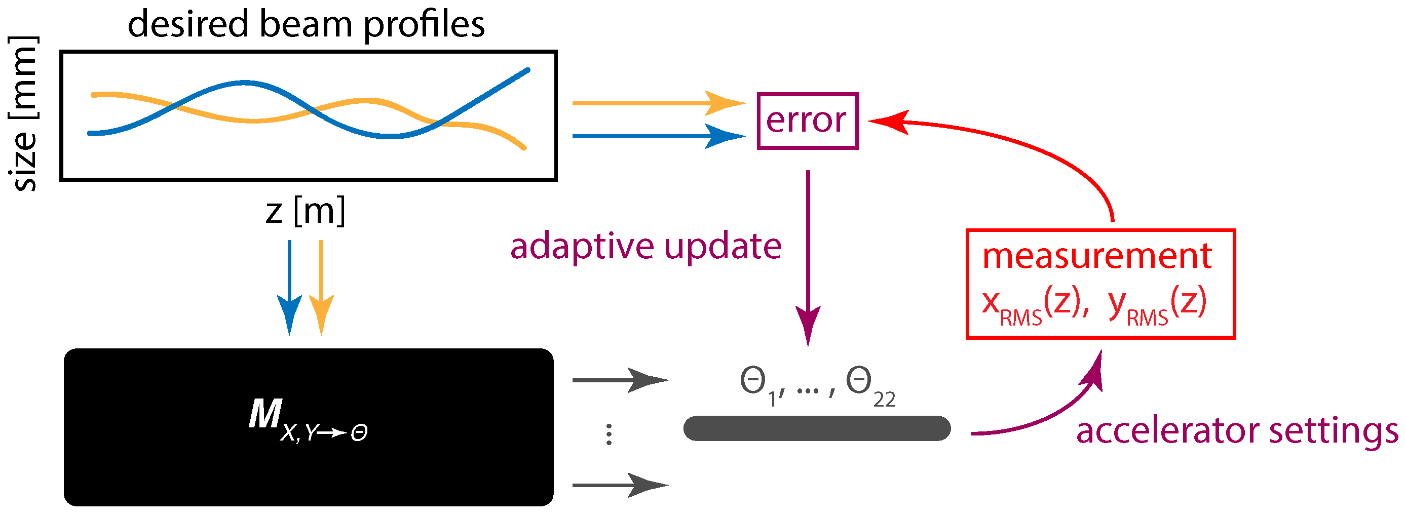
By a similar principal, it is possible to design a second model which can be used to guide feedback control for accelerator tuning, by solving the inverse problem of mapping beam sizes to the quadrupole values that are required to achieve them, referred to as M X , Y Θ . A high level view of such an adaptive control approach is shown in Figure 6. Such a model would require a diagnostic for comparing achieved and desired beam profiles and this type of approach was first demonstrated on the LCLS for automatic control of the LPS whose measurement was available in real time via a transverse deflecting cavity (TCAV) [32].

5. Conclusions

We have shown how combining adaptive model-independent methods with machine learning tools for adaptive ML combines the robustness of adaptive methods to time variation and uncertainty, with the global and extremely fast predictions of complex nonlinear dynamics. The main trick is to introduce extra inputs which may be tuned to modify the ML structure’s predictions based on some measurement. These inputs do not have to be physically measurable quantities, but they should have a physically meaningful effect on the predictions.

Funding

This research was supported by Los Alamos National Laboratory’s Laboratory-Directed Research and Development (LDRD) program by project number 20210595DR.

Data Availability Statement

The data that support the findings of this study are available from the corresponding author upon reasonable request.

Conflicts of Interest

The authors declare no conflict of interest.

References

  1. Friedman, J.; Hastie, T.; Tibshirani, R. The Elements of Statistical Learning; Springer: New York, NY, USA, 2001; Volume 1. [Google Scholar]
  2. Kleene, S.C. Representation of Events in Nerve Nets and Finite Automata; Technical Report; Rand Project Air Force: Santa Monica, CA, USA, 1951. [Google Scholar]
  3. Rasmussen, C.E. Gaussian processes in machine learning. In Summer School on Machine Learning; Springer: Berlin/Heidelberg, Germany, 2003; pp. 63–71. [Google Scholar]
  4. Sutton, R.S.; Barto, A.G. Reinforcement Learning: An Introduction; MIT Press: Cambridge, MA, USA, 2018. [Google Scholar]
  5. Li, Y.; Cheng, W.; Yu, L.H.; Rainer, R. Genetic algorithm enhanced by machine learning in dynamic aperture optimization. Phys. Rev. Accel. Beams 2018, 21, 054601. [Google Scholar] [CrossRef] [Green Version]
  6. Edelen, A.; Neveu, N.; Frey, M.; Huber, Y.; Mayes, C.; Adelmann, A. Machine learning for orders of magnitude speedup in multiobjective optimization of particle accelerator systems. Phys. Rev. Accel. Beams 2020, 23, 044601. [Google Scholar] [CrossRef] [Green Version]
  7. Kranjčević, M.; Riemann, B.; Adelmann, A.; Streun, A. Multiobjective optimization of the dynamic aperture using surrogate models based on artificial neural networks. Phys. Rev. Accel. Beams 2021, 24, 014601. [Google Scholar] [CrossRef]
  8. Emma, C.; Edelen, A.; Hogan, M.; O’Shea, B.; White, G.; Yakimenko, V. Machine learning-based longitudinal phase space prediction of particle accelerators. Phys. Rev. Accel. Beams 2018, 21, 112802. [Google Scholar] [CrossRef] [Green Version]
  9. Hanuka, A.; Emma, C.; Maxwell, T.; Fisher, A.S.; Jacobson, B.; Hogan, M.; Huang, Z. Accurate and confident prediction of electron beam longitudinal properties using spectral virtual diagnostics. Sci. Rep. 2021, 11, 1–10. [Google Scholar] [CrossRef] [PubMed]
  10. Zhu, J.; Chen, Y.; Brinker, F.; Decking, W.; Tomin, S.; Schlarb, H. Deep Learning-Based Autoencoder for Data-Driven Modeling of an RF Photoinjector. arXiv 2021, arXiv:2101.10437. [Google Scholar]
  11. McIntire, M.; Cope, T.; Ermon, S.; Ratner, D. Bayesian optimization of FEL performance at LCLS. In Proceedings of the 7th International Particle Accelerator Conference, Busan, Korea, 8–13 May 2016. [Google Scholar]
  12. Li, Y.; Rainer, R.; Cheng, W. Bayesian approach for linear optics correction. Phys. Rev. Accel. Beams 2019, 22, 012804. [Google Scholar] [CrossRef] [Green Version]
  13. Hao, Y.; Li, Y.; Balcewicz, M.; Neufcourt, L.; Cheng, W. Reconstruction of Storage Ring’s Linear Optics with Bayesian Inference. arXiv 2019, arXiv:1902.11157. [Google Scholar]
  14. Duris, J.; Kennedy, D.; Hanuka, A.; Shtalenkova, J.; Edelen, A.; Baxevanis, P.; Egger, A.; Cope, T.; McIntire, M.; Ermon, S.; et al. Bayesian optimization of a free-electron laser. Phys. Rev. Lett. 2020, 124, 124801. [Google Scholar] [CrossRef] [Green Version]
  15. Li, Y.; Hao, Y.; Cheng, W.; Rainer, R. Analysis of beam position monitor requirements with Bayesian Gaussian regression. arXiv 2019, arXiv:1904.05683. [Google Scholar]
  16. Shalloo, R.; Dann, S.; Gruse, J.N.; Underwood, C.; Antoine, A.; Arran, C.; Backhouse, M.; Baird, C.; Balcazar, M.; Bourgeois, N.; et al. Automation and control of laser wakefield accelerators using Bayesian optimization. Nat. Commun. 2020, 11, 1–8. [Google Scholar] [CrossRef]
  17. Fol, E.; de Portugal, J.C.; Franchetti, G.; Tomás, R. Optics corrections using machine learning in the LHC. In Proceedings of the 2019 International Particle Accelerator Conference, Melbourne, Australia, 19–24 May 2019. [Google Scholar]
  18. Fol, E.; de Portugal, J.C.; Tomás, R. Unsupervised Machine Learning for Detection of Faulty Beam Position Monitors. In Proceedings of the 10th International Particle Accelerator Conference (IPAC’19), Melbourne, Australia, 19–24 May 2019; Volume 2668. [Google Scholar]
  19. Arpaia, P.; Azzopardi, G.; Blanc, F.; Bregliozzi, G.; Buffat, X.; Coyle, L.; Fol, E.; Giordano, F.; Giovannozzi, M.; Pieloni, T.; et al. Machine learning for beam dynamics studies at the CERN Large Hadron Collider. Nucl. Instruments Methods Phys. Res. Sect. A 2021, 985, 164652. [Google Scholar] [CrossRef]
  20. Adelmann, A. On nonintrusive uncertainty quantification and surrogate model construction in particle accelerator modeling. SIAM/ASA J. Uncertain. Quantif. 2019, 7, 383–416. [Google Scholar] [CrossRef]
  21. Hirlaender, S.; Bruchon, N. Model-free and Bayesian Ensembling Model-based Deep Reinforcement Learning for Particle Accelerator Control Demonstrated on the FERMI FEL. arXiv 2020, arXiv:2012.09737. [Google Scholar]
  22. Kain, V.; Hirlander, S.; Goddard, B.; Velotti, F.M.; Della Porta, G.Z.; Bruchon, N.; Valentino, G. Sample-efficient reinforcement learning for CERN accelerator control. Phys. Rev. Accel. Beams 2020, 23, 124801. [Google Scholar] [CrossRef]
  23. Bruchon, N.; Fenu, G.; Gaio, G.; Lonza, M.; O’Shea, F.H.; Pellegrino, F.A.; Salvato, E. Basic reinforcement learning techniques to control the intensity of a seeded free-electron laser. Electronics 2020, 9, 781. [Google Scholar] [CrossRef]
  24. Bruchon, N.; Fenu, G.; Gaio, G.; Lonza, M.; Pellegrino, F.A.; Salvato, E. Toward the application of reinforcement learning to the intensity control of a seeded free-electron laser. In Proceedings of the 2019 23rd International Conference on Mechatronics Technology (ICMT), Salerno, Italy, 23–26 October 2019; pp. 1–6. [Google Scholar]
  25. O’Shea, F.; Bruchon, N.; Gaio, G. Policy gradient methods for free-electron laser and terahertz source optimization and stabilization at the FERMI free-electron laser at Elettra. Phys. Rev. Accel. Beams 2020, 23, 122802. [Google Scholar] [CrossRef]
  26. Scheinker, A.; Krstić, M. Model-Free Stabilization by Extremum Seeking; Springer: Berlin/Heidelberg, Germany, 2017. [Google Scholar]
  27. Dalesio, L.R.; Kozubal, A.; Kraimer, M. EPICS architecture. In Technical Report; Los Alamos National Lab.: Los Alamos, NM, USA, 1991. [Google Scholar]
  28. Agapov, I.; Geloni, G.; Tomin, S.; Zagorodnov, I. OCELOT: A software framework for synchrotron light source and FEL studies. Nucl. Instruments Methods Phys. Res. Sect. A 2014, 768, 151–156. [Google Scholar] [CrossRef]
  29. Scheinker, A.; Bohler, D.; Tomin, S.; Kammering, R.; Zagorodnov, I.; Schlarb, H.; Scholz, M.; Beutner, B.; Decking, W. Model-independent tuning for maximizing free electron laser pulse energy. Phys. Rev. Accel. Beams 2019, 22, 082802. [Google Scholar] [CrossRef] [Green Version]
  30. Scheinker, A.; Hirlaender, S.; Velotti, F.M.; Gessner, S.; Della Porta, G.Z.; Kain, V.; Goddard, B.; Ramjiawan, R. Online multi-objective particle accelerator optimization of the AWAKE electron beam line for simultaneous emittance and orbit control. AIP Adv. 2020, 10, 055320. [Google Scholar] [CrossRef]
  31. Scheinker, A.; Gessner, S. Adaptive method for electron bunch profile prediction. Phys. Rev. Spec. Top. Accel. Beams 2015, 18, 102801. [Google Scholar] [CrossRef] [Green Version]
  32. Scheinker, A.; Edelen, A.; Bohler, D.; Emma, C.; Lutman, A. Demonstration of model-independent control of the longitudinal phase space of electron beams in the linac-coherent light source with femtosecond resolution. Phys. Rev. Lett. 2018, 121, 044801. [Google Scholar] [CrossRef] [Green Version]
  33. Scheinker, A.; Cropp, F.; Paiagua, S.; Filippetto, D. Adaptive deep learning for time-varying systems with hidden parameters: Predicting changing input beam distributions of compact particle accelerators. arXiv 2021, arXiv:2102.10510. [Google Scholar]
  34. Khalil, H.K.; Grizzle, J.W. Nonlinear Systems; Prentice Hall: Upper Saddle River, NJ, USA, 2002; Volume 3. [Google Scholar]
  35. Wu, M. A note on stability of linear time-varying systems. IEEE Trans. Autom. Control 1974, 19, 162. [Google Scholar] [CrossRef]
  36. Wu, M.Y. On stability of linear time-varying systems. Int. J. Syst. Sci. 1984, 15, 137–150. [Google Scholar] [CrossRef]
  37. Mudgett, D.; Morse, A. Adaptive stabilization of linear systems with unknown high-frequency gains. IEEE Trans. Autom. Control 1985, 30, 549–554. [Google Scholar] [CrossRef]
  38. Nussbaum, R.D. Some remarks on a conjecture in parameter adaptive control. Syst. Control Lett. 1983, 3, 243–246. [Google Scholar] [CrossRef]
  39. Scheinker, A. Extremum Seeking for Stabilization. Ph.D. Thesis, University of California San Diego, San Diego, CA, USA, 2012. [Google Scholar]
  40. Scheinker, A.; Krstić, M. Minimum-seeking for CLFs: Universal semiglobally stabilizing feedback under unknown control directions. IEEE Trans. Autom. Control 2012, 58, 1107–1122. [Google Scholar] [CrossRef]
  41. Scheinker, A.; Scheinker, D. Bounded extremum seeking with discontinuous dithers. Automatica 2016, 69, 250–257. [Google Scholar] [CrossRef]
  42. Scheinker, A.; Scheinker, D. Constrained extremum seeking stabilization of systems not affine in control. Int. J. Robust Nonlinear Control 2018, 28, 568–581. [Google Scholar] [CrossRef]
  43. Scheinker, A.; Scheinker, D. Extremum seeking for optimal control problems with unknown time-varying systems and unknown objective functions. Int. J. Adapt. Control. Signal Process. 2020. [Google Scholar] [CrossRef]
  44. Bellman, R. Dynamic programming and Lagrange multipliers. Proc. Natl. Acad. Sci. USA 1956, 42, 767. [Google Scholar] [CrossRef] [PubMed] [Green Version]
  45. Kirk, D.E. Optimal Control Theory: An Introduction; Courier Corporation: Chelmsford, MA, USA, 2004. [Google Scholar]
  46. Lewis, F.L.; Vrabie, D.; Syrmos, V.L. Optimal Control; John Wiley & Sons: Hoboken, NJ, USA, 2012. [Google Scholar]
  47. Silver, D.; Hubert, T.; Schrittwieser, J.; Antonoglou, I.; Lai, M.; Guez, A.; Lanctot, M.; Sifre, L.; Kumaran, D.; Graepel, T.; et al. A general reinforcement learning algorithm that masters chess, shogi, and Go through self-play. Science 2018, 362, 1140–1144. [Google Scholar] [CrossRef] [PubMed] [Green Version]
  48. Kapchinskij, I.; Vladimirskij, V. Limitations of proton beam current in a strong focusing linear accelerator associated with the beam space charge. In Proceedings of the 2nd International Conference on High Energy Accelerators and Instrumentation, Geneva, Switzerland, 14–19 September 1959. [Google Scholar]
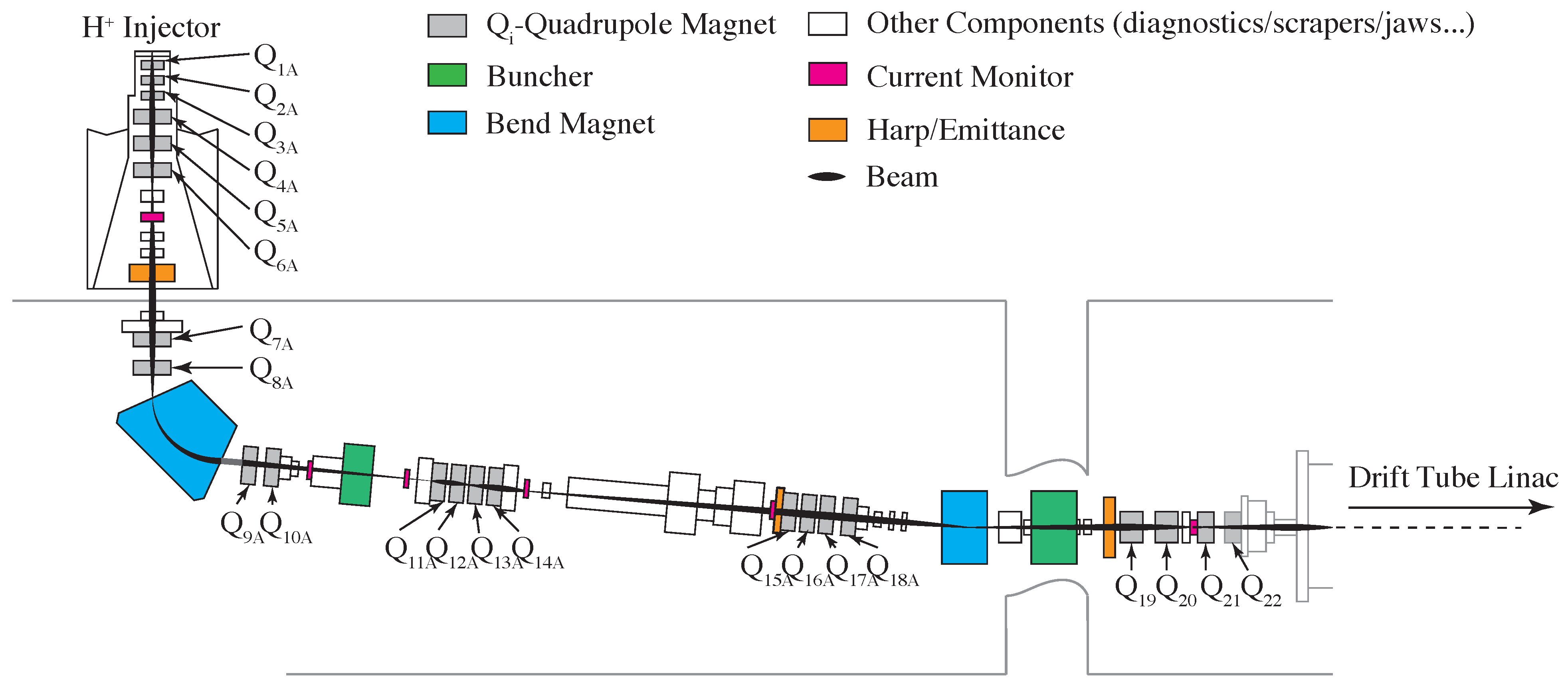
Figure 1. An overview of the LANSCE H + low energy beam transport and its 22 quadrupole magnets is shown.
Information 12 00161 g001
Figure 2. A high level view of the adaptive NN diagnostic M Θ X , Y is shown.
Information 12 00161 g002
Figure 3. Comparison of NN predictions when using the correct initial conditions and when using the mean value.
Information 12 00161 g003
Figure 4. Comparison of the best (left), average (midddle) and worst (right) NN predictions for beam envelopes.
Information 12 00161 g004
Figure 5. The adaptive diagnostic is able to track the time-varying beam in real time by tuning the input beam sizes based only on the error measured at the end of the beamline. The left most subplot shows the changing initial beam sizes ad how they are tracked. The middle subplot shows the growth of the error without adaptive tuning and with ES. The right most plot shows all of the trajectories overlapped as they are tracked by the adaptive diagnostic.
Information 12 00161 g005
Figure 6. A high level view of the adaptive NN controller M X , Y Θ is shown.
Information 12 00161 g006
Publisher’s Note: MDPI stays neutral with regard to jurisdictional claims in published maps and institutional affiliations.