To facilitate mathematical analysis, we abstract real-world individuals as nodes and abstract the relationships between nodes as edges, and nodes and edges together form the graph. However, due to the diverse relationships between nodes in the real world, it is difficult for the method to learn accurate node representations, so it is difficult to obtain accurate node clustering results.
In response to the above problems, we propose the Dual-Channel Heterogeneous Graph Network for author name disambiguation. The method learns the semantic information of the papers through the textual information, including the title, the journal/conference that published the paper, author institution, the abstract of the paper, and keywords. Then, fastText is used to generate the semantic representation vector of each paper, and then the semantic similarity matrix of the paper is obtained. A heterogeneous graph network based on the paper is constructed, and the meta-path-based random walk algorithm is used to obtain the relationship features of the paper, the relationship vector of the paper, and the relationship similarity matrix. Finally, the semantic similarity matrix and the relational similarity matrix are merged, and the similarity matrix is clustered by DBSCAN. In this way, papers by different authors can be allocated to different clusters, thus achieving author name disambiguation. Because our method does not have strict requirements for the dataset, it is suitable for academic paper digital libraries in different organizations or different public datasets, such as the DBLP digital library dataset or Aminer digital library dataset. The framework is shown in
Figure 2.
4.1. Use FastText to Construct Semantic Representation Vector
The purpose of semantic representation learning is to obtain the vector representation of the semantic information based on Cai et al. [
16] and Shi et al. [
17]. For this purpose, we used fastText [
18], which was trained on a large-scale academic paper database through unsupervised learning to obtain a word vector model. In order to obtain the semantic representation vector of the entire article, it is necessary to obtain the vector representation of the entire article by performing a weighted summation on the required word vectors selected in the word vector model.
Construction of the training corpus. Before training the word vector model through fastText, a corpus suitable for training needs to be constructed. In order to improve the effectiveness of the fastText training word vector model, this training corpus should include a large amount of data. Our research is based on the AMiner open-source dataset, which has a small amount of data. In order to improve the result of the fastText training word vector model, the amount of data in this training corpus needs to be further expanded. The data that we use include two parts. One part comes from the collected academic paper dataset, about 200,000 academic papers; the other part comes from the DBLP dataset, about 1.4 million academic papers.
First, the text information of each article in the above-mentioned dataset is extracted into a text corpus. The title, journal/conference, author’s institution, keywords, abstract, and publication year of each paper are included in its textual information. The text information is saved in a text file as a training corpus. Then, the fastText model is used to train the word vector model.
Training parameter settings. After comparing the effects of the word vector model trained under multiple sets of different parameter settings in the disambiguation experiment, a set of relatively optimal parameter setting schemes was obtained. The specific training parameters are shown in
Table 1.
As shown in the table, the dimension of the semantic vector generated by fastText is set to 100. The training model selected in the training process is the CBOW [
19] model. The
algorithm is used for optimization, the context word window size is set to 5, and the minimum and maximum numbers of training characters are set to 3 and 6, respectively. After the training is completed, a word vector model file is obtained, mainly composed of “word-corresponding word vector and character-corresponding character word vector” for semantic vector generation.
The fastText algorithm is used to train text word vector models not only because of its ability to train word vectors at word granularity but, more importantly, because of its ability to train word vectors at character granularity [
20]. For example, the word “matter”, assuming that the 3-gram feature is used, can be represented as five 3-gram features.
Using
n-gram has the following advantages: (1) It generates better word vectors for rare words. According to the above character-level
n-gram, even if this word appears very few times, the characters that make up the word and other words have shared parts, so this can optimize the generated word vector. (2) Even if the word does not appear in the training corpus, the word vector of the word can still be constructed from the character-level
n-gram [
21]. (3)
n-gram can allow the method to learn word order information. If
n-gram is not considered, the information contained in the word order cannot be considered, which can also be understood as context information. Therefore,
n-gram is used to associate several adjacent words, which allows the method to maintain word order information during training.
Semantic matrix of academic papers. First, text information, such as the title, published journal/conference, author’s institution, keywords, abstract, and publication year, is separated by spaces to synthesize the paragraph representing this paper. Then, the text information is processed to lowercase letters; various non-letter symbols, extra spaces, stop words, and words with a length less than 2 are removed, and spaces are used for word segmentation.
Through the above-trained fastText word vector model, a corresponding word vector is generated for each word in the processed text, and each word vector is weighted to obtain a semantic representation vector representing each paper. The reason for assigning different weights to each word vector is that the importance of different words varies. It is generally observed that certain words are only used in specific fields and appear less frequently. The importance of some common words is generally lower than that of some specific words. We counted the words in the AMiner dataset. After removing the stop words, the dataset has nearly 370,000 words, which constitute the training corpus. After further statistical analysis, we found that most words appear less than 10 times in the dataset. The results are shown in
Table 2.
Finally, the cosine similarity between the two papers is calculated by the obtained semantic vector of academic papers. This results in the semantic similarity matrix of papers.
4.2. Use Heterogeneous Graph to Construct Relational Representation Vector
The academic paper contains semantic information and information about the co-authors and their institutions, which means that a social network relationship also exists between academic papers. Exploring this kind of network relationship and combining it with semantic information is the key to name disambiguation. We used the related information to obtain a relationship vector representation for subsequent research on name disambiguation.
The process of obtaining the relationship representation vector of each paper is mainly divided into the following two steps: (1) Construct a heterogeneous graph network of the paper using the author’s information, author’s institution information, and the journal or conference where the paper is published. (2) After constructing the heterogeneous graph network, use the meta-path random walk method to learn the representation vector of each paper [
22]. There has been much research and progress related to heterogeneous graph networks. Our work was influenced by related research on methods such as metapath2vec [
23] and Hin2Vec [
24], and we adopted a Hin2Vec-based heterogeneous graph network [
25] to obtain the relationship vector representation of the paper. In contrast to the way that metapath2vec walks according to the given meta-path, the HIN2Vec model is completely based on a random walk, and it can walk as long as the nodes are connected.
Constructing the heterogeneous graph network. First, the author’s name to be disambiguated is extracted; then, the relationship between all published academic papers corresponding to this name is extracted, and a heterogeneous graph network is constructed. Python is used to construct the adjacency matrix that represents the node relationship. If there is a connection between nodes
i and
j, then in the adjacency matrix, the value in row
i and column
j is 1. If there is no connection between nodes
i and
j, then the value in row
i and column
j is 0. The connection between the node and itself is not considered; that is, the connection between the node and itself is 0. We constructed a heterogeneous graph network containing one type of node: academic paper (
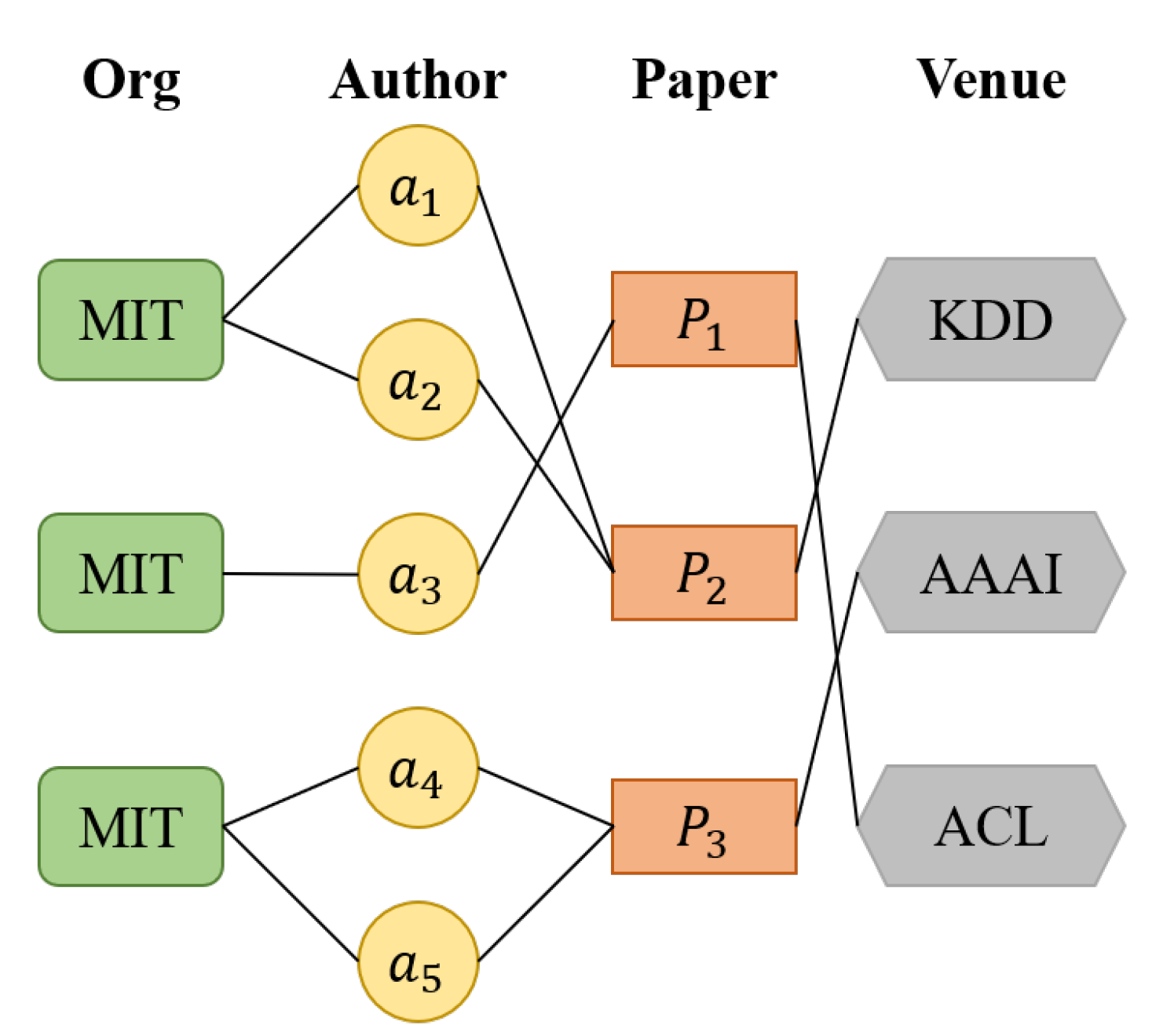
). That is, each academic paper represents a node in the heterogeneous graph network. The network also contains three types of edges: co-author, author’s organization (Co-Org), and journal that published the paper (Co-Venue). The heterogeneous graph network that we constructed is shown in
Figure 3.
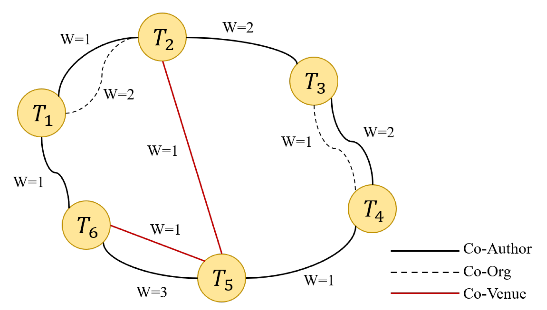
If two papers contain co-authors other than the author to be disambiguated, we construct a Co-Author edge between the two papers in the heterogeneous graph network. The weight
W of the edge represents the number of co-authors other than the authors to be disambiguated. For example, in
Figure 3, two papers
and
have a co-author; then, an edge named Co-Author is constructed between them, and the weight
W of the edge is 1.
Similarly, in the heterogeneous graph network, Co-Org represents the similarity relationship between co-authors’ institutions. The weight
W of the edge represents the number of words in common in the names of the two institutions. For example, in
Figure 3, the institutional information of two papers
and
has a common word that is not a stop word, so an edge named Co-Org is constructed between the two papers, and its
W is 1. Co-Venue type edges are constructed in the same way as Co-Org edges, so we do not repeat the description.
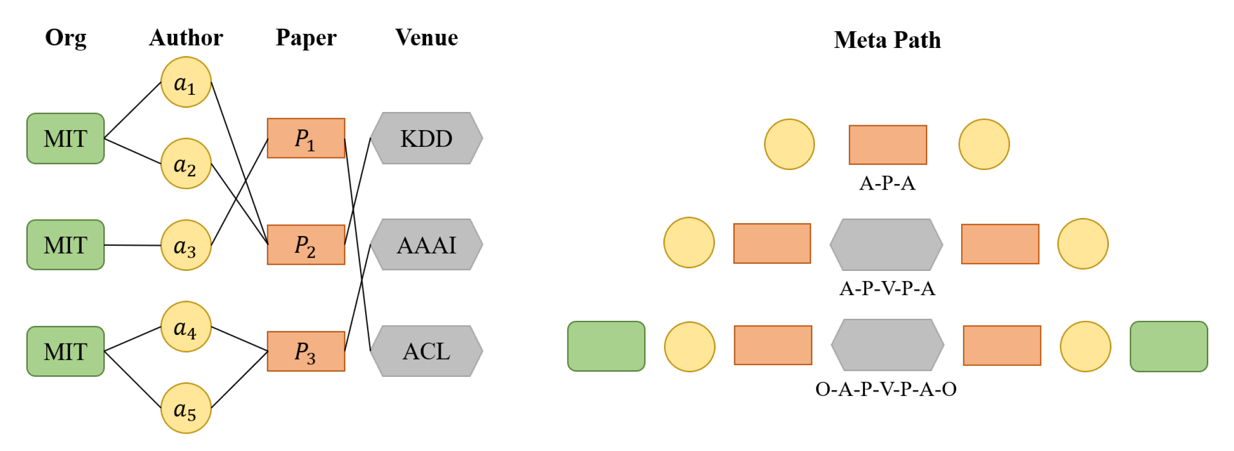
Random walk of meta-paths in the heterogeneous graph network. The meta-path can be defined in the following form.
represents the pathset from vertex
to vertex
.
Taking the heterogeneous graph network in
Figure 4 as an example, the vertex types in the network are Org, Author, Paper, and Venue. There are several types of meta-paths: (1) “Author-Paper-Author”, (2) “Author-Paper-Venue-Paper-Author”, and (3) “Org-Author-Paper-Venue-Paper-Author-Org”.
After constructing the heterogeneous information network, we generate a pathset composed of the paper’s ID based on the random walk of meta-paths. Then, the paper’s ID is used as the input of the Hin2Vec model. Finally, the corresponding relationship representation vector for each ID is obtained. The relationship vector of papers indicates that the relationship between different papers has been learned, and the similarity between the two papers can be obtained by calculating the cosine similarity.
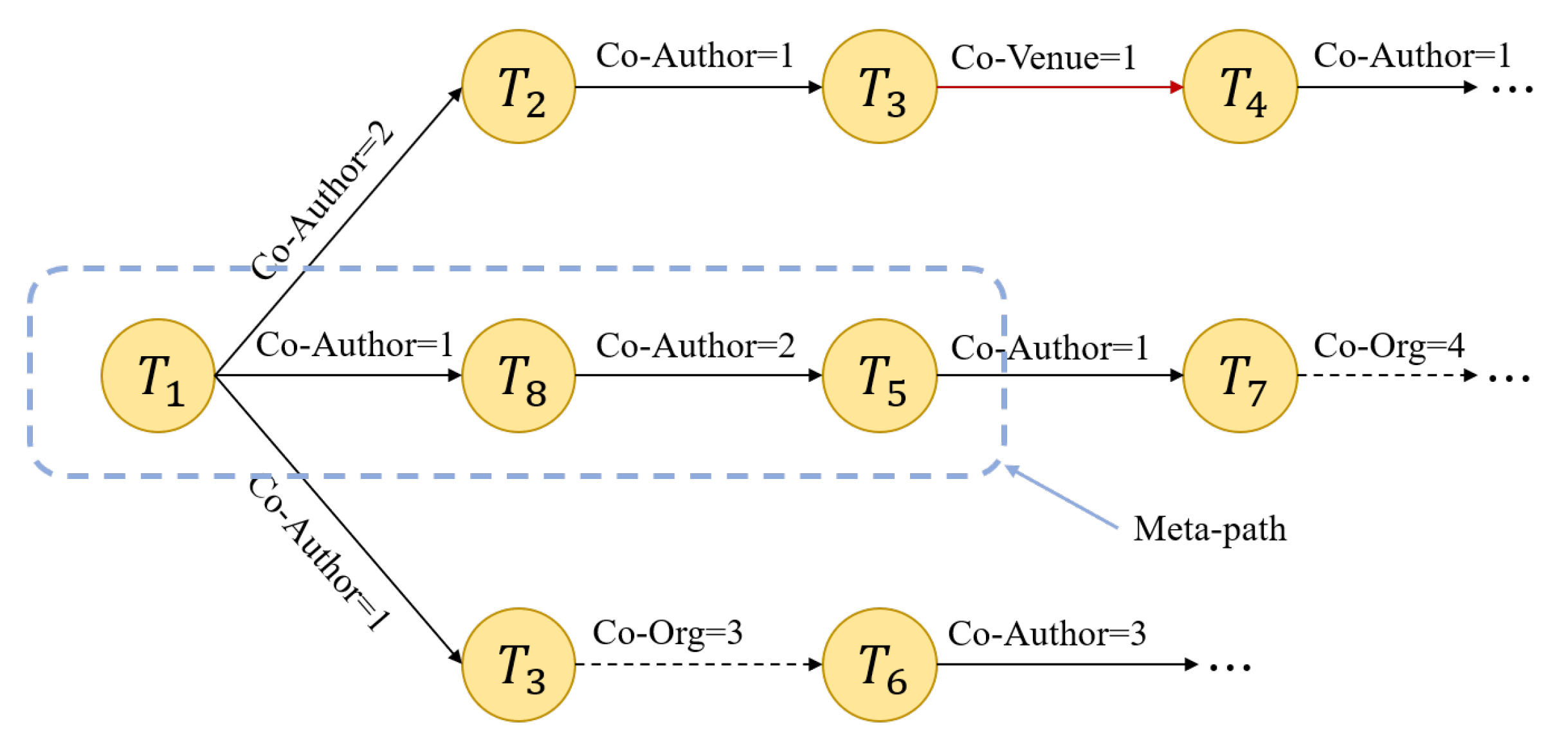
In a random walk, a node is randomly selected in the network as the initial node, and the process then walks along the edge connected to the initial node to the next node in the network. The number of nodes, also called the path length, needs to be set in advance of the walk. After the random walk, the path set is saved for subsequent training. The random walk based on the meta-path refers to a random walk on the edge of the network. It is not completely random but can be guided by the specified meta-path [
26]. In randomly selecting the next node, we consider the weight of the edge in the network. The greater the weight, the closer the relationship between the two nodes, and the greater the probability that the node will walk along this edge. We stipulate that the probability and the weight are proportional. For example, in
Figure 5,
is selected as the initial node, the next relationship of the random walk is “Co-Author”, and the three nodes that have this relationship with
are
,
, and
. According to the edge weight, the probability of walking from
to
is 2/3, the probability of walking to
is 1/4, and the probability of walking to
is 1/4.
The specific random walk process selects the next node according to the edge specified by the current meta-path; it randomly selects a node connected to the current node through this edge as the next node. In each path, the meta-path is repeatedly sampled several times. That is, the last node of the previous meta-path is used as the first node of the next meta-path. Iterations are continuously carried out until a certain number of rounds is reached, after which another node is selected as the initial node to walk. Finally, several paths are generated, where the node of each path is the ID of the paper, and each path is stored for the generation of the relation vector.
There is no guarantee that all three types of edges and two types of nodes exist in a heterogeneous graph network. For example, in a particular paper, authors other than the author to be disambiguated may not appear, so then the “Co-Author” relationship of this paper is missing. When this happens, other random walk strategies need to be adopted. For example, a random walk can be performed based on the “Co-Org” relationship or the “Co-Venue” relationship. When a node cannot construct any type of edge with other nodes, we classify it as an isolated node, and we save it separately for subsequent processing.
Academic paper relational representation learning. When obtaining the relation vector representation of each paper, nodes
and
and their relation
R are subjected to one-hot encoding as the input of Hin2Vec, and the vector representation of the node is learned by maximizing the relation
R. The objective function is defined as
O,
where
D represents the training dataset, and
and
represent two nodes in the heterogeneous graph network.
R represents the relationship between the two nodes. During training, the training dataset is given in the following form:
where
represents the probability that there is a relationship
R between nodes
and
in the heterogeneous graph network, and
is a binary value. When it is equal to 1, it means that the objective function is maximized. It is simplified to:
After learning the vector representation of each node in the heterogeneous graph network, the cosine similarity between every two papers is calculated to obtain the relationship similarity matrix. Hin2Vec learns the node vector representation using the parameter settings shown in
Table 3.
For each node, the set number of walks is five, and the maximum length of each walk is 20. In the representation learning stage, the model is trained five times, each training sample is 20 groups, the vector representation of each node is learned, and the embedding vector is 100 dimensions.
4.3. Use DBSCAN for Node Clustering
Clustering is performed through the semantic similarity matrix and the relationship similarity matrix obtained in the previous two sections. This section describes how the DBSCAN clustering algorithm is used to cluster academic papers.
DBSCAN clustering. We add the relationship similarity matrix and the semantic similarity matrix to find the average value and obtain the final academic paper similarity matrix.
The unsupervised clustering algorithm DBSCAN [
27] is used for disambiguation, and papers by the same author are clustered into one class. The DBSCAN clustering algorithm does not require the number of clusters to be specified in advance and is not sensitive to outliers in the data. Because we cannot accurately obtain the actual value of the number of real authors under the one name, we cannot determine the number of clusters in the final cluster, but DBSCAN avoids this problem. The parameter settings of DBSCAN are shown in
Table 4.
Matching of isolated papers. After the above DBSCAN clustering, some clusters can be obtained, and each cluster contains academic papers belonging to the same author. In addition, for the isolated papers that cannot establish a relationship with any node, the similarity feature matching method is used to redistribute them to clusters that have already been generated. The remaining isolated papers that cannot be matched are treated as new clusters.
An isolated paper arises because this part of the paper has too little feature information, and its similarity to other papers is relatively low, or the paper itself belongs to an author who has published few papers. Using a feature-based matching approach works better for this type of paper. Therefore, the matching method for this scenario is divided into the following two steps.
Step 1: Each paper in the isolated paper set is compared with other papers in the dataset through feature matching, and the paper with the highest similarity is identified. If the feature similarity between the two documents is not less than the threshold , then the former is allocated to the cluster that contains the latter. Otherwise, the former is individually classified as a new cluster.
Step 2: After completing feature matching for each isolated paper, the papers in new clusters are compared. If the similarity between the two papers is not less than the threshold , then the two papers belong to the same cluster. Otherwise, the two papers do not belong to the same cluster. This step is completed until matching is complete.
Specifically, when matching the feature similarity of an isolated paper set, first, the stop words are removed from the title, keywords, and abstract, and then a new piece of text is synthesized. The Jaccard Index of the text of papers
and
is calculated. The formula is defined as:
where
X and
Y represent the bag of words in papers
and
, and the result range is (0, 1). After the above processing, the papers in the isolated paper set can also be assigned to their respective clusters, thereby obtaining the clustering disambiguation results of all academic papers.


