LED-Lidar Echo Denoising Based on Adaptive PSO-VMD

Abstract

LED (light-emitting diode)-lidar (light detection and ranging) has gradually been focused on by researchers because of its characteristics of low power, high stability, and safety to human eyes. However, LED-lidar systems are easily disturbed by background light noise. Echo signal denoising is an essential work that directly affects the measurement accuracy of the LED-lidar system. The traditional variational modal decomposition (VMD) method in lidar signal denoising relies on practical experience to optimize the critical parameters of quadratic penalty factor α and the number of intrinsic mode function (IMF) components K globally, which is hard to denoise effectively. For this problem, a denoising method based on VMD with the adaptive weighted particle swarm optimization (PSO) is proposed in this work. The PSO-VMD method adaptively adjusts the weight value ω for different lidar echo signals and optimizes of the parameters α and K globally. The LED-lidar echo signals are denoised by moving average, VMD, and PSO-VMD. Using the denoised echo signals, the range compensation waveforms and the extinction coefficients are derived. The results show that the PSO-VMD denoised echo signal has the highest R-square value of 0.9972 and the minimum standard deviation value of 5.7369, while the values of r-square and standard deviation of the echo signal denoised by moving average and VMD method are 0.9902, 9.7450, 0.9945, and 7.3588, respectively. The derived distance compensation waveforms and extinction coefficients based on the PSO-VMD denoising have better stability than those based on the moving average and VMD denoising.

1. Introduction

As a typical optical remote sensing technology [1], lidar (light detection and ranging) is widely applied in environmental monitoring, geographic mapping, hazardous gas detection, and other applications [2,3,4,5,6,7,8,9,10,11]. With the development of industrialization and the increasingly severe global environmental problems, the environmental monitoring applications of lidar, especially atmospheric aerosol monitoring, have been widely studied by researchers. Compared with chemical sensor measurement techniques, lidar has the advantages of a wide measurement range, high accuracy, and the ability to obtain the spatial distribution of the aerosol by scanning. These advantages benefit from the collimation and high-power characteristics of the laser light source. However, the high-quality laser is expensive, bulky, has a high power consumption, and is strict for the use of the environment. More importantly, the use of high-power lasers in the central part of the city, urban buildings, and densely populated spaces has safety risks to human eyes. These factors make lidar mainly used in developed countries or advanced regions, and its use environment is limited in laboratories and sparsely populated areas. Lidar is challenging to be applied in densely populated areas of cities for various types of monitoring applications.

The safety of the light source, the compactness of the lidar device, and the power consumption are essential factors in close- and small-range aerosol monitoring applications, such as dust monitoring on factory floors, exhaust gas emission monitoring in factories, flammable and explosive gas monitoring in hydrogen energy station, etc. For these reasons, this study focuses on the lidar system with LED (light-emitting diode) as the light source. Although LED is inferior to laser in terms of collimation, emission power, and spectral line width, it has many advantages that lasers do not have: low price, low energy consumption, low-voltage working power, high stability, high applicability, high flexibility in application, and safety to human eyes. For these advantages, LED is widely applied in various scenarios.

The Shiina’s group from Chiba University started the application of LED-lidar earlier. Several prototypes such as in-line-type and dual-axis-type LED-lidar were created by their team [12,13]. Their team applied the LED-lidar system in surface atmospheric measurements and successfully acquired close-range atmospheric echo signals. However, the LED light source is difficult to collimate, and its radiated power decreases rapidly with increasing distance, which makes the LED-lidar system vulnerable to the influence of background light noise. It is challenging to meet the high-precision measurement in spatial resolution and dynamic range. To improve the applicability of LED-lidar in various applications, echo signal denoising is vital work. However, the difference in power and collimation between LED-lidar and traditional lidar makes the dynamic range of LED-lidar echo signal much smaller than that of traditional lidar. The simple denoising method, such as moving average, cannot remove the noise of LED-lidar echo well, even wrongly removing the LED-lidar echo signal as background noise. Therefore, an effective denoising method can improve the accuracy of aerosol monitoring with LED-lidar, especially in long distances with a low value of signal-to-noise ratio (SNR).

The lidar echo is a nonlinear and nonstationary signal. Nonlinear denoising algorithms such as Kalman filter (KF), wavelet transform (WT), empirical mode decomposition (EMD), and other algorithms have been applied in the application of lidar denoising. KF is a recursive algorithm based on minimum mean square error, which can process nonstationary and multidimensional signals from time-varying systems. However, the calculation accuracy of this method decreases significantly when the signals change dramatically [14]. WT can decompose signals into different frequency components through multiscale analysis, which has good localization characteristics in the time–frequency domain. However, it has poor adaptability due to the selection of the wavelet basis function [15]. EMD made up for the inadequacy of WT, which has good adaptability and can reflect the characteristics of the specific frequency of the signal. However, it has the endpoint effect and modal aliasing problems due to the recursive mode decomposition characteristics of the EMD method, which hinders the separation of the echo signal from noise [16,17]. For these reasons, variational mode decomposition (VMD) is proposed to solve the problem above. VMD can effectively avoid the problems of modal aliasing and endpoint effect caused by EMD. However, it is found that the quadratic penalty factor α and the number of intrinsic mode function (IMF) components K have a significant influence on its decomposition effect [18]. The traditional VMD method combines the local optimal solution of α and K by experimental method and empirical method, respectively [19]. However, the combination of local optimal solutions is challenging to achieve the global optimal effect because of the correlation between α and K parameters. To increase the denoising effect of VMD in LED-lidar applications, an algorithm that can optimize critical parameter combinations [α, K] is needed [20].

Particle swarm optimization (PSO) is an intelligent algorithm with global optimization ability [21]. The algorithm finds the optimal solution through cooperation and information sharing among individuals in a group. It has been widely used in function optimization, neural network training, fuzzy system control, and other applications of genetic algorithms due to its simple operation and fast convergence [22,23]. However, for traditional PSO, it is difficult to achieve local optimization and global optimization synchronously because the weight parameter ω is set as a constant. It can obtain a better global optimization effect if the ω can be assigned dynamically in different original signals.

In this paper, the parameters [α, K] of VMD are optimized by the PSO algorithm with adaptive weights, and the VMD is used to denoise the LED-lidar echo signals. To estimate the effectiveness of the PSO-VMD algorithm, the same LED-lidar atmospheric echo signals are denoised with the moving average method, the VMD algorithm, and the PSO-VMD algorithm, respectively, and the denoised results are compared. The improved effect of denoising from the PSO-VMD is also estimated from the calculation result of the extinction coefficient.

The main content of this paper is as follows: Section 1 presents the background of LED-lidar and the algorithm of lidar signal denoising. Section 2 offers the PSO-VMD method. Section 3 introduces the LED-lidar system, data acquisition, and calculation process of extinction coefficient. Section 4 presents the results of LED-lidar signal denoising with PSO-VMD and the other methods. Section 5 is the conclusion.

2. Theory

2.1. VMD

VMD is a new multicomponent signal decomposition algorithm based on Wiener filtering, Hilbert transform, and outlier demodulation [18]. VMD can decompose a signal $f\left(t\right)$ into K discrete modes ${\mu }_k\left(k=1,2,3\cdots ,K\right)$. ${\mu }_k$ are amplitude–frequency modulated (AM-FM) signals, and their bandwidths have sparsity in the frequency domain, effectively suppressing the modal aliasing that occurs in EMD. Each ${\mu }_k$ is compacted around the center frequency, and its bandwidth can be obtained by Gaussian smoothing demodulation. The constrained variational problem in the VMD can be expressed as:

$$\begin{gathered} \left\{\underset{\left\{{\mu }_k\right\},\left\{{\omega }_k\right\}}{\min }\left\{{\displaystyle \sum }_k\Vert {\partial }_t\left[\left(\delta \left(t\right)+\frac{j}{\pi t}\right){\ast \mu }_k\left(t\right)\right]e^{-{j\omega }_{k}t}\Vert {}_2^2\right\}\right\} \\ \mathrm{S}.\mathrm{t}.{\displaystyle \sum }_k{\mu }_k\left(t\right)=f \end{gathered}$$

(1)

$\left\{{\mu }_k\right\}=\left\{{\mu }_1,{\mu }_2\cdots {\mu }_K\right\}$ and $\left\{{\omega }_k\right\}=\left\{{\omega }_1,{\omega }_{2\cdots }{\omega }_K\right\}$ are the sets of the decomposed modes and their central frequencies, respectively. The quadratic penalty parameter $\alpha$ and the Lagrange multiplier operator $\lambda \left(t\right)$ are introduced to obtain the solution to the constrained variational problem in Equation (1). The augmented Lagrangian function is expressed as:

$$\begin{gathered} L\left(\left\{{\mu }_k\right\},\left\{{\omega }_k\right\},\lambda \right)=\alpha {\displaystyle \sum }_k\Vert {\partial }_t\left[\left(\delta \left(t\right)+\frac{j}{\pi t}\right)\ast {\mu }_k\left(t\right)\right]e^{-j{\omega }_{k}t}\Vert {}_2^2 \\ +\Vert f\left(t\right)-{\displaystyle \sum }_k{\mu }_k{\left(t\right)\Vert }_2^2+\lambda \left(t\right),f\left(t\right)-{\displaystyle \sum }_k{\mu }_k\left(t\right) \end{gathered}$$

(2)

The saddle point of Equation (2) can be obtained by the alternating direction method of multipliers. Then ${\mu }_k$, ${\omega }_k$, and $\lambda$ can be updated iteratively in the frequency domain.

The steps of VMD are as follows:

(a)

Initializing $\left\{{\mu }_k^1\right\}$, $\left\{{\omega }_k^1\right\}$, ${\lambda }^1$ and setting $n=0$;

(b)

Updating ${\mu }_k$ and ${\omega }_k$ iteratively by Equations (3) and (4), respectively:

$${\mu }_k^{n+1}\left(\omega \right)=\frac{f\left(\omega \right)-{{\displaystyle \sum }}_{i\ne k}{\mu }_i\left(\omega \right)+\frac{\lambda \left(\omega \right)}{2}}{1+2\alpha \left(\omega -w_k\right)}$$

(3)

$${\omega }_k^{n+1}=\frac{{{\displaystyle \int }}_0^{\infty }\omega {\left|{\mu }_k\left(\omega \right)\right|}^{2}d\omega }{{{\displaystyle \int }}_0^{\infty }{\left|{\mu }_k\left(\omega \right)\right|}^{2}d\omega }$$

(4)

(c)

Updating $\lambda$ according to Equation (5):

$${\lambda }^{n+1}\left(\omega \right)\leftarrow {\lambda }^n\left(\omega \right)+\tau \left[f\left(\omega \right)-{\displaystyle \sum }_k{\mu }_k^{n+1}\left(\omega \right)\right]$$

(5)

(d)

Repeating steps (b)–(c) until the iteration result is satisfied the ending condition:

$${\displaystyle \sum }_k\Vert {\mu }_k^{n+1}-{\mu }_k^n\Vert {}_2^2/\Vert {\mu }_k^n\Vert {}_2^2<\epsilon$$

(6)

where $\epsilon$ is the discriminant accuracy, and $\epsilon >0$.

(e)

Outputting K modal components.

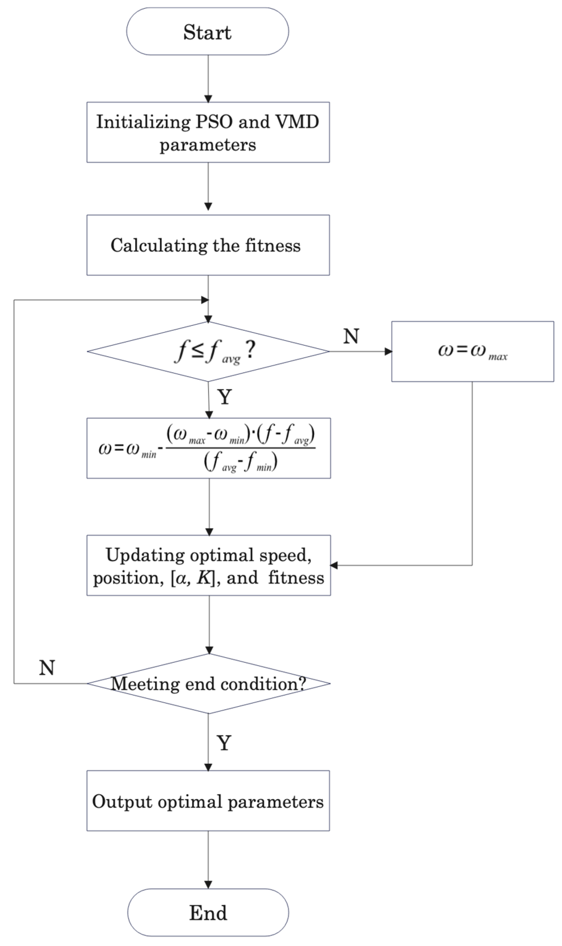
2.2. PSO

PSO is an algorithm for global optimization of key parameters, and determination of the fitness function is a key step in the PSO algorithm [21]. The fitness function is updated with the change in particle position, and the updated direction of the particle is dependent on the value of the fitness function. The minimum of the envelope entropy is used as the fitness function, which represents the sparsity of the original signal. The envelope entropy is more prominent when the signal-to-noise power ratio is small. On the other hand, the envelope entropy value is smaller when the signal-to-noise power ratio is significant. The envelope entropy $E_p$ can be expressed as:

$$E_p=-{\displaystyle \sum }_{j=1}^N{p}_j\lg \left(p_j\right)$$

(7)

$$p_j=\frac{a\left(j\right)}{{{\displaystyle \sum }}_{j=1}^N{a}_j}$$

(8)

$$a\left(j\right)=\sqrt{x^2\left(j\right)+{\widehat{x}}^2\left(j\right)}$$

(9)

where $p_j$ is the sequence of probability distributions of $a\left(j\right)$; $a\left(j\right)$ is the envelope obtained from the Hilbert demodulation of $x\left(j\right)$.

The weight parameter ω in the traditional PSO algorithm is set as a constant, which easily leads to the problem of local optima. An adaptive nonlinear dynamic inertial weight coefficient ω, as shown in Equation (10), was adopted in the PSO algorithm to optimize the VMD parameters in this study. The flowchart of the adaptive-weight PSO-VMD is shown in Figure 1. The nonlinear dynamic inertial weight is closely related to the global optima, which can vary with the position of particles, and solve the problem of local optima.

$$\omega =\left\{\begin{array}{c} {\omega }_{min}-\frac{\left({\omega }_{max}-{\omega }_{min}\right)\ast \left(f-f_{avg}\right)}{f_{avg}-f_{min}}, f\le f_{avg}\\ {\omega }_{max} , f>f_{avg}\end{array}\right.$$

(10)

where $f$ is the fitness function, which is $E_p$ mentioned in Equation (7); $f_{avg}$ is the average of the fitness function; and $f_{min}$ is the minimum of the fitness function.

The calculation steps of PSO-VMD are as follows:

(a)

Parameter initialization: the main parameters are the population size, the maximum number of iterations, and the search range of the parameters α and K.

(b)

Updating iteratively: using the minimum of envelope entropy as the fitness function and updating the velocity and position of the population iteratively.

(c)

Determining the adaptive nonlinear dynamic inertial weight ω according to the most calculated current envelope entropy and the mean value of envelope entropy.

(d)

Update the new optimal [α, K] and the minimum envelope entropy if the new calculated envelope entropy is smaller than the minimum of the envelope entropy.

(e)

Repeat steps (b)–(d) until the maximum number of iterations as well as the minimum envelope entropy is determined; output the optimal parameters α and K.

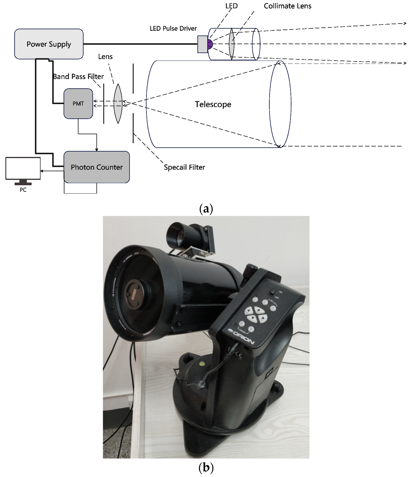
3. LED-Lidar System and Signal Processing

3.1. LED-Lidar System

A biaxial type of LED-lidar was used in this study [13]. Figure 2 shows the schematic diagram of LED-lidar and its prototype used in this study. The LED pulse driver provides a pulse with a high frequency of 500 kHz and a pulse width of 10 ns, which is used to drive a high-power LED with a wavelength of 395 nm. The LED has an average power of 3.82 mW and a peak power of 764 mW. The beam from LED is collimated by a combination of a silicone lens and a Fresnel lens and emitted from the transmitter with a diffusion angle of 12.5 mrad. The transmitted beam generates the backscattering light while propagating in the aerosol. The backscattering light is focused by the telescope and collimating lens. After filtering with a special filter and bandpass filter, the focused light is converted to electrical signals by a photomultiplier tube (PMT). The photon counter is used for the integral operation to make the LED-lidar echo signal stable. The LED-lidar echo samples used in this study are obtained from the photon counter with 10⁵ integrals.

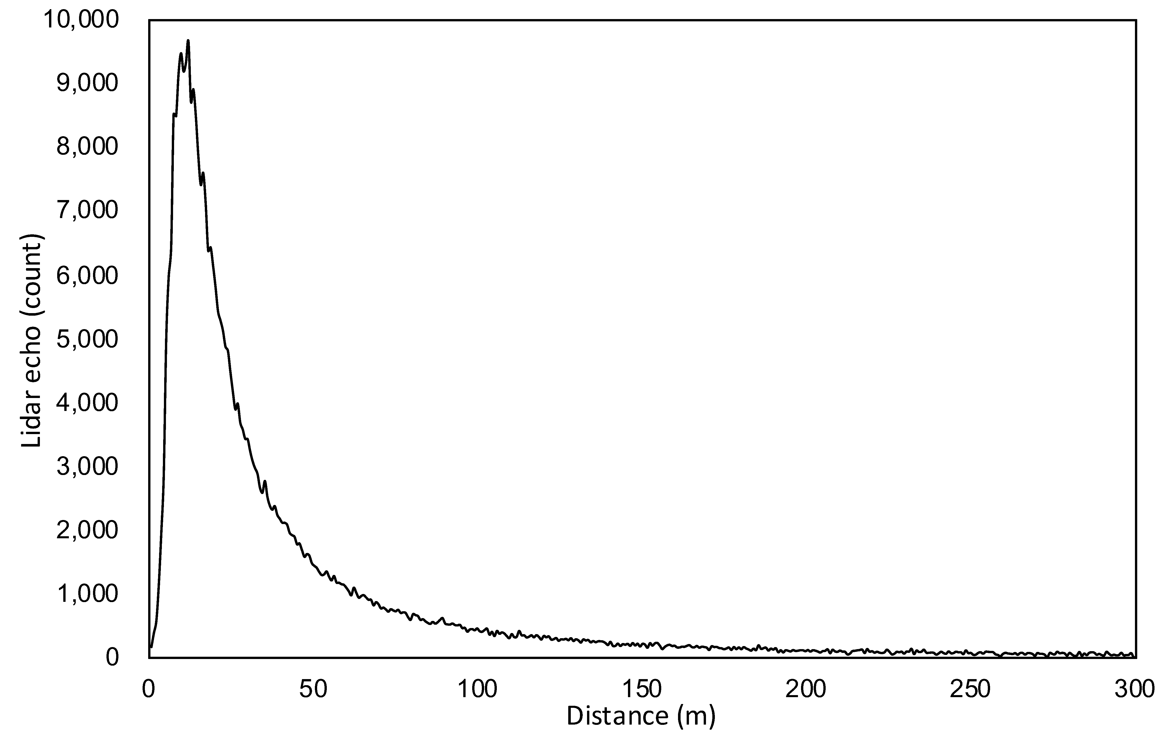
3.2. Lidar Echo Signal and Signal Processing

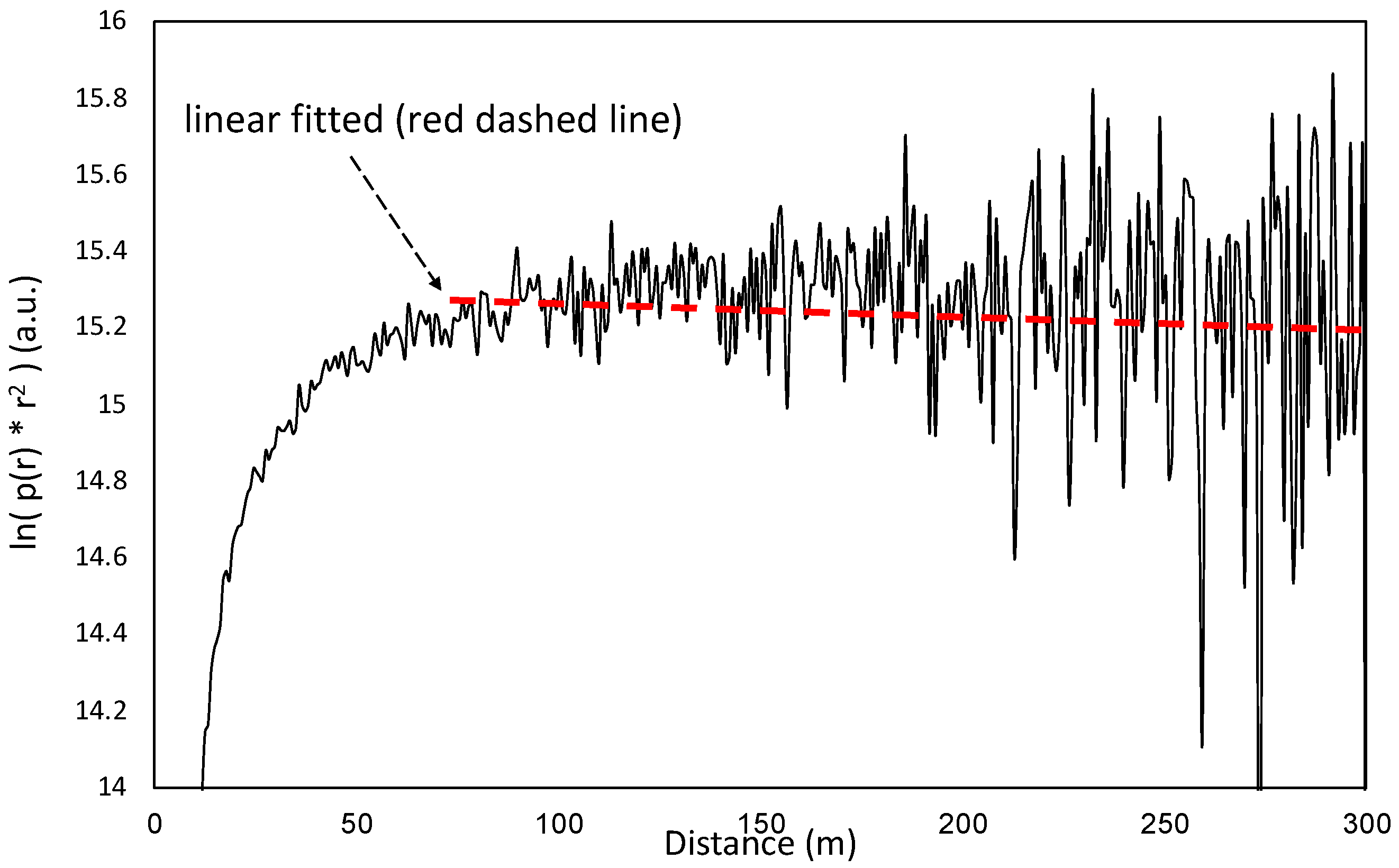
The analysis of LED-lidar echo signal is based on the lidar equation [24]:

$$P\left(r\right)=P_0·K·Y\left(r\right)·A_r·\frac{c\tau }{2}·\beta \left(r\right)·\frac{1}{r^2}·\exp \left(2\sigma r\right)$$

(11)

where $r$ is the measurement distance; $P\left(r\right)$ is the received power; $P_0$ is the transmitted power; $K$ is the system efficiency determined by the optical system of LED-lidar; $Y$ is the geometric overlap coefficient, representing the overlap rate of the field of view between receiver and transmitter, which is determined by the angle of view of transmitter and receiver; $A_r$ is the receiving area of the receiver determined by the aperture of the telescope; $c$ is the speed of light; $\tau$ is the pulse width of light; $\beta$ is the atmospheric backscattering coefficient; and $\sigma$ is atmospheric extinction coefficient.

Figure 3 shows the backscattering echo signals from atmospheric aerosols obtained by LED-lidar. The x-axis is the distance derived from the flight time of the photon. The y-axis is the intensity of the LED-lidar echo signal with the unit of count. At a distance of about 17 m, the geometric overlap coefficient of the system approaches 1, and the echo signal of atmospheric aerosol decreases exponentially with the increase in distance. As the geometric overlap coefficient increases gradually from 0 in the near distance, the backscattering echo shows an increasing trend in the close space. The maximum signal in the waveform is the point where the field overlap rate of the transmitter and receiver reaches the top. The geometric overlap coefficient reaches the top. Only the part of the signal farther than the maximum point can effectively evaluate the optical properties of atmospheric aerosol. The echo signal contains harmonic noise carried from the pulse modulation process. Due to the short pulse width of 10 ns and the precision of the modulation circuit, it is easy to form unstable harmonics, which become a part of the echo noise after being amplified by the LED driver. The background light is another kind of echo noise. Especially for the echo with low intensity obtained from a far distance, it is more susceptible to the influence of background light.

Atmospheric extinction coefficient $\sigma$ is an important parameter used to evaluate the optical characteristics of atmospheric aerosol. Although the atmospheric extinction coefficient has a spatial distribution, it is difficult to find the reference of the spatial distribution of the extinction coefficient on the surface to evaluate the denoising effect. Therefore, the average atmospheric extinction coefficient within a period of time is used as a reference to evaluate the denoising effect. The most classical slope method [25] is adopted to derive the parameter $\sigma$. The deriving process of $\sigma$ is as follows:

(a)

Carrying out the product operation of r² for both sides of the lidar equation.

(b)

Taking the natural logarithm for both sides of the equation.

(c)

Taking the derivative of r for both sides of the equation.

As the parameters $P_0$, $K$, $Y\left(r\right)$, $A_r$, $c$, and $\tau$ are constant, the new equation can be written as:

$$\frac{d\ln \left(P\left(r\right)·r^2\right)}{dr}=\frac{1}{\beta \left(r\right)}·\frac{d\beta \left(r\right)}{dr}-2\sigma$$

(12)

Considering that the atmosphere is homogeneous, and the backscattering coefficient $\beta$ is a constant, then $d\beta \left(r\right)/dr=0$. The homogeneous atmospheric extinction coefficient can be expressed in the following form:

$${\sigma }_0\left(r\right)=\frac{1}{2}·\frac{d\ln \left(P\left(r\right)·r^2\right)}{dr}$$

(13)

According to Equation (12), compensating the echo signal by multiplication of $r^2$, and taking the natural logarithm, the extinction coefficient can be derived as 1/2 of the slope of the compensated waveform, which is formed by the function of $\ln \left(P\left(r\right)·r^2\right)$.

Figure 4 shows the waveform of the LED-lidar echo after range compensation. Due to the low signal intensity of the long-range echo, the compensated echo signal is easily affected by the background light noise. After the range compensation, the background light noise at the long range is further amplified, making the signal at the long range unstable. The slope of the middle and rear waveform is calculated as the extinction coefficient. The red dashed line is a linear fitted line obtained from the part of the range compensation signal, which is further than 100 m, and 1/2 of its slope is the extinction coefficient characterized by the LED-lidar. The instability of the signal at the long range is prone to error in the process of the linear fit, especially when batch processing large amounts of LED-lidar echo data. Therefore, for the high-accuracy linear fit of the range compensation signal, effective LED-lidar echo denoising is an indispensable work in this study.

4. Result

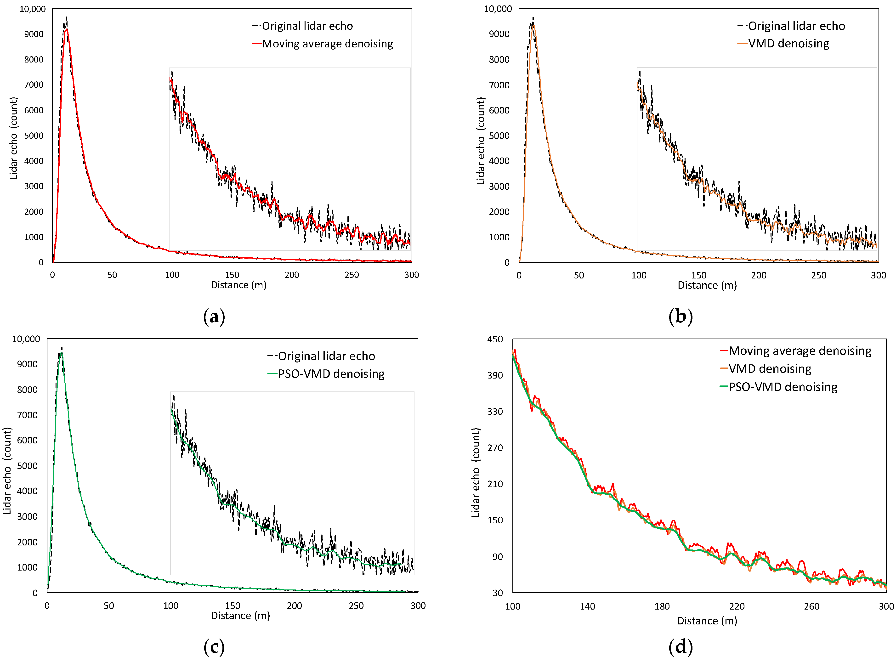
4.1. Denoising of LED-Lidar Echo

The moving average, VMD, and PSO-VMD are used to denoise the atmospheric aerosol echo signals of the LED-lidar. The denoising results are shown in Figure 5. Figure 5a–c shows the denoising results using moving average, VMD, and PSO-VMD, respectively, and the details of the waveform in the interval from 100 m to 300 m are shown in the box on the right side of the figure. Figure 5d shows the comparison of the denoising effect of the three methods. In Figure 5a, the result of the denoised echo is based on the 5-point moving average, which shows that the moving average method can effectively suppress the noise and make the echo signal smooth partly. The longer the moving average length, the better the noise suppression effect. However, the information is easily lost if the average length is set as a large value. Due to the steep gradient of signal intensity in the peak region, part of the information in the peak region is lost after moving average denoising, which is the disadvantage of the moving average method. Figure 5b shows the denoising results of the VMD with the empirical parameters [α = 200, K = 5]. The selection of parameters [α, K] is crucial in VMD denoising. For the same set of data, different parameter selection can achieve other denoising effects. Similarly, for the same set of empirical parameters [α, K], different denoising effects can be obtained when processing other data. Compared with the moving average method, the VMD method not only overcomes the disadvantage of the information loss brought by the moving average method due to a long moving average but also better suppresses the signal fluctuations in the region of low intensity. Figure 5c shows the denoising results based on PSO-VMD. As the initialization of PSO, the article swarm size is set as 10, maximum iterations number is set as 10, and minimum fitness value is set as 0.001. Thanks to the parameter optimization of PSO, the denoised echo signal not only maintains the same intensity level as the original echo signal but also finely rejects the subtle noise. The denoised echo signal is smoother than the one obtained by the empirical parameters of VMD. Figure 5d shows the comparison of the three methods of denoising results in the region of 100–300 m. The moving average denoising not only has information loss but also cannot suppress the signal fluctuation caused by the noise. The PSO-VMD has the best performance in signal denoising and fluctuation suppressing.

In the measurement of atmospheric aerosols, the ideal lidar echo should be close to the exponential attenuation when the distribution of aerosols is uniform, and the geometric overlap coefficient of the lidar system is 1. Fifty samples are selected from the denoising signals obtained by the three different methods and the original echo signal, respectively. The 100–300 m range of the signal was selected and fitted exponentially. The average R-square and root mean squared error (RMSE) were calculated. The calculation results are shown in

Table 1. Comparison of R-square and RMSE with the three denoising methods.

Denoising Method	R-Square	RMSE
Original echo	0.9421	24.0928
Moving average	0.9902	9.7450
VMD	0.9945	7.3588
PSO-VMD	0.9972	5.7369

The R-square represents the similarity between the experimental signal and the ideal fitted signal. The closer the value is to 1, the closer the experimental signal is to the ideal fitted signal. Compared with the original echo signal before denoising, the R-square values of the denoised signals are significantly improved, especially for the PSO-VMD denoising, the R-square value reaches the highest value of 0.9972. RMSE represents the deviation between the experimental signal and the ideal fitted signal. The smaller the value is, the closer the experimental signal is to the ideal fitted signal. Compared with the original signal before denoising, the RMSE of the signal after denoising decreased significantly, especially the RMSE of the PSO-VMD denoising result, which reaches the minimum value of 5.7369. Although the optimization parameters based on experience were used in VMD denoising, due to the difference between signals caused by the random error of measurement environment and background light, it is difficult to achieve the optimal denoising of all data with the optimization parameters based on experience. Comparing the R-Square and RMSE values of VMD and PSO-VMD, it shows that PSO has a significant optimization effect on VMD in LED-lidar denoising.

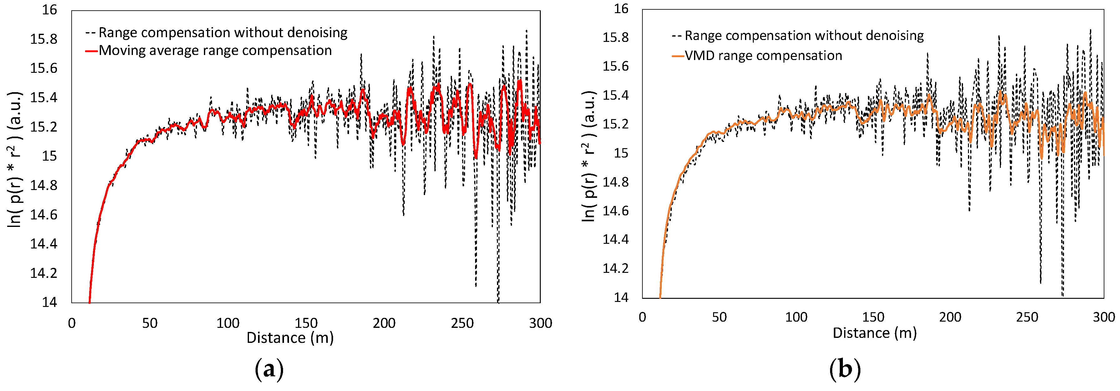
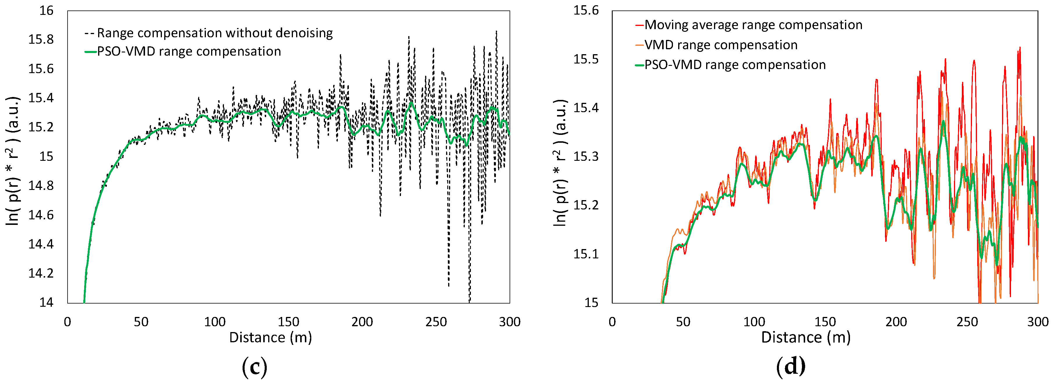
4.2. Range Compensation

As mentioned in Section 3.2, before solving the extinction coefficient of the LED-lidar aerosol echo signal with the slope method, the range compensation is required. However, as the distance increases, the compensated value to the echo signal gradually increases, and the noise is also amplified by the multiplication of range compensation. The signal-to-noise ratio of the distant echo signal is smaller than that of the near echo signal, which leads to increasing fluctuations in the range compensation as the distance increases. The fluctuation of the range compensation brings a significant error to calculating the slope by a linear fit. The range compensation was carried out after denoising the original echo signal of LED-lidar by moving average, VMD, and PSO-VMD, respectively. The calculation results are shown in Figure 6. Figure 6a–c show the range compensation results by using the denoised signal to deal with the moving average method, VMD, and PSO-VMD, respectively. Comparing the range compensation results of the echo signal after denoising by the three methods with that of the original signal, the fluctuation of the distant signal is suppressed. The denoising process removes part of the noise in the distant signal with low SNR, which reduces the noise amplification from the range compensation. Figure 6d compares the range compensation results denoised by the three methods. Compared with the moving average method, the range compensation result of VMD denoising has some improvement in suppressing fluctuation. However, the effect is not apparent, since IMF components K determined empirically is not the optimal value. On the other hand, compared with the VMD denoising, the PSO-VMD denoised range compensated signal is significantly improved in signal fluctuation. The high-frequency components from background noise and white noise are also suppressed, which is the effect of the critical parameters of K and α optimized by the PSO.

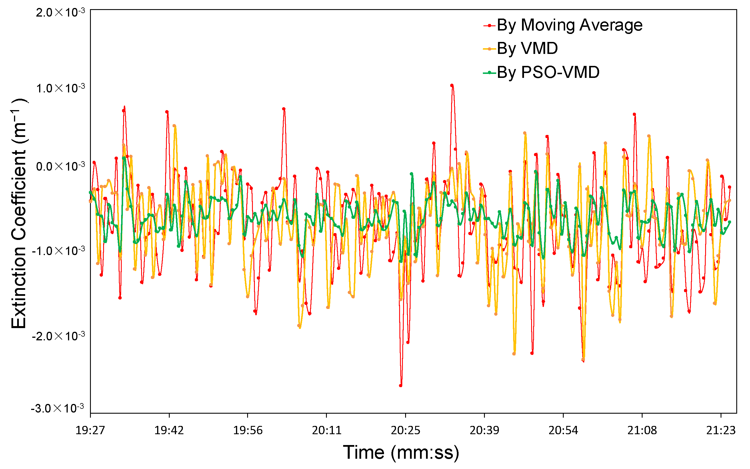
4.3. Extinction Coefficient

A set of LED-lidar echoes containing 196 samples was denoised with moving average, VMD, and PSO-VMD, and the extinction coefficients at different time points were derived. The samples were acquired on the night of 26 March 2019 (cloudy) in the city of Changde. The LED-lidar was set on the 6th floor of the second laboratory building of the Hunan University of Arts and Sciences, with an elevation angle of 60°. The period of sample acquisition was from 19:27 to 21:24. The number of data integration times was set as 10⁵ (mentioned in Section 3.1), and the acquisition time of each sample was about 40 s.

Figure 7 shows the extinction coefficients derived from the data in the region of 100–300 m, which was denoised by the moving average, VMD, and PSO-VMD. For all the samples, the PSO initialization was set as the parameters mentioned in Section 4.1. The x-axis is the time point, and the y-axis is the extinction coefficient. Although the calculation region and the elevation angle of LED-lidar were set as constant, the extinction coefficients derived by three methods fluctuated by varying degrees. The instability of the extinction coefficient is influenced by the flow of surface–atmosphere and variations of surface urban environmental conditions. On the other hand, the nonlinear signal itself, the influence of noise, and the poor adaptability of the fitting algorithm are also the reasons causing the extinction coefficients to fluctuate. According to Lambert Beer’s law, the extinction coefficient, in theory, should be negative values because of the light scattering in the atmosphere when light propagates in the atmosphere. However, some extinction coefficients with positive values were still obtained in this study. Due to the intense background light appearing in some data samples, even the excellent PSO-VMD method could not remove the noise at a long distance, which leads to the fact that as the noise is amplified in the process of range compensation, the range compensated signal intensity at a long distance is higher than that at a short distance. The slope of the linear fitting becomes a positive value. Compared with the derived extinction coefficients by moving average and VMD method, the number of positive values of extinction coefficients derived by the PSO-VMD method is only 4, which is the least. The result indicates that the PSO-VMD method can remove the noise from background light more effectively. The standard deviations of the extinction coefficients derived by moving average, VMD, and PSO-VMD were calculated, and the values were 5.7452 × 10⁻⁴, 4.7309 × 10⁻⁴, and 2.2896 × 10⁻⁴, respectively. Due to the superiority of PSO-VMD denoising, the fluctuation of extinction coefficients obtained by PSO-VMD is minimal.

To evaluate the accuracy of the extinction coefficients derived from the LED-lidar echo, the extinction coefficients were derived from the surface visibility released by the Hunan provincial meteorological department and compared with the average values of the three sets of extinction coefficients calculated from LED-lidar echo. The conversion formula from visibility to extinction coefficient is expressed as Equation (14):

$$\sigma =\frac{3.912}{\nu }·\frac{550}{\lambda }$$

(14)

where $\sigma$ is the extinction coefficient, $\nu$ is the visibility, and $\lambda$ is the wavelength of the light source. The visibility on March 26 was about 10 km, and the wavelength of the light source was 395 nm. According to the parameters of visibility and wavelength, the extinction coefficient was calculated as 5.6 × 10⁻⁴ m⁻¹. The mean values of extinction coefficients derived by moving average, VMD, and PSO-VMD were 6.7609 × 10⁻⁴ m⁻¹, 6.4250 × 10⁻⁴ m⁻¹, 5.7401 × 10⁻⁴ m⁻¹, respectively. The average value of the extinction coefficient derived by PSO-VMD is closest to the value of the extinction coefficient derived from visibility, which indicates the superiority of PSO-VMD in extinction coefficient calculation.

5. Conclusions

For the characteristics of nonlinear, low SNR, and low dynamic range in LED-lidar echo signal, a novel denoising method based on VMD with adaptive-weight PSO is proposed. Compared with the traditional VMD denoising method, this method dynamically assigns the weights $\omega$ in the PSO algorithm for the different echo signals. It globally optimizes the critical parameters [α, K] of VMD, which further improves the denoising effect.

Echo signal denoising, range compensation, and extinction coefficient calculation were performed by using moving average, VMD, and PSO-VMD, respectively. The denoised echo signal based on PSO-VMD has the optimal R-square value of 0.9972 and the minimum RMSE value of 5.7369. In the calculation of range compensation, the result based on PSO-VMD denoising has the slightest fluctuation at long distance. In the analysis of extinction coefficient, the extinction coefficients based on PSO-VMD denoising have the best stability. Under the condition of intense background light and incomplete denoising, the number of error points of slope fitting with PSO-VMD denoising is the least. The superiority of PSO-VMD in LED-lidar denoising is proved by analysis of the three critical signals.

However, a constant region and parameters were used in the calculation of linear fitting, resulting in a small number of slope fitting error points when the SNR of the echo signal is low and the fluctuation is significant. In the future, the introduction of machine learning is considered, which can better perform adaptive linear fitting to further reduce the fluctuation of extinction coefficient.

References

1. Jaboyedoff, M.; Oppikofer, T.; Abellán, A.; Derron, M.; Loye, A.; Metzger, R.; Pedrazzini, A. Use of lidar in landslide investigations: A review. Nat. Hazards 2012, 61, 5–28. [Google Scholar] [CrossRef] [Green Version]
2. Qiu, J.; Lu, D. On lidar application for remote sensing of the atmosphere. Adv. Atmos. Sci. 1991, 8, 369–378. [Google Scholar]
3. Thayer, J.P. Rayleigh lidar system for middle atmosphere research in the arctic. Opt. Eng. 1997, 36, 2045–2061. [Google Scholar] [CrossRef]
4. Carswell, A.I.; Pal, S.R.; Steinbrecht, W.; Whiteway, J.A.; Ulitsky, A.; Wang, T.Y. Lidar measurements of the middle atmosphere. Can. J. Phys. 1991, 69, 1076–1086. [Google Scholar] [CrossRef]
5. Nishizawa, T.; Jin, Y.; Sugimoto, N.; Sato, K.; Okamoto, H. Observation of clouds, aerosols, and precipitation by multiple-field-of-view multiple-scattering polarization lidar at 355 nm. J. Quant. Spectrosc. Radiat. Transf. 2021, 271, 107710. [Google Scholar] [CrossRef]
6. Ninomiya, H.; Yaeshima, S.; Ichikawa, K.; Fukuchi, T. Raman lidar system for hydrogen gas detection. Opt. Eng. 2007, 46, 094301. [Google Scholar] [CrossRef]
7. Choi, I.Y.; Baik, S.H.; Cha, J.H.; Kim, J.H. Hydrogen gas concentration measurement method using the raman lidar system. Meas. Sci. Technol. 2019, 30, 055201. [Google Scholar] [CrossRef]
8. Zeyn, J.; Lahmann, W.; Weitkamp, C. Remote daytime measurements of tropospheric temperature profiles with a rotational raman lidar. Opt. Lett. 1996, 21, 1301–1303. [Google Scholar] [CrossRef]
9. Chust, G.; Galparsoro, I.; Ángel, B.; Franco, J.; Uriarte, A. Coastal and estuarine habitat mapping, using lidar height and intensity and multi-spectral imagery. Estuar. Coast. Shelf Sci. 2008, 78, 633–643. [Google Scholar] [CrossRef]
10. Lin, Y.; Hyyppa, J.; Jaakkola, A. Mini-uav-borne lidar for fine-scale mapping. IEEE Geosci. Remote Sens. Lett. 2011, 8, 426–430. [Google Scholar] [CrossRef]
11. Fisher, C.T.; Cohen, A.S.; Fernández-Diaz, J.C.; Leisz, S.J. The application of airborne mapping lidar for the documentation of ancient cities and regions in tropical regions. Quatern. Int. 2017, 448, 129–138. [Google Scholar] [CrossRef]
12. Koyama, M.; Shiina, T. Light source module for led mini-lidar. Rev. Laser Eng. 2011, 39, 617–621. [Google Scholar] [CrossRef] [Green Version]
13. Shiina, T. LED mini lidar for atmospheric application. Sensors 2019, 19, 569. [Google Scholar] [CrossRef] [Green Version]
14. Rocadenbosch, F.; Soriano, C.; Comerón, A.; Baldasano, J.M. Lidar inversion of atmospheric backscatter and extinction-to-backscatter ratios by use of a Kalman filter. Appl. Opt. 1999, 38, 3175–3189. [Google Scholar] [CrossRef] [Green Version]
15. Zhou, Z.; Hua, D.; Wang, Y.; Yan, Q.; Li, S.; Yan, L.; Wang, H. Improvement of the signal to noise ratio of Lidar echo signal based on wavelet de-noising technique. Opt. Laser Eng. 2013, 51, 961–966. [Google Scholar] [CrossRef]
16. Yang, G.; Liu, Y.; Wang, Y.; Zhu, Z. EMD interval thresholding denoising based on similarity measure to select relevant modes. Signal Process. 2015, 109, 95–109. [Google Scholar] [CrossRef]
17. Yan, S.; Yang, G.; Li, Q.; Wang, C. Waveform centroid discrimination of pulsed Lidar by combining EMD and intensity weighted method under low SNR conditions. Infrared Phys. Technol. 2020, 109, 103385. [Google Scholar] [CrossRef]
18. Dragomiretskiy, K.; Zosso, D. Variational mode decomposition. IEEE Trans. Signal Process. 2013, 62, 531–544. [Google Scholar] [CrossRef]
19. Li, J.; Zhang, X.; Tang, J. Noise suppression for magnetotelluric using variational mode decomposition and detrended fluctuation analysis. J. Appl. Geophys. 2020, 180, 104127. [Google Scholar] [CrossRef]
20. Liu, Z.; Chang, J.; Li, H.; Chen, S. Signal denoising method combined with variational mode decomposition, machine learning online optimization and the interval thresholding technique. IEEE Access 2020, 8, 223482–223494. [Google Scholar] [CrossRef]
21. Diao, X.; Jiang, J.; Shen, G.; Chi, Z.; Wang, Z.; Ni, L.; Mebarki, A.; Bian, H.; Hao, Y. An improved variational mode decomposition method based on particle swarm optimization for leak detection of liquid pipelines. Mech. Syst. Signal Pract. 2020, 143, 106787. [Google Scholar] [CrossRef]
22. Garg, H. A hybrid PSO-GA algorithm for constrained optimization problems. Appl. Math. Comput. 2016, 274, 292–305. [Google Scholar] [CrossRef]
23. Behnam, M.; Pourghassem, H. Spectral correlation power-based seizure detection using statistical multi-level dimensionality reduction and PSO-PNN optimization algorithm. IETE J. Res. 2017, 63, 736–753. [Google Scholar] [CrossRef]
24. Eloranta, E.E. High Spectral Resolution Lidar. In Springer Series in Optical Sciences; Georgia Institute of Technology: Atlanta, GA, USA, 2005; Volume 102, pp. 143–163. [Google Scholar]
25. Kunz, G.J.; Leeuw, G. Inversion of lidar signals with the slope method. Appl. Opt. 1993, 32, 3249–3256. [Google Scholar] [CrossRef] [PubMed]
Figure 1. Flowchart of the adaptive-weight particle swarm optimization (PSO) - variational modal decomposition (VMD).
Information 13 00558 g001
Figure 2. LED-lidar system: (a) schematic diagram; (b) prototype.
Information 13 00558 g002
Figure 3. A typical backscattering echo signals from atmospheric aerosols.
Information 13 00558 g003
Figure 4. LED-lidar echo waveform after range compensation.
Information 13 00558 g004
Figure 5. Denoising result of LED-lidar echo: (a) moving average; (b) VMD; (c) PSO-VMD; (d) comparison of (ac).
Information 13 00558 g005
Figure 6. LED-lidar echo range compensation: (a) moving average; (b) VMD; (c) PSO-VMD; (d) comparison of (ac).
Information 13 00558 g006aInformation 13 00558 g006b
Figure 7. The extinction coefficients of atmospheric aerosol derived by three denoising methods.
Information 13 00558 g007