A Bottleneck Auto-Encoder for F0 Transformations on Speech and Singing Voice

Abstract

In this publication, we present a deep learning-based method to transform the $f_0$ in speech and singing voice recordings. $f_0$ transformation is performed by training an auto-encoder on the voice signal’s mel-spectrogram and conditioning the auto-encoder on the $f_0$. Inspired by AutoVC/F0, we apply an information bottleneck to it to disentangle the $f_0$ from its latent code. The resulting model successfully applies the desired $f_0$ to the input mel-spectrograms and adapts the speaker identity when necessary, e.g., if the requested $f_0$ falls out of the range of the source speaker/singer. Using the mean $f_0$ error in the transformed mel-spectrograms, we define a disentanglement measure and perform a study over the required bottleneck size. The study reveals that to remove the $f_0$ from the auto-encoder’s latent code, the bottleneck size should be smaller than four for singing and smaller than nine for speech. Through a perceptive test, we compare the audio quality of the proposed auto-encoder to $f_0$ transformations obtained with a classical vocoder. The perceptive test confirms that the audio quality is better for the auto-encoder than for the classical vocoder. Finally, a visual analysis of the latent code for the two-dimensional case is carried out. We observe that the auto-encoder encodes phonemes as repeated discontinuous temporal gestures within the latent code.

1. Introduction

Since the invention of the vocoder over 80 years ago [1], people have been studying means to transform the acoustical properties of speech recordings. Since then, enabling transparent $f_0$ transformations has been a prominent topic inside the speech processing research community, and attempts to achieve this have been plentiful, such as the phase vocoder [2], PSOLA [3], shape-invariant additive models [4], shape-invariant phase vocoder [5], parametric speech vocoders [6,7], and extended source-filter models [8,9]. Recently, as speech signal processing has become dominated by deep learning-based techniques, the community has focused on more abstract voice properties, such as speaker identity [10,11,12,13,14,15] but also emotion [16,17] and accent [18].

Transforming the $f_0$ of the singing voice is crucial for singing synthesis and could also help refine existing recordings. In the singing voice, the $f_0$ not only carries the melody, but also the singer’s individual expression used to interpret the piece, which is highly dependent on the genre of the piece [19]. Therefore, for singing synthesis, it does not suffice to simply map the notes to their corresponding frequencies and durations. Singing synthesizers need to translate the required melody to an $f_0$ curve to convey the expression and style required by the score [20,21]. A common approach is unit selection with $f_0$ modification [22,23]. The quality of these synthesizers is thus limited by the quality of the transposition algorithm. Combining singing units in mel-spectrum representation with the neural $f_0$ transformation introduced in this paper, along with our mel-inverter described in [24], could allow creating a fully neural singing synthesizer. As for voice modification, $f_0$ transformation can also be used on real singing recordings to alter the intonation, expression and even melody in post production. The $f_0$ transformation algorithm presented here could also expand the range of a singer. If pushed far enough, thanks to the implicit adaptation of voice features, it will create a coherent new personality.

In speech, the $f_0$ plays a different role than in singing. It carries important information, such as mood, intent and identity. To change the expressivity of an utterance, we need to be able to change the $f_0$ contour [25]. One of the most prominent differences between the sexes is the mean $f_0$, due to the different rates of growth of the vocal folds in puberty. Thus, changing the $f_0$ in speech can result in changing or obfuscating the speaker’s gender [26], an effect which could be used in scientific studies to research the effect of perceived gender in the voice in social interactions [27].

1.1. Related Work

The simplest way to achieve an $f_0$ transformation effect is changing the playback speed of a signal. The most obvious side effect of this is that the durations change as well. To counter this, phase vocoders [2] reverse the change in duration with time stretching: they shift frames in time and adapt the phase accordingly. After the stretching, the signal is resampled appropriately. However, this technique shifts the fundamental frequency and its partials as well as their amplitudes, i.e., the whole spectral envelope is stretched in frequency. Since the spectral envelope reflects the size of the vocal tract, the result is the well-known Mickey Mouse effect, which hints at an unnatural vocal tract size. To prevent this, special treatment of the spectral envelope is required [5].

Another approach from classical signal processing is using a vocoder that has $f_0$ as one of its parameters [3,6,7]. In this case, the $f_0$ can be changed simply by providing the desired $f_0$ to the synthesizer of the vocoder. However, the $f_0$ of speech also has an effect on the remaining vocoder parameters, and thus a mismatch during synthesis is often perceived as being unnatural [28]. To address this problem, extended source filter models [8,9] split the spectral envelope into a vocal tract filter and the glottal pulse spectrum, while the $f_0$ dependency is modeled by a glottal pulse model. This works fine for small amounts of transpositions but still has its limitations, as relationships between the $f_0$ and the vocal tract are not considered.

Due to the inherent complexity of relationships between the $f_0$, glottal pulse and vocal tract filter, we believe that these effects can best be modeled with data-driven approaches. Deep learning-based attribute transformation has seen a few breakthroughs in image processing over the recent years and the literature has been rich on the topic. Style transfer was used to separate content and “style” to create effects that cast the visual appearance of famous paintings over photos [29]. Generative adversarial networks (GAN) [30] have been used in different configurations for attribute transformation [31], in particular, speaker identity conversion [12,15]. Auto-encoders [32] can be used to disentangle attributes from the auto-encoder’s latent code, either implicitly with an information bottleneck [14] or explicitly with an adversarial classifier on the latent code [33]. Auto-encoders have been applied to speech to disentangle the speaker identity [10,14] and even split speech into rhythm, pitch, timbre and content, simultaneously [34].

1.1.1. F0 Analysis

To be able to manipulate the $f_0$, we first need to be able to extract the $f_0$ from signals. $f_0$ estimation has many applications and a long history. Classical signal processing methods can be divided by the domain that they operate on, being either the cepstrum [35], the auto-correlation function [36,37] or the frequency domain [38]. These methods were developed to work on quasiperiodic signals in general, e.g., speech, music, and medical signals, and special adaptions to the singing voice have been made by [39,40]. Neural networks have been trained to extract the $f_0$ from speech and singing voices from raw audio [41,42] or mel-spectrograms [43]. In this paper, we use [42].

1.1.2. Voice Transformation on Mel-Spectrograms

Our proposed system allows changing the $f_0$ of a given recording of speech or a singing voice by transforming the signal’s mel-spectrogram. The transformed mel-spectrogram can then be converted back to raw audio by means of a mel-inversion algorithm.

Mel-spectrograms have become a common choice in text-to-speech applications [44,45] and voice conversion [13,14]. With fast and robust mel-inversion techniques [24,46], the mel-spectrogram is an attractive representation of human voice for deep learning-based approaches, as it organizes the relevant information in a compact and homogeneous fashion.

1.1.3. Auto-Encoders

To perform $f_0$ transformations, we train an auto-encoder conditioned on the $f_0$. An auto-encoder consists of an encoder–decoder pair of neural networks. The idea is that the encoder produces a latent code representing selected features of the input signal. The decoder receives the latent code and maps its input back to the original input space. The decoder can be conditioned on additional information, such as, in our case, the $f_0$. This introduces a redundancy between the latent code and the conditional input. To perform attribute transformation, one has to make sure that the decoder uses the attribute from the conditional input, rather than from the latent code. This can be achieved by removing the attribute in question entirely from the latent code, in which case we say that the attribute is disentangled from the latent code. If the decoder is conditioned with the original attribute value, it should reverse the encoder’s operation and reproduce the original signal exactly. If the attribute is successfully disentangled from the latent code, the decoder would then produce a plausible output with the provided attribute value regardless of the attribute value. The difficulty of an auto-encoder approach is the disentanglement—finding a way to force the decoder to use the provided attribute rather than inferring it from the latent code.

A simple but effective approach for disentanglement is through the use of an information bottleneck [14]. Typically in an auto-encoder setup, the latent code has a lower dimensionality than the input signal. Theoretically, the domains of the signal and the latent code have the same cardinality (all finite-dimensional $\mathbb{R}$-vector spaces have uncountable many elements), and thus, there are bijective mappings between them. In practice, however, the modeling capacity of the neural networks is limited, and thus, the space of the latent code has less channel capacity than the space of the original signal. Some information is, thus, removed during the encoding process. When training the auto-encoder on auto-reconstruction, the encoder will learn to prioritize information that is important for recreating the original signal. Since the attribute is provided to the decoder in the conditional input, there is no benefit in providing it again to the decoder through the latent code. Consequently, if the information bottleneck is small enough, the encoder can be expected to first remove the redundant attribute from the latent code.

1.2. Contributions

The novelties of this paper are the following. (1) We propose the first deep learning-based algorithm, explicitly focusing on the $f_0$ transformation of singing and speaking voices, using the absolute $f_0$. The proposed system is able to accurately follow the desired $f_0$ within the typical ranges of the human voice and even outside the range of the source speaker, while surpassing the audio quality of classical vocoders. These claims are supported by analyzing the $f_0$ error on the test set in Section 3.1 and by a perceptive test, which we present in Section 3.3. Since the proposed system uses an auto-encoder with information bottleneck [14], we (2) perform a thorough study on how disentanglement depends on the bottleneck size, the size of the neural network, the dataset size and the voice type (speech vs. singing voice). The results of this analysis are given in Section 3.1. (3) Finally, we carry out a visual analysis on the latent code of the auto-encoder, where we find the phonetic content to be represented as periodic discontinuous patterns by the auto-encoder.

The remainder of the paper is structured as follows. In Section 2, we formulate the central question of this paper, introduce the auto-encoder setup, its architecture and how to train it, the datasets used in the experiments and the experimental setup itself. In Section 3, we present the results from a perceptive test and a transformation accuracy analysis, where we compare the proposed system to other $f_0$ transformation algorithms, as well as a visual analysis of the latent code for the case where the bottleneck size is two. The conclusion and outlook for future work can be found in Section 4.

2. Materials and Methods

2.1. Problem Formulation

The problem we try to solve in this study is the free modification of the fundamental frequency $f_0$ in recordings of speech and singing voices. The algorithm should require only minimal input from the user and should allow one to change the $f_0$ by providing a fixed transposition value or redrawing the $f_0$ curve.

Unlike [34], where the pitch is defined as the part of the speech melody that is independent from rhythm, timbre and content, in this paper, we use the raw $f_0$ as the control parameter. Therefore, the control parameter for our auto-encoder contains some information about the speaker’s identity and timbre. Changing the raw $f_0$ signal may change the component of the speaker identity and timbre that depends on the $f_0$. The system should apply the given $f_0$ contour onto the output signal such that the output signal contains exactly the same $f_0$ contour. This implies that parts of the identity will change if the change is incompatible with the speaker ID.

Two main goals arise for a potential $f_0$ transformation system:

• The desired $f_0$ contour should be followed exactly;
• The result should sound like a human.

The first goal, the $f_0$ accuracy, can be evaluated objectively by resynthesizing the transformed mel-spectrograms and checking that the $f_0$ in the resynthesized audio matches the target $f_0$. Our findings are stated in Section 3.1. The second objective, the naturalness of the syntheses, can only be evaluated by listening to the generated samples. Therefore, we perform a perceptive study by asking a selected group of participants to listen to synthesized and non-synthesized audio and give a perceptive rating. The results of the perceptive test are presented in Section 3.3.

To perform the $f_0$ transformation, we train an auto-encoder with an information bottleneck [14] as described in Section 1.1.3. One crucial hyperparameter of such a model is the size of the bottleneck. We, therefore, perform a systematic analysis of the dependence between the disentanglement and bottleneck size, and present the results in Section 3.2.

2.2. Proposed Model

The general outline of the proposed system can be seen in Figure 1. The auto-encoder in this paper operates on mel-spectrograms. To change the $f_0$, we first extract the mel-spectrogram and the $f_0$ from the original audio recording. Then, we use the encoder to produce a latent code from the mel-spectrogram and the original $f_0$. We resynthesize the mel-spectrogram by applying the decoder to the latent code and the target $f_0$. Finally, the transformed audio is obtained by inverting the transformed mel-spectrogram using the neural vocoder we presented in [43].

2.2.1. Input Data

The mel-spectrograms are computed on $24\mathrm{kHz}$ audio. We use 80 mel-bands to represent the frequencies between 0 and $8\mathrm{kHz}$. Frequencies above $8\mathrm{kHz}$ are disregarded and expected to be completed coherently by the final mel-inverter. The mel-spectrograms have a hop size of $12.5\mathrm{ms}$, resulting in a 80-dimensional signal with an $80\mathrm{Hz}$ sample rate. The mel-spectrograms are given with logarithmic amplitudes. The $f_0$ curve is provided as a number pair $(log\left(f_0\right),\mathrm{voiced}/\mathrm{unvoiced}\mathrm{mask})$, and is generated from the audio signal by our $f_0$ analysis algorithm, F0-FCN [42].

To obtain normalized input data, we rescale the input data such that the interval $[-1,1]$ represents $[-120\mathrm{dB},-20\mathrm{dB}]$ for the mel-spectrograms and $[45\mathrm{Hz},1400\mathrm{Hz}]$ for the fundamental frequency $f_0$.

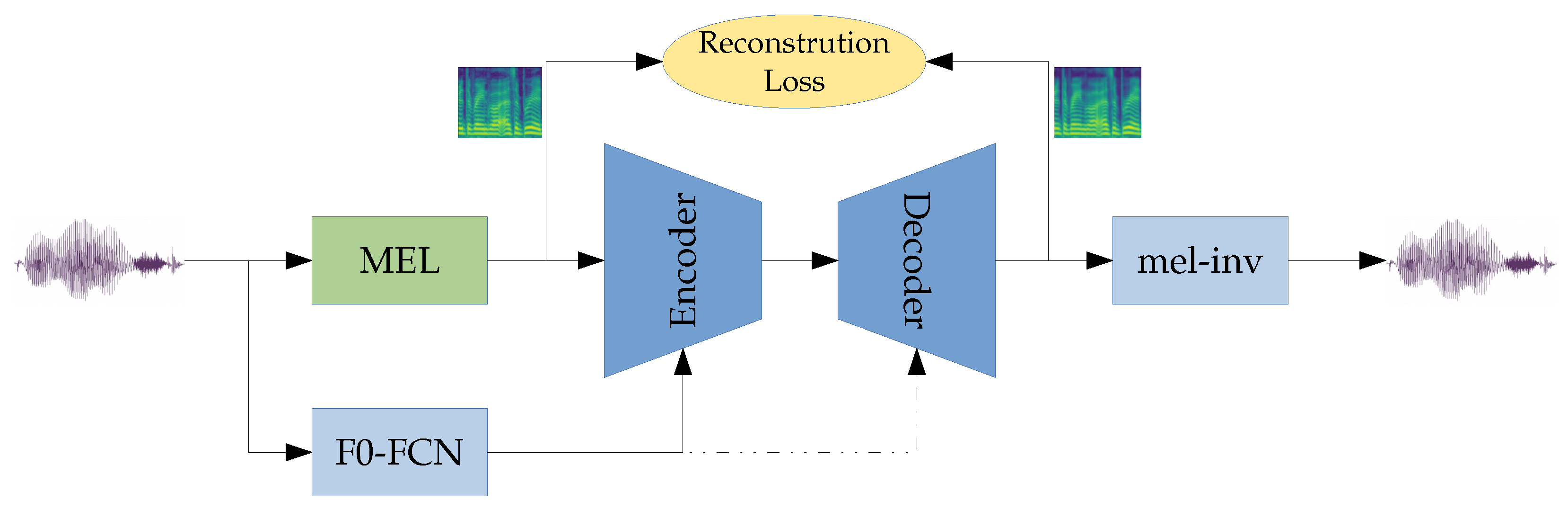
2.2.2. Network Architecture

The auto-encoder is implemented as a fully convolutional neural network, where the encoder and decoder resemble mirrored structures. To benefit from the natural topology of the frequency axis, we treat the sequence of mel-spectrograms as images and perform 2D convolutions on them [47]. Through strides in frequency direction, the encoder reduces the frequency axis to length 1 but keeps the time axis unchanged. The decoder uses transposed convolutions to incrementally rebuild the frequency axis. The exact architecture is provided in Appendix A (

Table A1. List of layers in the encoder.

Layer	Inputs	Output	#Filters	Kernel Size	Stride	Activation	Out Shape
Conv2DTranspose	$f_0$	$f_0^{\prime }$	2	(1, 80)	$(1,80)$	none	$(t,80,2)$
Concat	mel, $f_0^{\prime }$	$h_0$					$(t,80,3)$
Conv2D	$h_0$	$h_1$	512	$(1,2)$	$(1,2)$	ReLU	$(t,40,512)$
Conv2D	$h_1$	$h_2$	512	$(3,3)$		ReLU	$(t,40,512)$
Conv2D	$h_2$	$h_3$	512	$(1,2)$	$(1,2)$	ReLU	$(t,20,512)$
Conv2D	$h_3$	$h_4$	512	$(3,3)$		ReLU	$(t,20,512)$
Conv2D	$h_4$	$h_5$	512	$(1,2)$	$(1,2)$	ReLU	$(t,10,512)$
Conv2D	$h_5$	$h_6$	512	$(3,3)$		ReLU	$(t,10,512)$
Conv2D	$h_6$	$h_7$	512	$(1,2)$	$(1,2)$	ReLU	$(t,5,512)$
Conv2D	$h_7$	$h_8$	512	$(3,3)$		ReLU	$(t,5,512)$
Conv2D	$h_8$	$h_9$	512	$(1,5)$	$(1,5)$	ReLU	$(t,1,512)$
Conv2D	$h_9$	code	$n_b$	$(3,1)$		none	$(t,1,n_b)$

and

Table A2. List of layers in the decoder.

Layer	Inputs	Output	#Filters	Kernel Size	Stride	Activation	Out Shape
Concat	code, $f_0$	$h_0^{\prime }$					$(t,1,n_b+2)$
Conv2D	$h_0^{\prime }$	$h_1^{\prime }$	512	$(3,3)$		ReLU	$(t,1,512)$
Conv2DTranspose	$h_1^{\prime }$	$h_2^{\prime }$	512	$(1,5)$	$(1,5)$	ReLU	$(t,5,512)$
Conv2D	$h_2^{\prime }$	$h_3^{\prime }$	512	$(3,3)$		ReLU	$(t,5,512)$
Conv2DTranspose	$h_3^{\prime }$	$h_4^{\prime }$	512	$(1,2)$	$(1,2)$	ReLU	$(t,10,512)$
Conv2D	$h_4^{\prime }$	$h_5^{\prime }$	512	$(3,3)$		ReLU	$(t,10,512)$
Conv2DTranspose	$h_5^{\prime }$	$h_6^{\prime }$	512	$(1,2)$	$(1,2)$	ReLU	$(t,20,512)$
Conv2D	$h_6^{\prime }$	$h_7^{\prime }$	512	$(3,3)$		ReLU	$(t,20,512)$
Conv2DTranspose	$h_7^{\prime }$	$h_8^{\prime }$	512	$(1,2)$	$(1,2)$	ReLU	$(t,40,512)$
Conv2D	$h_8^{\prime }$	$h_9^{\prime }$	512	$(3,3)$		ReLU	$(t,40,512)$
Conv2DTranspose	$h_9^{\prime }$	$h_{10}^{\prime }$	512	$(1,2)$	$(1,2)$	ReLU	$(t,80,512)$
Conv2D	$h_{10}^{\prime }$	mel’	1	$(3,3)$		none	$(t,80,1)$

).

In the encoder, we start with an “image” with the structure $\mathtt{time}\times \mathtt{frequency}$. This is stacked with the $f_0$ signal, which is resampled and extended on the frequency axis to match the size of the mel-frequency axis with a trainable linear projection (cf. Table A1). We then reduce the size of the frequency axis step by step through down-sampling until it has a length of 1. Down-sampling is performed with strided convolutions across the frequency dimension, and the down-sampling operations are intercalated with classic $3\times 3$ convolutions. The last layer of the encoder, a $3\times 1$ convolution, maps the features to the desired bottleneck size.

The decoder has an inverse structure with respect to the encoder. We start with the concatenation of the latent code and the target $f_0$ curve and broaden the frequency axis step by step by up-sampling. Up-sampling is performed through transposed convolutions. The final convolution maps the number of features back to 1, recreating the shape of the input mel-spectrogram.

All convolutions use zero-padding to keep the shapes consistent. Activation functions are ReLU [48]. Encoder and decoder have 10 and 11 convolutional layers, respectively, where each layer has 512 filters. The models have roughly $12.5\mathrm{M}$ parameters each.

Contrary to AutoVC [14], there is no temporal down-sampling in our approach. As AutoVC performs speaker identity conversion, the conditional input is constant in time. Thus, there, a precise temporal resolution is not important. Here, however, we condition on the $f_0$ signal, which varies over time, and aim to preserve the temporal structure implied by the $f_0$ signal as precisely as possible. Similarly, we use convolutional layers instead of RNN to focus the neural network to use more local features.

We also experimented with 1D convolutions but found the results’ quality to be inferior with respect to the 2D versions. We tried growing the number of features after each down-sampling of the frequency axis in the encoder, while equally decreasing the number of features in the decoder, but found no significant difference in the results when keeping the number of parameters and inference speed similar. Thus, we opted to keep the same number of features for each layer, regardless of the size of the frequency axis.

2.2.3. Training Procedure

The auto-encoder is trained only on self-reconstruction. We apply a point-wise mean absolute error loss between the input mel-spectrogram and the output of the decoder. Optimization is performed with ADAM [49], with a learning rate of $1\times {10}^{-4}$ and the parameters ${\beta }_1=0.9$ and ${\beta }_2=0.999$. We use a batch size of 16 training samples per batch with 80 time steps (equivalent to $1\mathrm{s}$) per sample. All models are trained for $250\mathrm{k}$ updates.

2.3. Datasets

In our experiments, we use the following four different datasets:

• A pure singing-voice dataset, obtained by combining several publicly available datasets and our own proprietary datasets;
• A pure speech dataset consisting of the English dataset VCTK [50] and the French dataset Att-HACK [51];
• A hybrid dataset of speech and singing, consisting of the two datasets above;
• A smaller speech dataset, consisting of a reduced number of VCTK speakers to match the duration of the singing-voice dataset.

In particular, the singing-voice dataset contains the following:

• CREL Research Database (SVDB) [52];
• NUS sung and spoken lyrics corpus [53];
• Byzantine singing from the i-Treasures Intangible Cultural Heritage dataset [54];
• PJS phoneme-balanced Japanese singing-voice corpus [55];
• JVS-MuSiC [56];
• Tohoku Kiritan and Itako singing database [57];
• VocalSet: A singing voice dataset [58];
• Singing recordings from our internal singing databases used for the IRCAM singing synthesizer [59] and other projects.

In total, the singing dataset contains $26.5\mathrm{h}$ of singing voices from 136 different singers; however, 100 of them are from JVS and 94% of the total duration is sung by the remaining 36 singers. Most of the singers in the dataset are professionals, but a few of them are also amateurs. For datasets which also contain speech, only the singing recordings are used. The dataset contains singing in English, French, Greek, Italian, Japanese and Latin.

For speech, we train on both VCTK [50] and Att-HACK [51] which amounts to a combined dataset of English and French speech, containing a total of 134 speakers (109 from VCTK, 25 from Att-HACK) and $54\mathrm{h}$ of speech ($32\mathrm{h}$ from VCTK, $22\mathrm{h}$ from Att-HACK).

To better compare the results between speech and singing voices, we also train models on a smaller speech dataset, consisting of only a subset of the VCTK speakers, resulting in $26.5\mathrm{h}$ of speech.

Dataset Splits

For evaluation, we withhold four speakers from the VCTK dataset in the following section: two female and two male speakers. These are p361, p362, p374 and p376. Thus, all evaluation of the speech models is performed on unseen speakers.

The test set for singing voices consists of five samples each from a set of different singers, aimed to include a representative of each voice class, including baritone, tenor, mezzo-soprano, soprano, child voice and counter tenor, and singing style, including classical, pop, J-pop and Byzantine singing.

2.4. Experimental Setup

The variety of sounds that can be produced with the human voice is rich, and the human voice is used in many different contexts. We usually make a distinction between speaking and singing voices, due to their different acoustic properties and applications. Similarly, here, we train separate models on speech and on singing. As speaking and singing have their differences, training a model only on one domain may improve its quality, as the difficulty of the task is reduced. On the other hand, speech and singing share many similarities; training a universal model might allow using mutual information and improve overall quality as a consequence [43]. We will see, however, that for our application this is not the case, neither for $f_0$ accuracy, nor for the audio quality.

Since our algorithm learns the correspondence between $f_0$ and mel-spectrogram from the training data, it is not able to produce mel-spectrograms with $f_0$ values that are not contained in the training dataset. We therefore limit the transpositions to files from the test set such that the target $f_0$ lies between $53.8$ and $377\mathrm{hz}$ for speech and between 105 and $746\mathrm{hz}$ for singing. These ranges were chosen based on the distribution of $f_0$ in the dataset, such that only $1\%$ of the $f_0$ values from the training set lies below the lower limit and only $1\%$ above the upper limit.

Since the size of the information bottleneck is the crucial part of the disentanglement, we train models with different values for the bottleneck size. In our study about the effect of the bottleneck size, we also vary the count of filters in the convolution operations from the set $\{128,256,512\}$. Unless explicitly stated, the count of filters is 512.

To our knowledge, this is the first time that neural networks are applied to the problem of explicit F0 transformation in an end-to-end manner. Ideally, we would compare our auto-encoder to a baseline that is operating on mel-spectrograms as well and use the same mel-inverter to isolate the effect of the proposed auto-encoder. As such a baseline does not exist, we are forced to compare our method to traditional means of $f_0$ transformation and use the PaN vocoder [59], a variant of the parametric vocoders built upon the Liljencrants–Fant pulse model [60,61], in our perceptive test. Rather than evaluating the auto-encoder itself in that particular study, we compare the fully neural approach consisting of the proposed auto-encoder and the mel-inverter from [43] with the PaN vocoder, which is also a collection of different analysis and synthesis modules, itself. We show in Section 3.3 that $f_0$ transformation based on mel-spectrograms using neural networks is a promising approach. In Section 4.2, we provide several ideas for how future research could be built upon the proposed method to yield further improvements.

The loss values for the models that we trained for this article can be found in

Table 1. Final loss values (training (validation)) for the models used in Section 3. All values in $\mathrm{dB}$. Configurations compared in this table: singing: trained only on singing voice; speech: trained only on speech; speech, small dataset: trained on the small speech dataset; speech + singing: trained on both speech and singing; speech, #filters 256: trained on speech, the model has 256 filters in each convolution layer instead of 512; speech, #filters 128: trained on speech, the model has 128 filters in each convolution layer instead of 512.

Code Size	Singing	Speech	Speech, Small Dataset	Speech + Singing	Speech, #Filters 256	Speech, #Filters 128
1	3.13 (3.46)	3.52 (3.55)				3.68 (3.79)
2	2.47 (2.91)	2.84 (2.89)	2.90 (3.36)	3.06 (3.17)	2.99 (3.03)	3.09 (3.12)
3	2.41 (2.70)	2.51 (2.55)		2.61 (2.72)		2.85 (2.84)
4	2.06 (2.44)	2.36 (2.39)	2.42 (2.74)	2.54 (2.64)	2.48 (2.51)	2.68 (2.68)
5	2.13 (2.45)	2.19 (2.21)				2.47 (2.46)
6	2.03 (2.29)	2.08 (2.11)	2.14 (2.38)	2.30 (2.39)	2.16 (2.19)	2.32 (2.33)
7		1.96 (1.99)				2.24 (2.24)
8		1.87 (1.90)	1.94 (2.17)		1.97 (2.00)	2.18 (2.21)
9		1.83 (1.85)	1.88 (2.14)		1.91 (1.93)	2.10 (2.10)
10		1.75 (1.76)	1.81 (1.98)		1.83 (1.85)	1.97 (1.96)
11		1.69 (1.71)			1.76 (1.77)	1.95 (1.95)
12		1.64 (1.66)	1.67 (1.87)		1.71 (1.73)	1.92 (1.92)
13		1.56 (1.58)				1.89 (1.89)
14		1.52 (1.54)	1.56 (1.75)		1.63 (1.65)	1.85 (1.85)
16					1.53 (1.54)

. We can see that for every configuration, the final loss decreases with the increase in bottleneck size. For singing and speech, small dataset, we observe substantial overfitting due to the smaller dataset size; however, while the validation error is significantly larger than the training error, it does not increase over time. For the configurations trained on the full speech dataset, almost no overfitting can be observed.

To allow the reader to obtain their own perceptive impression on the proposed method, we created a website (see Supplementary Materials) with audio examples from the models used in the studies discussed below.

3. Results

3.1. $F_0$ Accuracy

To check if the proposed method actually changes the $f_0$, we apply the transposition algorithm to our test sets and measure the difference between requested the $f_0$ and the $f_0$ extracted from the synthesized audio.

Figure 2 plots the mean absolute $f_0$ error against the transposition in cent for speech and singing separately for the selected models. As one might expect, the larger the transposition (in magnitude), the higher the mean $f_0$ error in most of the cases, although the error does not increase much for many of the presented models. In particular, for singing, for models for which the bottleneck is sufficiently small, the error seems almost constant across a range of about $-2300$ to $+1300\mathrm{cent}$, factors from $0.26$ to $2.12$. It is worth noting that for singing, down-transpositions seem to work better, whereas for speech, up-transpositions seem to be slightly more stable. The transposition seems to be more accurate for singing in general.

The models which were trained on both speech and singing provide a special insight into how speech and singing are treated inside the model, as they appear in both plots of Figure 2. One might expect that they work similarly for both speech and singing, but this is not at all the case for the model with bottleneck size 6, which seems to work relatively well for speech but effectively fails for singing. In fact, for singing, bottleneck size 6 has roughly the same $f_0$ error, regardless of whether it was trained only on singing or on both singing and speech. One might expect that due to the higher complexity of the problem, the channel capacity needs to increase to properly accommodate all possibilities from the presented data. Instead, the model operates differently on speech and singing, successfully disentangling the former from the $f_0$ while keeping the $f_0$ in the latent code for the latter.

3.2. Bottleneck Size Analysis

To choose the right dimensionality for the latent code, we measure the disentanglement for various bottleneck sizes. Let $f_t$ be the target $f_0$, $f_s$ be the $f_0$ measured in the synthesized signal and $\tau$ the transposition, then we define the normalized mean $f_0$ error ($\mathsf{NMFE}$) as

$$\begin{array}{c}\hfill \mathsf{NMFE}=\mathbf{E}\left[\frac{|log{f}_t-log{f}_s|}{|log\tau |}\right]\end{array}$$

(1)

If the $f_0$ is perfectly disentangled from the latent code, the auto-encoder will produce a signal with the $f_0$ provided to the decoder, and the $\mathsf{NMFE}$ will be zero. If, on the other hand, the decoder only uses the $f_0$ information contained in the latent code, then the $f_0$ error will be equal to the transposition, and thus the $\mathsf{NMFE}$ will be one. Any value in between should give us a measure for the degree of entanglement.

We plot the $\mathsf{NMFE}$ against the bottleneck size for different configurations in Figure 3.

For all configurations on speech, we see a drastic increase in $\mathsf{NMFE}$ at around 8 or 9. For the speech configuration with 512 filters per conv-layer (the default configuration), the $\mathsf{NMFE}$ increases between 9 and 10 but drops again for 12 and 13 to almost the same value as for the lower bottleneck sizes. At 14, the $\mathsf{NMFE}$ is finally multiple times worse. There is no reason to believe that models with bottleneck size 12 or 13 should generally perform better than bottleneck size 10 or 11 in terms of $\mathsf{NMFE}$. This may be an effect of network initialization since each of the data points is generated by training only one neural network and by measuring its $\mathsf{NMFE}$. It might well be that, here, for bottleneck size 13, the model by chance did not find the way to entangle the $f_0$ into the 14 dimensions, preserving the small reconstruction error. Regardless of the explanation, for bottleneck sizes above 9, the disentanglement becomes unlikely.

For speech, the critical point seems to be always the same, regardless of the modeling capacity of the neural network of the size of the training dataset. This is counter to the intuition that the computational capacity of the model is responsible for creating the information bottleneck. However, as we do not actually measure the modeling capacities of the neural networks, no clear conclusions can be drawn from this observation. It seems that the critical point is rather stable for a wide range of neural networks with practical size; the networks in the study here have 50, $12.5$ and $3.13\mathrm{M}$ parameters, respectively.

For the singing voice, the $\mathsf{NMFE}$ behaves quite differently. The $\mathsf{NMFE}$ is much lower for low bottleneck sizes (1–4) but already for an bottleneck size of 4, the $\mathsf{NMFE}$ is more than twice as high as at the beginning.

Given that for speech, the critical point seems to be at about 8–9 regardless of the network or dataset size, we can reasonably assume the same to hold for a variety of different architectures; this should roughly translate to architectures based on RNNs and transformers as well. Due to the auto-encoder’s receptive field, as we see in Section 3.4, the auto-encoder is able to reuse redundant temporal information in the latent code. Therefore, the sample rate of the residual code plays an important role in the required bottleneck size. In this publication, the residual code has the same sample rate as the mel-spectrograms, and thus, most of the phonemes are represented through multiple consecutive time steps. In [14], on the other hand the residual code is down-sampled, resulting in a residual code of $1/32$ of the mel-spectrogram’s sample rate. Consequently, there, one sample of the residual code may contain multiple phonemes. It is no surprise that [14] works with a much larger bottleneck size than we determine here, as an additional temporal bottleneck is used.

3.3. Synthesis Quality

A low mean $f_0$ error for a wide range of transpositions implies disentanglement between $f_0$ and the latent code. This does not necessarily mean that the model is in fact useful for performing actual transpositions. The accuracy of the $f_0$ could be achieved by generating an arbitrary signal with the target $f_0$ unrelated to speech. In the case where the bottleneck size is 1, the phonetic content is greatly reduced and the audio quality of the resynthesized mel-spectrograms actually degrades quite noticeably. Therefore, to analyze the synthesis quality, we conduct a perceptive test.

In the perceptive test, we asked 96 participants to rate the “degradation of the [⋯] recordings by selecting one of the [following] options”:

Rating	Score
Real recording	5
Perceptible but not annoying	4
Slightly annoying	3
Annoying degradation	2
Very annoying	1

The samples were randomly drawn from the test set, models, various transpositions, and from the ground truth. The results are given in

Table 2. Mean opinion scores (MOS) for speech from the perceptive test on a scale from 1 to 5. Transpositions are given in $\mathrm{cent}$; MOS values are given with their $95\%$ confidence interval. The best value for each transposition (excluding ground truth) is highlighted in bold.

Transposition	Ground Truth	PaN Vocoder	${\mathit{n}}_{\mathit{b}}=2$ (Speech)	${\mathit{n}}_{\mathit{b}}=3$ (Speech)	${\mathit{n}}_{\mathit{b}}=3$ (Speech + Singing)	${\mathit{n}}_{\mathit{b}}=8$ (Speech)
1760		$1.41\pm 0.31$	$2.28\pm 0.54$	$2.50\pm 0.65$	$\mathbf{2}.\mathbf{61}\pm \mathbf{0}.\mathbf{62}$	$2.11\pm 0.40$
1320		$1.74\pm 0.32$	$3.17\pm 0.52$	$\mathbf{3}.\mathbf{65}\pm \mathbf{0}.\mathbf{49}$	$3.26\pm 0.46$	$3.00\pm 0.46$
880		$2.50\pm 0.53$	$\mathbf{3}.\mathbf{72}\pm \mathbf{0}.\mathbf{52}$	$3.61\pm 0.50$	$3.33\pm 0.62$	$3.47\pm 0.42$
440		$2.48\pm 0.55$	$3.73\pm 0.50$	$3.41\pm 0.53$	$3.55\pm 0.48$	$\mathbf{4}.\mathbf{09}\pm \mathbf{0}.\mathbf{44}$
0	$4.79\pm 0.09$	$2.90\pm 0.37$	$3.67\pm 0.37$	$\mathbf{4}.\mathbf{10}\pm \mathbf{0}.\mathbf{22}$	$3.83\pm 0.31$	$4.10\pm 0.38$
−440		$3.06\pm 0.56$	$3.28\pm 0.49$	$3.83\pm 0.56$	$3.50\pm 0.60$	$\mathbf{4}.\mathbf{18}\pm \mathbf{0}.\mathbf{51}$
−880		$2.22\pm 0.42$	$3.17\pm 0.57$	$3.41\pm 0.48$	$3.35\pm 0.58$	$\mathbf{3}.\mathbf{61}\pm \mathbf{0}.\mathbf{47}$
−1320		$1.65\pm 0.43$	$2.83\pm 0.63$	$3.39\pm 0.58$	$\mathbf{3}.\mathbf{72}\pm \mathbf{0}.\mathbf{54}$	$3.61\pm 0.53$
−1760		$1.61\pm 0.35$	$2.50\pm 0.53$	$2.68\pm 0.51$	$\mathbf{2}.\mathbf{82}\pm \mathbf{0}.\mathbf{53}$	$2.50\pm 0.51$
average	$4.79\pm 0.09$	$2.25\pm 0.16$	$3.21\pm 0.18$	$3.47\pm 0.16$	$3.38\pm 0.17$	$\mathbf{3}.\mathbf{48}\pm \mathbf{0}.\mathbf{17}$

for speech,

Table 3. Mean opinion scores (MOS) for singing from the perceptive test on a scale from 1 to 5. Transpositions are given in $\mathrm{cent}$; MOS values are given with their $95\%$ confidence interval. The best value for each transposition (excluding ground truth) is highlighted in bold.

Transposition	Ground Truth	PaN Vocoder	${\mathit{n}}_{\mathit{b}}=2$ (Singing)	${\mathit{n}}_{\mathit{b}}=3$ (Speech + Singing)	${\mathit{n}}_{\mathit{b}}=3$ (Singing)
2200		$2.00\pm 0.40$	$\mathbf{2}.\mathbf{88}\pm \mathbf{0}.\mathbf{68}$	$2.41\pm 0.68$	$2.36\pm 0.74$
1760		$2.00\pm 0.61$	$2.40\pm 0.60$	$2.73\pm 0.59$	$\mathbf{2}.\mathbf{80}\pm \mathbf{0}.\mathbf{58}$
1320		$2.65\pm 0.58$	$2.65\pm 0.68$	$2.88\pm 0.61$	$\mathbf{3}.\mathbf{31}\pm \mathbf{0}.\mathbf{56}$
880		$\mathbf{3}.\mathbf{93}\pm \mathbf{0}.\mathbf{68}$	$3.47\pm 0.57$	$3.73\pm 0.51$	$3.53\pm 0.73$
440		$\mathbf{4}.\mathbf{35}\pm \mathbf{0}.\mathbf{43}$	$4.00\pm 0.47$	$3.35\pm 0.70$	$4.06\pm 0.57$
0	$4.75\pm 0.11$	$3.91\pm 0.48$	$\mathbf{4}.\mathbf{25}\pm \mathbf{0}.\mathbf{39}$	$3.94\pm 0.46$	$4.09\pm 0.35$
−440		$3.67\pm 0.72$	$\mathbf{4}.\mathbf{13}\pm \mathbf{0}.\mathbf{45}$	$3.87\pm 0.57$	$3.93\pm 0.47$
−880		$3.18\pm 0.69$	$3.35\pm 0.66$	$\mathbf{3}.\mathbf{62}\pm \mathbf{0}.\mathbf{65}$	$3.47\pm 0.77$
−1320		$2.20\pm 0.61$	$2.80\pm 0.76$	$2.53\pm 0.53$	$\mathbf{3}.\mathbf{36}\pm \mathbf{0}.\mathbf{68}$
−1760		$2.18\pm 0.62$	$2.56\pm 0.73$	$2.62\pm 0.77$	$\mathbf{3}.\mathbf{12}\pm \mathbf{0}.\mathbf{70}$
−2200		$2.60\pm 0.66$	$\mathbf{2}.\mathbf{87}\pm \mathbf{0}.\mathbf{78}$	$2.13\pm 0.60$	$2.57\pm 0.68$
average	$4.75\pm 0.11$	$3.06\pm 0.21$	$3.31\pm 0.19$	$3.14\pm 0.19$	$\mathbf{3}.\mathbf{41}\pm \mathbf{0}.\mathbf{19}$

for singing and Figure 4 as a plot over the transposition amount.

Table 2 and Table 3 contain 46 and 45 data points, respectively. Thus, the coverage for each of the data points is rather thin, despite the large number of participants. Consequently, the confidence intervals are rather large.

For speech, the auto-encoder outperforms the classical vocoder with a strong margin and for all transpositions. For singing, the classical PaN vocoder is not as bad. For transpositions above $+440$ and $+880\mathrm{cent}$ (factors $1.29$ and $1.66$) the classical vocoder even slightly outperforms the auto-encoder, while for transpositions below $-440$ and $-880\mathrm{cent}$ (factors $0.78$ and $0.60$) the auto-encoder is slightly better. The auto-encoder shows an approximately symmetric performance for up and down transpositions. For the classical vocoder, the performance is asymmetric, which is due to the fact that, internally, the vocoder preserves the spectral envelope (the formant structure) of the original signal. For higher $f_0$, the harmonics are spread further apart, which decreases the details in the spectral envelope (the formant structure). Therefore, preserving the spectral envelope for upward transpositions does not pose a problem. On the other hand, for lower $f_0$, the harmonics are spread more densely, and more information about the spectral envelope (the formant structure) is perceptually expected. As the classical vocoder cannot create more details, its perceptual result is worse. Note that the difference in this intermediate range of transpositions remains below 1 point in the MOS scale, and it is smaller than the 95% confidence interval observed in the perceptual tests.

For transposition above $\pm 880\mathrm{cent}$ (factors $0.60$ and $1.66$), the auto-encoder considerably outperforms the classical vocoder by about 1 point on the MOS scale. Here, the signal needs to change more dramatically to remain coherent: a change that the auto-encoder can create, while the classical vocoder fails.

Averaging over all transpositions, as shown in the bottom row of Table 3, reveals the significant dominance of the auto-encoder models over the classical vocoder (with a confidence of over $95\%$). One weak point of the PaN vocoder is synthesizing consonants, such as plosives and fricatives. Those are much more frequent in speech than in singing and could explain the larger perceptual difference we found for speech.

As expected, the models tend to receive the highest rating for transposition 0, with a few exceptions that lie within the $95\%$ confidence interval. For speech, most of the auto-encoder models manage to keep a perceptive rating above 3 by a large margin over the interval $[-1320,1320]$ (factors $0.47$ to $2.13$). No auto-encoder model stands out among the others. In the average ratings, bottleneck sizes 3 and 8 seem almost equally good. Only the model with bottleneck size 2 has a significantly lower overall rating. In the same way, for singing, there is no clear dominance of one model over all transpositions. Generally, the model with bottleneck size 2 seems to perform better for smaller transpositions while the model with bottleneck size 3 seems to perform better for larger transpositions. The model with bottleneck size 3 manages to keep a perceptive rating above 3 for over an interval of $[-1760,1320]$ (factors $0.36$ to $2.13$).

For both singing and speech, we can observe that the universal model (trained on both speech and singing) generally performs worse than its domain specific counterpart with the same bottleneck size.

3.4. Visualization of the Latent Code

Since the model with bottleneck size 2 has achieved a rather good rating for singing voice in both mean $f_0$ error and mean opinion score, we can reasonably assume that two dimensions suffice to represent singing voice signals. Since the latent code in that model is only two-dimensional, we can visualize it with a 2D plot. This allows an investigation on how the model uses its two dimensions to represent the features of human voice internally.

In one of our singing datasets, we have recordings from one singer with isolated notes for each vowel of the French language and for five different dynamics (pp, mp, mf, f, and ff). Plotting the latent code of these notes allows us to see how the dynamics and the phonemes are encoded in the latent code.

Typically latent codes are bounded with a Euclidean norm of below 4; outliers with a Euclidean norm above 10 are extremely rare. However, for better visualization, we train a special model with a tanh activation at the end of the encoder to force all the samples into the unit square. Loss wise, and in terms of objective ($f_0$) and perceptual accuracy, there is no difference with the equivalent model that uses no activation at the output of the encoder.

Figure 5 shows the latent codes for each frame in a scatter plot with each vowel in a different color. The subplots show only the codes of frames of a fixed intensity. Figure 6 shows the latent codes for each frame with each intensity in a different color and with a subplot for each individual vowel. From both figures, we can clearly see that intensity is ordered along a diagonal axis.

From Figure 6, we can see that the phonemes are arranged in clusters. However, each phoneme forms more than one cluster, typically three to four. Looking at each code as a temporal sequence as plotted in Figure 7, we notice that the code values hop periodically from one cluster to the other. More specifically, each phoneme is represented by a specific gesture usually repeating with a periodicity of 3 to 4 time steps. We trace this phenomenon back to the large receptive fields in the encoder and the decoder, 11 and 13 time steps, respectively, which translates to $138\mathrm{ms}$ and $163\mathrm{ms}$. As the human voice (and especially singing) normally does not change that quickly over time, there is also a lot of redundancy between consecutive frames. Using their large receptive fields the networks in the auto-encoder seem to be able to discard this redundancy under the large pressure of the information bottleneck: in addition to the two feature dimensions, they also take advantage of the temporal dimension to represent phonemes.

4. Discussion

4.1. Conclusions

In this work, we applied an auto-encoder with an information bottleneck [10] to speech and singing voices to disentangle the $f_0$ from the latent code. With this auto-encoder, we were able to perform high quality transpositions of speech and singing voices.

Since it is possible to measure the $f_0$ in the transposed samples, we were able to define a disentanglement measure and perform a study over the required size of the information bottleneck. We observed that for disentangling the singing voice, a much smaller bottleneck (bottleneck size 3 at most) is required, whereas speech disentanglement with a much larger bottleneck (i.e., 9) is still possible. With the appropriate encoder dimension, we were able to perform coherent transpositions over a range of more than an octave for both speech and singing voices.

A perceptive test was carried out to study the quality of the transposed audio. While there was still a substantial difference between the ground truth and transposed audio, the proposed method surpassed the state-of-the-art classical PaN vocoder [59] in perceptual ratings for both singing and speech. For speech, the difference between the auto-encoder and classical vocoder was severe.

Finally, we performed a deeper analysis of the latent code for the case where the bottleneck size is 2. We observed that, while voice intensity corresponds to a clear direction in the latent space, the phonetic content is not only encoded in position, but rather through temporal gestures within the latent code.

4.2. Future Work

While the auto-encoder disentangled the $f_0$ from the latent code successfully, the resynthesized audio quality was still not on par with the original audio. For the singing voice, this is partly due to the small dataset size, and we indeed noticed overfitting for the singing models. Audio quality could thus be improved by training on a large singing dataset. For speech, we saw almost no overfitting when training the model on the $54\mathrm{h}$ large combined dataset. This means that improving the audio quality here is not as straightforward as for singing.

An adversarial approach could help improve the audio quality by applying a discriminator either on the latent space as in fader networks [33] or on the output mel-spectrograms. To obtain the raw audio of the transposed mel-spectrograms we relied on our mel-inversion [43]. Adapting the mel-inverter to the synthetic mel-spectrograms could help to remove artifacts in the audio coming from inconsistencies in the mel-spectrogram, either by training the mel-inverter on the resynthesized mel-spectrograms, or by simultaneously training both systems in an end-to-end approach.

The models analyzed in Section 3 all used non-causal filters. However, informal listening tests showed that the quality does not degrade much if causal filters are used instead. A causal model would even allow for real-time processing, as the only delay would come from buffering the audio frames to compute the mel-spectrograms.

As a side-effect, the proposed method is able to compress mel-spectrograms to as little as 2–8 features per frame. It produces an efficient and visually interpretable representation of speech. A more thorough analysis of the latent code may allow manipulation of the embedding directly in the latent space, potentially leading to artistic applications in sound design. Currently, the model with bottleneck size 2 compresses human voice to a data rate of $7.76\mathrm{kB}·{\mathrm{s}}^{-1}$. Concentrating on the compression could further reduce the data rate and produce a highly compressed high-quality speech codex.

References

1. Dudley, H. Remaking speech. J. Acoust. Soc. Am. 1939, 11, 169–177. [Google Scholar] [CrossRef]
2. Flanagan, J.L.; Golden, R.M. Phase vocoder. Bell Syst. Technol. J. 1966, 45, 1493–1509. [Google Scholar] [CrossRef]
3. Moulines, E.; Charpentier, F. Pitch-synchronous waveform processing techniques for text-to-speech synthesis using diphones. Speech Commun. 1990, 9, 453–467. [Google Scholar] [CrossRef]
4. Quatieri, T.F.; McAulay, R.J. Shape invariant time-scale and pitch modification of speech. IEEE Trans. Signal Process. 1992, 40, 497–510. [Google Scholar] [CrossRef]
5. Roebel, A. A shape-invariant phase vocoder for speech transformation. In Proceedings of the Digital Audio Effects (DAFx), Graz, Austria, 6–10 September 2010. [Google Scholar]
6. Kawahara, H. STRAIGHT, exploitation of the other aspect of VOCODER: Perceptually isomorphic decomposition of speech sounds. Acoust. Sci. Technol. 2006, 27, 349–353. [Google Scholar] [CrossRef] [Green Version]
7. Morise, M.; Yokomori, F.; Ozawa, K. World: A vocoder-based high-quality speech synthesis system for real-time applications. Ieice Trans. Inf. Syst. 2016, 99, 1877–1884. [Google Scholar] [CrossRef] [Green Version]
8. Degottex, G.; Lanchantin, P.; Roebel, A.; Rodet, X. Mixed source model and its adapted vocal tract filter estimate for voice transformation and synthesis. Speech Commun. 2013, 55, 278–294. [Google Scholar] [CrossRef]
9. Huber, S.; Roebel, A. On glottal source shape parameter transformation using a novel deterministic and stochastic speech analysis and synthesis system. In Proceedings of the 16th Annual Conference of the International Speech Communication Association (Interspeech ISCA), Dresden, Germany, 6–10 September 2015. [Google Scholar]
10. Qian, K.; Jin, Z.; Hasegawa-Johnson, M.; Mysore, G.J. F0-consistent many-to-many non-parallel voice conversion via conditional autoencoder. In Proceedings of the ICASSP 2020-2020 IEEE International Conference on Acoustics, Speech and Signal Processing (ICASSP), Barcelona, Spain, 4–8 May 2020. [Google Scholar]
11. Desai, S.; Raghavendra, E.V.; Yegnanarayana, B.; Black, A.W.; Prahallad, K. Voice conversion using artificial neural networks. In Proceedings of the International Conference on Acoustics, Speech and Signal Processing (ICASSP), Taipei, Taiwan, 19–24 April 2009. [Google Scholar]
12. Kameoka, H.; Kaneko, T.; Tanaka, K.; Hojo, N. Stargan-vc: Non-parallel many-to-many voice conversion using star generative adversarial networks. In Proceedings of the 2018 IEEE Spoken Language Technology Workshop (SLT), Athens, Greece, 18–21 December 2018. [Google Scholar]
13. Zhang, J.X.; Ling, Z.H.; Dai, L.R. Non-parallel sequence-to-sequence voice conversion with disentangled linguistic and speaker representations. Trans. Audio Speech Lang. Process. 2019, 28, 540–552. [Google Scholar] [CrossRef]
14. Qian, K.; Zhang, Y.; Chang, S.; Yang, X.; Hasegawa-Johnson, M. Autovc: Zero-shot voice style transfer with only autoencoder loss. In Proceedings of the International Conference on Machine Learning (ICML). PMLR, Long Beach, CA, USA, 9–15 June 2019. [Google Scholar]
15. Ferro, R.; Obin, N.; Roebel, A. CycleGAN Voice Conversion of Spectral Envelopes using Adversarial Weights. In Proceedings of the European Signal Processing Conference (EUSIPCO), Amsterdam, The Netherlands, 18–21 January 2021. [Google Scholar]
16. Robinson, C.; Obin, N.; Roebel, A. Sequence-to-sequence modelling of f0 for speech emotion conversion. In Proceedings of the International Conference on Acoustics, Speech and Signal Processing (ICASSP), Brighton, UK, 12–17 May 2019. [Google Scholar]
17. Le Moine, C.; Obin, N.; Roebel, A. Towards end-to-end F0 voice conversion based on Dual-GAN with convolutional wavelet kernels. In Proceedings of the European Signal Processing Conference (EUSIPCO), Dublin, Ireland, 23–27 August 2021. [Google Scholar]
18. Zhao, G.; Sonsaat, S.; Levis, J.; Chukharev-Hudilainen, E.; Gutierrez-Osuna, R. Accent conversion using phonetic posteriorgrams. In Proceedings of the International Conference on Acoustics, Speech and Signal Processing (ICASSP), Calgary, AB, Canada, 15–20 April 2018. [Google Scholar]
19. Umbert, M.; Bonada, J.; Goto, M.; Nakano, T.; Sundberg, J. Expression control in singing voice synthesis: Features, approaches, evaluation, and challenges. IEEE Signal Process. Mag. 2015, 32, 55–73. [Google Scholar] [CrossRef] [Green Version]
20. Umbert, M.; Bonada, J.; Blaauw, M. Generating singing voice expression contours based on unit selection. In Proceedings of the Stockholm Music Acoustics Conference (SMAC), Stockholm, Sweden, 30 July–3 August 2013. [Google Scholar]
21. Ardaillon, L.; Chabot-Canet, C.; Roebel, A. Expressive control of singing voice synthesis using musical contexts and a parametric f0 model. In Proceedings of the 17th Annual Conference of the International Speech Communication Association (INTERSPEECH), ISCA, San Francisco, CA, USA, 8–12 September 2016. [Google Scholar]
22. Ardaillon, L.; Degottex, G.; Roebel, A. A multi-layer F0 model for singing voice synthesis using a B-spline representation with intuitive controls. In Proceedings of the 16th Annual Conference of the International Speech Communication Association (INTERSPEECH), ISCA, Dresden, Germany, 6–10 September 2015. [Google Scholar]
23. Bonada, J.; Umbert Morist, M.; Blaauw, M. Expressive singing synthesis based on unit selection for the singing synthesis challenge 2016. In Proceedings of the 17th Annual Conference of the International Speech Communication Association (INTERSPEECH), ISCA, San Francisco, CA, USA, 8–12 September 2016. [Google Scholar]
24. Roebel, A.; Bous, F. Towards Universal Neural Vocoding with a Multi-band Excited WaveNet. arXiv 2021, arXiv:2110.03329. [Google Scholar]
25. Veaux, C.; Rodet, X. Intonation conversion from neutral to expressive speech. In Proceedings of the Twelfth Annual Conference of the International Speech Communication Association (INTERSPEECH), ISCA, Florence, Italy, 27–31 August 2011. [Google Scholar]
26. Farner, S.; Roebel, A.; Rodet, X. Natural transformation of type and nature of the voice for extending vocal repertoire in high-fidelity applications. In Proceedings of the Audio Engineering Society Conference: 35th International Conference: Audio for Games, London, UK, 11–13 February 2009. [Google Scholar]
27. Arias, P.; Rachman, L.; Liuni, M.; Aucouturier, J.J. Beyond correlation: Acoustic transformation methods for the experimental study of emotional voice and speech. Emot. Rev. 2021, 13, 12–24. [Google Scholar] [CrossRef]
28. Degottex, G.; Roebel, A.; Rodet, X. Pitch transposition and breathiness modification using a glottal source model and its adapted vocal-tract filter. In Proceedings of the International Conference on Acoustics, Speech and Signal Processing (ICASSP), Prague, Czech Republic, 22–27 May 2011. [Google Scholar]
29. Gatys, L.A.; Ecker, A.S.; Bethge, M. Image style transfer using convolutional neural networks. In Proceedings of the Conference on Computer Vision and Pattern Recognition (CVPR), Las Vegas, NV, USA, 27–30 June 2016. [Google Scholar]
30. Goodfellow, I.; Pouget-Abadie, J.; Mirza, M.; Xu, B.; Warde-Farley, D.; Ozair, S.; Courville, A.; Bengio, Y. Generative adversarial networks. Commun. ACM 2020, 63, 139–144. [Google Scholar] [CrossRef]
31. He, Z.; Zuo, W.; Kan, M.; Shan, S.; Chen, X. Attgan: Facial attribute editing by only changing what you want. Trans. Image Process. 2019, 28, 5464–5478. [Google Scholar] [CrossRef] [Green Version]
32. Lange, S.; Riedmiller, M. Deep auto-encoder neural networks in reinforcement learning. In Proceedings of the The 2010 International Joint Conference on Neural Networks (IJCNN), Barcelona, Spain, 18–23 July 2010; pp. 1–8. [Google Scholar]
33. Lample, G.; Zeghidour, N.; Usunier, N.; Bordes, A.; Denoyer, L.; Ranzato, M. Fader networks: Manipulating images by sliding attributes. In Proceedings of the International Conference on Neural Information Processing Systems (NeurIPS), Long Beach, CA, USA, 4–9 December 2017. [Google Scholar]
34. Qian, K.; Zhang, Y.; Chang, S.; Hasegawa-Johnson, M.; Cox, D. Unsupervised speech decomposition via triple information bottleneck. In Proceedings of the International Conference on Machine Learning (ICML). PMLR, Virtual, 13–18 July 2020. [Google Scholar]
35. Rabiner, L.; Cheng, M.; Rosenberg, A.; McGonegal, C. A comparative performance study of several pitch detection algorithms. IEEE Trans. Acoust. Speech Signal Process. 1976, 24, 399–418. [Google Scholar] [CrossRef]
36. De Cheveigné, A.; Kawahara, H. YIN, a fundamental frequency estimator for speech and music. J. Acoust. Soc. Am. 2002, 111, 1917–1930. [Google Scholar] [CrossRef] [Green Version]
37. Mauch, M.; Dixon, S. pYIN: A fundamental frequency estimator using probabilistic threshold distributions. In Proceedings of the International Conference on Acoustics, Speech and Signal Processing (ICASSP), Florence, Italy, 4–9 May 2014. [Google Scholar]
38. Camacho, A.; Harris, J.G. A sawtooth waveform inspired pitch estimator for speech and music. J. Acoust. Soc. Am. 2008, 124, 1638–1652. [Google Scholar] [CrossRef] [Green Version]
39. Babacan, O.; Drugman, T.; d’Alessandro, N.; Henrich, N.; Dutoit, T. A comparative study of pitch extraction algorithms on a large variety of singing sounds. In Proceedings of the International Conference on Acoustics, Speech and Signal Processing (ICASSP), Vancouver, BC, Canada, 26–31 May 2013. [Google Scholar]
40. Kadiri, S.R.; Yegnanarayana, B. Estimation of Fundamental Frequency from Singing Voice Using Harmonics of Impulse-like Excitation Source. In Proceedings of the 19 Annual Conference of the International Speech Communication Association (INTERSPEECH), ISCA, Hyderabad, India, 2–6 September 2018. [Google Scholar]
41. Kim, J.W.; Salamon, J.; Li, P.; Bello, J.P. Crepe: A convolutional representation for pitch estimation. In Proceedings of the International Conference on Acoustics, Speech and Signal Processing (ICASSP), Calgary, AB, Canada, 15–20 April 2018. [Google Scholar]
42. Ardaillon, L.; Roebel, A. Fully-convolutional network for pitch estimation of speech signals. In Proceedings of the 20th Annual Conference of the International Speech Communication Association (INTERSPEECH), ISCA, Graz, Austria, 15–19 September 2019. [Google Scholar]
43. Roebel, A.; Bous, F. Neural Vocoding for Singing and Speaking Voices with the Multi-band Excited WaveNet. Information 2022, in press. [Google Scholar]
44. Shen, J.; Pang, R.; Weiss, R.J.; Schuster, M.; Jaitly, N.; Yang, Z.; Chen, Z.; Zhang, Y.; Wang, Y.; Skerrv-Ryan, R.; et al. Natural tts synthesis by conditioning wavenet on mel spectrogram predictions. In Proceedings of the International Conference on Acoustics, Speech and Signal Processing (ICASSP), Calgary, AB, Canada, 15–20 April 2018. [Google Scholar]
45. Ping, W.; Peng, K.; Gibiansky, A.; Arik, S.Ö.; Kannan, A.; Narang, S.; Raiman, J.; Miller, J. Deep Voice 3: Scaling Text-to-Speech with Convolutional Sequence Learning. In Proceedings of the 7th International Conference on Learning Representations (ICLR), Vancouver, BC, Canada, 30 April–3 May 2018. [Google Scholar]
46. Jang, W.; Lim, D.; Yoon, J. Universal MelGAN: A Robust Neural Vocoder for High-Fidelity Waveform Generation in Multiple Domains. arXiv 2020, arXiv:2011.09631. [Google Scholar]
47. Bous, F.; Roebel, A. Analysing deep learning-spectral envelope prediction methods for singing synthesis. In Proceedings of the European Signal Processing Conference (EUSIPCO), A Coruña, Spain, 2–6 September 2019. [Google Scholar]
48. Nair, V.; Hinton, G.E. Rectified linear units improve restricted boltzmann machines. In Proceedings of the International Conference on Machine Learning (ICML), PMLR, Haifa, Israel, 25 June 2010. [Google Scholar]
49. Kingma, D.P.; Ba, J. Adam: A method for stochastic optimization. In Proceedings of the 3rd International Conference on Learning Representations (ICLR), Banff, AB, Canada, 14–16 April 2014. [Google Scholar]
50. Yamagishi, J.; Veaux, C.; MacDonald, K. CSTR VCTK Corpus: English Multi-Speaker Corpus for CSTR Voice Cloning Toolkit (version 0.92); The Centre of Speech Technology Research (CSTR), University of Edinburgh: Edinburgh, Scotland, 2019. [Google Scholar]
51. Le Moine, C.; Obin, N. Att-HACK: An Expressive Speech Database with Social Attitudes. arXiv 2020, arXiv:2004.04410. [Google Scholar]
52. Tsirulnik, L.; Dubnov, S. Singing Voice Database. In Proceedings of the International Conference on Speech and Computer (ICSC), Noida, India, 7–9 March 2019. [Google Scholar]
53. Duan, Z.; Fang, H.; Li, B.; Sim, K.C.; Wang, Y. The NUS sung and spoken lyrics corpus: A quantitative comparison of singing and speech. In Proceedings of the 6th Asia-Pacific Signal and Information Processing Association Annual Summit and Conference (APSIPA ASC), Kaohsiung, Taiwan, 29 October–1 November 2013. [Google Scholar]
54. Grammalidis, N.; Dimitropoulos, K.; Tsalakanidou, F.; Kitsikidis, A.; Roussel, P.; Denby, B.; Chawah, P.; Buchman, L.; Dupont, S.; Laraba, S.; et al. The i-treasures intangible cultural heritage dataset. In Proceedings of the 3rd International Symposium on Movement and Computing (MOCO), Thessaloniki, Greece, 5–6 July 2016. [Google Scholar]
55. Koguchi, J.; Takamichi, S.; Morise, M. PJS: Phoneme-balanced Japanese singing-voice corpus. In Proceedings of the Asia-Pacific Signal and Information Processing Association Annual Summit and Conference (APSIPA ASC), Auckland, New Zealand, 7–10 December 2020. [Google Scholar]
56. Tamaru, H.; Takamichi, S.; Tanji, N.; Saruwatari, H. JVS-MuSiC: Japanese multispeaker singing-voice corpus. arXiv 2020, arXiv:2001.07044. [Google Scholar]
57. Ogawa, I.; Morise, M. Tohoku Kiritan singing database: A singing database for statistical parametric singing synthesis using Japanese pop songs. Acoust. Sci. Technol. 2021, 42, 140–145. [Google Scholar] [CrossRef]
58. Wilkins, J.; Seetharaman, P.; Wahl, A.; Pardo, B. VocalSet: A Singing Voice Dataset. In Proceedings of the International Society for Music Information Retrieval Conference (ISMIR), ISMIR, Paris, France, 23–27 September 2018. [Google Scholar]
59. Ardaillon, L. Synthesis and expressive transformation of singing voice. Ph.D. Thesis, Université Pierre et Marie Curie, Paris, France, 2017. Available online: https://hal.archives-ouvertes.fr/tel-01710926/document (accessed on 20 January 2022).
60. Fant, G.; Liljencrants, J.; Lin, Q.G. A four-parameter model of glottal flow. STL-QPSR 1985, 4, 1–13. [Google Scholar]
61. Fant, G. The LF-model revisited. Transformations and frequency domain analysis. Speech Trans. Lab. Q. Rep. R. Inst. Tech. Stockh. 1995, 2, 40. [Google Scholar]
Figure 1. Schematic overview of the proposed method.Blue blocks are neural networks, yellow blocks are loss functions, and green blocks are signal-processing operations. MEL—calculation of the mel-spectrogram. F0-FCN— f 0 analysis from [42]. mel-inv—mel-inverter from [43]. During training, the f 0 from F0-FCN is fed to both the encoder and decoder. During inference, the f 0 from F0-FCN is only fed to the encoder, while the decoder receives the target f 0 .
Information 13 00102 g001
Figure 2. Accuracy of the f 0 transformation given as mean absolute error between target f 0 and the f 0 extracted from the synthesized mel-spectrogram. Compared are models with different bottleneck sizes n b and training datasets. (Top) mean f 0 error for speech. (Bottom) mean f 0 error for singing. s b : bottleneck size.
Information 13 00102 g002
Figure 3. Normalized mean f 0 error ( NMFE ) averaged over different transpositions, ± 660   cent , ± 1320   cent and ± 1980   cent (ratios 0.32, 0.47, 0.68, 1.0, 1.46, 2.14 and 3.13). The NMFE is calculated according to (1). The configurations can be found in Table 1.
Information 13 00102 g003
Figure 4. Mean opinion score plotted against transposition amount. The curves are slightly offset horizontally to prevent overlapping of the error bars. The error bars denote the 95 % confidence interval. All data points are integer multiples of 440 cent (integer powers of 1.29 on a linear scale). The exact values can be read from Table 2 and Table 3. n b : bottleneck size.
Information 13 00102 g004
Figure 5. Visualization of voiced frames of singing voice in the latent code for bottleneck size n b = 2 . The 2d points of the latent code for singing recordings of different isolated vowels are plotted in scatter plots with subplots for each of the intensities, each vowel is given a different color.
Information 13 00102 g005
Figure 6. Visualization of voiced frames of singing voice in the latent code for bottleneck size n b = 2 . The 2D points of the latent code for singing recordings of different isolated vowels are plotted in scatter plots with subplots for selected vowels used in the French language, each intensity is given a different color. Color intensity translates to acoustic intensity: dark blue is pp, yellow is ff. Phonetic transcription in the titles in X-SAMPA.
Information 13 00102 g006
Figure 7. A few consecutive steps of latent code for a fixed vowel in each subplot. The steps are represented by arrows pointing from one value in the latent code to the next value. Temporal evolution is indicated by color, merging from dark blue to bright yellow. For each vowel, we can see repeating patterns of three to four steps. Every vowel has its own specific gesture occurring in different locations of the latent code.
Information 13 00102 g007