
Toward an Ideal Particle Swarm Optimizer for Multidimensional Functions


Abstract
:1. Introduction
2. Method Description
2.1. The Base Algorithm
| Algorithm 1 The base algorithm of PSO and the proposed modifications |
1. Initialization. (a)
Set (iteration counter). (b)
Set the number of particles m. (c)
Set the maximum number of iterations allowed . (d)
Set the local search rate . (e)
Initialize randomly the positions of the m particles , with . (f)
Initialize randomly the velocities of the m particles , with . (g)
For do . The vectors are the best located values for every particle i. (h)
Set . 2. Termination Check. Check for termination. If termination criteria are met, then stop. 3. For Do (a)
Update the velocity as a function of and . (b)
Update the position . (c)
Set a random number. If then , where is a local search procedure. (d)
Evaluate the fitness of the particle i, . (e)
If then . 4. End For 5. Set . 6. Set . 7. Goto Step 2. |
- 1.
- In Step 2, a new termination rule based on asymptotic considerations is introduced.
- 2.
- In Step 3b, the algorithm calculates the new position of the particles. The proposed methodology modifies the position of the particles based on the average speed of the algorithm to discover new minimums.
- 3.
- In Step 3c, a method based on gradient calculations will be used to prevent the PSO method from executing unnecessary local searches.
2.2. Velocity Calculation
- 1.
- The parameters are random numbers with and .
- 2.
- The constant numbers are in the range .
- 3.
- The variable is called inertia, with .
2.2.1. Random Inertia
2.2.2. Linear Time-Varying Inertia (Min Version)
2.2.3. Linear Time-Varying Inertia (Max Version)
2.2.4. Proposed Technique
2.3. The Discarding Procedure
- 1.
- The first part is the so-called typical distance, which is a measure calculated after every local search, and it is given bywhere the local search procedure initiates from and is the outcome of . This measure has been used also in [73]. If a point x is close enough to an already discovered local minima, then it is highly possible that the point belongs to the so-called region of attraction of the minima.
- 2.
- The second part is a check using the gradient values between a candidate starting point and an already discovered local minimum. The function value near to some local minimum z can be calculated using:where B is the Hessian matrix at the minimum By taking gradients in both sides of Equation (15), we obtain:
2.4. Stopping Rule
2.4.1. Ali’s Stopping Method
2.4.2. Double Box Method
2.4.3. Proposed Technique
3. Experiments
3.1. Test Functions
- Bf1 (Bohachevsky 1) function:
- Bf2 (Bohachevsky 2) function:with .
- Branin function: with . with .
- CM function:where . In the current experiments, we used .
- Camel function:
- Easom function:with
- Exponential function, defined as:In the current experiments, we used this function with .
- Goldstein and Price functionwith .
- Griewank 2 function:
- Gkls function. , is a function with w local minima, which was described in [81] with and n being a positive integer between 2 and 100. The value of the global minimum is -1, and in our experiments, we have used and .
- Hansen function: ,.
- Hartman 3 function:with and and
- Hartman 6 function:with and and
- Potential function. The molecular conformation corresponding to the global minimum of the energy of N atoms interacting via the Lennard–Jones potential [82] is used as a test function here, and it is defined by:For our experiments, we used: .
- Rastrigin function.
- Rosenbrock function.In our experiments, we used the values .
- Shekel 7 function.
- Shekel 5 function.
- Shekel 10 function.
- Sinusoidal function:The case of and was used in the experimental results.
- Test2N function:The function has in the specified range and in our experiments we used .
- Test30N function:with , with local minima in the search space. For our experiments, we used .
3.2. Experimental Setup
3.3. Experimental Results
- 1.
- The PSO method is a robust method, and this is evident by the high success rate in finding the global minimum, although the number of particles used was relatively low (100).
- 2.
- The proposed inertia calculation method as defined in Equation (12) achieves a significant reduction in the number of calls between 11 and 25% depending on the termination criterion used. However, the presence of the gradient check mechanism of Equation (19) nullifies any gain of the method, as the rejection criterion significantly reduces the number of calls regardless of the inertia calculation mechanism used.
- 3.
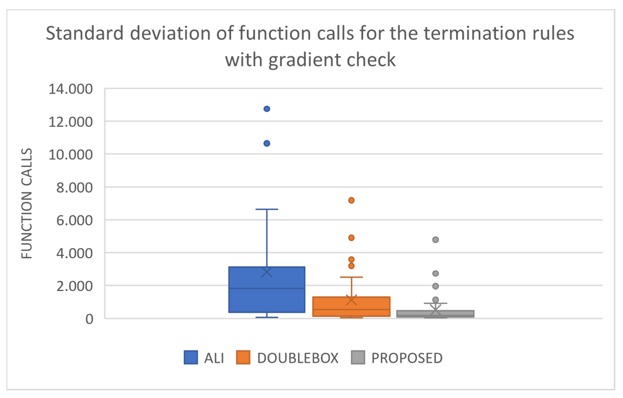
- The local optimization avoidance mechanism of the gradient check drastically reduces the required number of calls for each termination criterion while maintaining the success rate of the method at extremely high levels.
- 4.
- The proposed termination criterion is significantly superior to the other two with which the comparison was made. In addition, if the termination criterion is combined with the mechanism for avoiding local optimizations, then the gain in the number of calls grows even more.
4. Conclusions
Author Contributions
Funding
Institutional Review Board Statement
Informed Consent Statement
Data Availability Statement
Acknowledgments
Conflicts of Interest
References
- Yang, L.; Robin, D.; Sannibale, F.; Steier, C.; Wan, W. Global optimization of an accelerator lattice using multiobjective genetic algorithms. Nucl. Instrum. Methods Phys. Res. Accel. Spectrom. Detect. Assoc. Equip. 2009, 609, 50–57. [Google Scholar] [CrossRef]
- Iuliano, E. Global optimization of benchmark aerodynamic cases using physics-based surrogate models. Aerosp. Sci. Technol. 2017, 67, 273–286. [Google Scholar] [CrossRef]
- Schneider, P.I.; Santiago, X.G.; Soltwisch, V.; Hammerschmidt, M.; Burger, S.; Rockstuhl, C. Benchmarking Five Global Optimization Approaches for Nano-optical Shape Optimization and Parameter Reconstruction. ACS Photonics 2019, 6, 2726–2733. [Google Scholar] [CrossRef]
- Heiles, S.; Johnston, R.L. Global optimization of clusters using electronic structure methods. Int. J. Quantum Chem. 2013, 113, 2091–2109. [Google Scholar] [CrossRef]
- Shin, W.H.; Kim, J.K.; Kim, D.S.; Seok, C. GalaxyDock2: Protein-ligand docking using beta-complex and global optimization. J. Comput. Chem. 2013, 34, 2647–2656. [Google Scholar] [CrossRef] [PubMed]
- Marques, J.M.C.; Pereira, F.B.; Llanio-Trujillo, J.L.; Abreu, P.E.; Albertí, M.; Aguilar, A.; Bartolomei, F.P.F.M. A global optimization perspective on molecular clusters. Phil. Trans. R. Soc. A 2017, 375, 20160198. [Google Scholar] [CrossRef]
- Aguilar-Rivera, R.; Valenzuela-Rendón, M.; Rodríguez-Ortiz, J.J. Genetic algorithms and Darwinian approaches in financial applications: A survey. Expert Syst. Appl. 2015, 42, 7684–7697. [Google Scholar] [CrossRef]
- Hosseinnezhad, V.; Babaei, E. Economic load dispatch using θ-PSO. Int. J. Electr. Power Energy Syst. 2013, 49, 160–169. [Google Scholar] [CrossRef]
- Lee, E.K. Large-Scale Optimization-Based Classification Models in Medicine and Biology. Ann. Biomed. Eng. 2007, 35, 1095–1109. [Google Scholar] [CrossRef] [Green Version]
- Boutros, P.; Ewing, A.; Ellrott, K. Global optimization of somatic variant identification in cancer genomes with a global community challenge. Nat. Genet. 2014, 46, 318–319. [Google Scholar] [CrossRef] [Green Version]
- Wolfe, M.A. Interval methods for global optimization. Appl. Math. Comput. 1996, 75, 179–206. [Google Scholar]
- Reinking, J. GNSS-SNR water level estimation using global optimization based on interval analysis. J. Geod. 2016, 6, 80–92. [Google Scholar] [CrossRef]
- Price, W.L. Global optimization by controlled random search. J. Optim. Theory Appl. 1983, 40, 333–348. [Google Scholar] [CrossRef]
- Gupta, R.; Chandan, M. Use of “Controlled Random Search Technique for Global Optimization” in Animal Diet Problem. Int. Emerg. Technol. Adv. Eng. 2013, 3, 284–287. [Google Scholar]
- Charilogis, V.; Tsoulos, I.; Tzallas, A.; Anastasopoulos, N. An Improved Controlled Random Search Method. Symmetry 2021, 13, 1981. [Google Scholar] [CrossRef]
- Kirkpatrick, S.; Gelatt, C.D.; Vecchi, M.P. Optimization by simulated annealing. Science 1983, 220, 671–680. [Google Scholar] [CrossRef]
- Tavares, R.S.; Martins, T.C.; Tsuzuki, M.S.G. Simulated annealing with adaptive neighborhood: A case study in off-line robot path planning. Expert Syst. Appl. 2011, 38, 2951–2965. [Google Scholar] [CrossRef]
- Geng, X.; Chen, Z.; Yang, W.; Shi, D.; Zhao, K. Solving the traveling salesman problem based on an adaptive simulated annealing algorithm with greedy search. Appl. Soft Comput. 2011, 11, 3680–3689. [Google Scholar] [CrossRef]
- Storn, R.; Price, K. Differential Evolution—A Simple and Efficient Heuristic for Global Optimization over Continuous Spaces. J. Glob. Optim. 1997, 11, 341–359. [Google Scholar] [CrossRef]
- Liu, J.; Lampinen, J. A Fuzzy Adaptive Differential Evolution Algorithm. Soft Comput. 2005, 9, 448–462. [Google Scholar] [CrossRef]
- Kennedy, J.; Eberhart, R. Particle swarm optimization. In Proceedings of the ICNN’95—International Conference on Neural Networks, Perth, Australia, 1 December 1995; Volume 4, pp. 1942–1948. [Google Scholar]
- Poli, R.; Kennedy, J.K.; Blackwell, T. Particle swarm optimization An Overview. Swarm Intell. 2007, 1, 33–57. [Google Scholar] [CrossRef]
- Trelea, I.C. The particle swarm optimization algorithm: Convergence analysis and parameter selection. Inf. Process. Lett. 2003, 85, 317–325. [Google Scholar] [CrossRef]
- Dorigo, M.; Birattari, M.; Stutzle, T. Ant colony optimization. IEEE Comput. Intell. Mag. 2006, 1, 28–39. [Google Scholar] [CrossRef]
- Socha, K.; Dorigo, M. Ant colony optimization for continuous domains. Eur. J. Oper. Res. 2008, 185, 1155–1173. [Google Scholar] [CrossRef] [Green Version]
- Goldberg, D. Genetic Algorithms in Search, Optimization and Machine Learning; Addison-Wesley Publishing Company: Reading, MA, USA, 1989. [Google Scholar]
- Hamblin, S. On the practical usage of genetic algorithms in ecology and evolution. Methods Ecol. Evol. 2013, 4, 184–194. [Google Scholar] [CrossRef]
- Grady, S.A.; Hussaini, M.Y.; Abdullah, M.M. Placement of wind turbines using genetic algorithms. Renew. Energy 2005, 30, 259–270. [Google Scholar] [CrossRef]
- Zhou, Y.; Tan, Y. GPU-based parallel particle swarm optimization. In Proceedings of the 2009 IEEE Congress on Evolutionary Computation, Trondheim, Norway, 18–21 May 2009; pp. 1493–1500. [Google Scholar]
- Dawson, L.; Stewart, I. Improving Ant Colony Optimization performance on the GPU using CUDA. In Proceedings of the 2013 IEEE Congress on Evolutionary Computation, Cancun, Mexico, 20–23 June 2013; pp. 1901–1908. [Google Scholar]
- Barkalov, K.; Gergel, V. Parallel global optimization on GPU. J. Glob. Optim. 2016, 66, 3–20. [Google Scholar] [CrossRef]
- Lepagnot, I.B.J.; Siarry, P. A survey on optimization metaheuristics. Inf. Sci. 2013, 237, 82–117. [Google Scholar]
- Dokeroglu, T.; Sevinc, E.; Kucukyilmaz, T.; Cosar, A. A survey on new generation metaheuristic algorithms. Comput. Ind. Eng. 2019, 137, 106040. [Google Scholar] [CrossRef]
- Hussain, K.; Salleh, M.N.M.; Cheng, S.; Shi, Y. Metaheuristic research: A comprehensive survey. Artif. Intell. Rev. 2019, 52, 2191–2233. [Google Scholar] [CrossRef] [Green Version]
- Jain, N.K.; Nangia, U.; Jain, J. A Review of Particle Swarm Optimization. J. Inst. Eng. India Ser. B 2018, 99, 407–411. [Google Scholar] [CrossRef]
- Khare, l.; Rangnekar, S. A review of particle swarm optimization and its applications in Solar Photovoltaic system. Appl. Soft Comput. 2013, 13, 2997–3306. [Google Scholar] [CrossRef]
- Meneses, A.A.D.; Dornellas, M.; Schirru, M.R. Particle Swarm Optimization applied to the nuclear reload problem of a Pressurized Water Reactor. Progress Nucl. Energy 2009, 51, 319–326. [Google Scholar] [CrossRef]
- Shaw, R.; Srivastava, S. Particle swarm optimization: A new tool to invert geophysical data. Geophysics 2007, 72, F75–F83. [Google Scholar] [CrossRef]
- Ourique, C.O.; Biscaia, E.C.; Pinto, J.C. The use of particle swarm optimization for dynamical analysis in chemical processes. Comput. Chem. Eng. 2002, 26, 1783–1793. [Google Scholar] [CrossRef]
- Fang, H.; Zhou, J.; Wang, Z. Hybrid method integrating machine learning and particle swarm optimization for smart chemical process operations. Front. Chem. Sci. Eng. 2022, 16, 274–287. [Google Scholar] [CrossRef]
- Wachowiak, M.P.; Smolikova, R.; Zheng, Y.J.M.; Zurada, A.S.E. An approach to multimodal biomedical image registration utilizing particle swarm optimization. IEEE Trans. Evol. Comput. 2004, 8, 289–301. [Google Scholar] [CrossRef]
- Marinakis, Y.; Marinaki, M.; Dounias, G. Particle swarm optimization for pap-smear diagnosis. Expert Syst. Appl. 2008, 35, 1645–1656. [Google Scholar] [CrossRef]
- Park, J.; Jeong, Y.; Shin, J.; Lee, K. An Improved Particle Swarm Optimization for Nonconvex Economic Dispatch Problems. IEEE Trans. Power Syst. 2010, 25, 156–166. [Google Scholar] [CrossRef]
- Clerc, M. The swarm and the queen: Towsrds a deterministic and adaptive particle swarm optimization. In Proceedings of the 1999 Congress on Evolutionary Computation-CEC99 (Cat. No. 99TH8406), Washington, DC, USA, 6–9 July 1999; Volume 3, pp. 1951–1957. [Google Scholar]
- Juan, H.; Laihang, Y.; Kaiqi, Z. Enhanced Self-Adaptive Search Capability Particle Swarm Optimization. In Proceedings of the 2008 Eighth International Conference on Intelligent Systems Design and Applications, Kaohsiung, Taiwan, 28 November 2008; pp. 49–55. [Google Scholar]
- Hou, Z.X. Wiener model identification based on adaptive particle swarm optimization. In Proceedings of the 2008 International Conference on Machine Learning and Cybernetics, Kunming, China, 10 January 2008; pp. 1041–1045. [Google Scholar]
- Ratnaweera, A.; Halgamuge, S.K.; Watson, H.C. Self-organizing hierarchical particle swarm optimizer with time-varying acceleration coefficients. IEEE Trans. Evol. Comput. 2004, 8, 240–255. [Google Scholar] [CrossRef]
- Stacey, A.; Jancic, M.; Grundy, I. Particle swarm optimization with mutation. In Proceedings of the 2003 Congress on Evolutionary Computation, CEC ’03, Canberra, Australia, 12 December 2004; pp. 1425–1430. [Google Scholar]
- Pant, M.; Thangaraj, R.; Abraham, A. Particle Swarm Optimization Using Adaptive Mutation. In Proceedings of the 2008 19th International Workshop on Database and Expert Systems Applications, Turin, Italy, 1–5 September 2008; pp. 519–523. [Google Scholar]
- Higashi, N.; Iba, H. Particle swarm optimization with Gaussian mutation. In Proceedings of the 2003 IEEE Swarm Intelligence Symposium. SIS’03 (Cat. No.03EX706), Indianapolis, IN, USA, 26–26 April 2003; pp. 72–79. [Google Scholar]
- Engelbrecht, A. Particle swarm optimization: Velocity initialization. In Proceedings of the 2012 IEEE Congress on Evolutionary Computation, Brisbane, Australia, 10–15 June 2012; pp. 1–8. [Google Scholar]
- Liu, B.; Wang, L.; Jin, Y.H.; Tang, F.; Huang, D.X. Improved particle swarm optimization combined with chaos. Chaos Solitions Fract. 2005, 25, 1261–1271. [Google Scholar] [CrossRef]
- Shi, X.H.; Liang, Y.C.; Lee, H.P.; Lu, C.; Wang, L.M. An improved GA and a novel PSO-GA based hybrid algorithm. Inf. Proc. Lett. 2005, 93, 255–261. [Google Scholar] [CrossRef]
- Garg, H. A hybrid PSO-GA algorithm for constrained optimization problems. Appl. Math. Comput. 2016, 274, 292–305. [Google Scholar] [CrossRef]
- Schutte, J.F.; Reinbolt, J.A.; Fregly, B.J.; Haftka, R.T.; George, A.D. Parallel global optimization with the particle swarm algorithm. Int. J. Numer. Meth. Eng. 2004, 61, 2296–2315. [Google Scholar] [CrossRef] [Green Version]
- Koh, B.; George, A.D.; Haftka, R.T.; Fregly, B.J. Parallel asynchronous particle swarm optimization. Int. J. Numer. Meth. Eng. 2006, 67, 578–595. [Google Scholar] [CrossRef]
- Venter, G.; Sobieszczanski-Sobieski, J. Parallel Particle Swarm Optimization Algorithm Accelerated by Asynchronous Evaluations. J. Aerosp. Comput. Inf. Commun. 2006, 3, 123–137. [Google Scholar] [CrossRef] [Green Version]
- Gaing, Z.L. Particle swarm optimization to solving the economic dispatch considering the generator constraints. IEEE Trans. Power Syst. 2003, 18, 1187–1195. [Google Scholar] [CrossRef]
- Yang, X.; Yuan, J.; Yuan, J.; Mao, H. A modified particle swarm optimizer with dynamic adaptation. Appl. Math. Comput. 2007, 189, 1205–1213. [Google Scholar] [CrossRef]
- Jiang, Y.; Hu, T.; Huang, C.; Wu, X. An improved particle swarm optimization algorithm. Appl. Math. Comput. 2007, 193, 231–239. [Google Scholar] [CrossRef]
- Bogdanova, A.; Junior, J.P.; Aranha, C. Franken-Swarm: Grammatical Evolution for the Automatic Generation of Swarm-like Meta-Heuristics. In Proceedings of the Genetic and Evolutionary Computation Conference Companion, New York, NY, USA, 15 July 2018; pp. 411–412. [Google Scholar]
- O’Neill, M.; Ryan, C. Grammatical evolution. IEEE Trans. Evol. Comput. 2001, 5, 349–358. [Google Scholar] [CrossRef] [Green Version]
- Pan, X.; Xue, L.; Lu, Y. Hybrid particle swarm optimization with simulated annealing. Multimed Tools Appl. 2019, 78, 29921–29936. [Google Scholar] [CrossRef]
- Mughal, M.A.; Ma, Q.; Xiao, C. Photovoltaic Cell Parameter Estimation Using Hybrid Particle Swarm Optimization and Simulated Annealing. Energies 2017, 10, 1213. [Google Scholar] [CrossRef] [Green Version]
- Lin, G.H.; Zhang, J.; Liu, Z.H. Hybrid particle swarm optimization with differential evolution for numerical and engineering optimization. Int. J. Autom. Comput. 2018, 15, 103–114. [Google Scholar] [CrossRef]
- Epitropakis, M.G.; Plagianakos, V.P.; Vrahatis, M.N. Evolving cognitive and social experience in Particle Swarm Optimization through Differential Evolution: A hybrid approach. Inf. Sci. 2012, 216, 50–92. [Google Scholar] [CrossRef] [Green Version]
- Wang, W.; Wu, J.M.; Liu, J.H. A Particle Swarm Optimization Based on Chaotic Neighborhood Search to Avoid Premature Convergence. In Proceedings of the 2009 Third International Conference on Genetic and Evolutionary Computing, Washington, DC, USA, 14 October 2009; pp. 633–636. [Google Scholar]
- Eberhart, R.C.; Shi, Y.H. Tracking and optimizing dynamic systems with particle swarms. In Proceedings of the Congress on Evolutionary Computation, Seoul, Korea, 27–30 May 2001. [Google Scholar]
- Shi, Y.H.; Eberhart, R.C. Empirical study of particle swarm optimization. In Proceedings of the Congress on Evolutionary Computation, Washington, DC, USA, 6–9 July 1999. [Google Scholar]
- Shi, Y.H.; Eberhart, R.C. Experimental study of particle swarm optimization. In Proceedings of the SCI2000 Conference, Orlando, FL, USA, 23–26 July 2000. [Google Scholar]
- Zheng, Y.; Ma, L.; Zhang, L.; Qian, J. Empirical study of particle swarm optimizer with an increasing inertia weight. IEEE Congr. Evol. Comput. 2003, 1, 221–226. [Google Scholar]
- Zheng, Y.; Ma, L.; Zhang, L.; Qian, J. On the convergence analysis and param- eter selection in particle swarm optimization. In Proceedings of the Second International Conference on Machine Learning and Cybernetics, Xi’an, China, 5 November 2003. [Google Scholar]
- Tsoulos, I.G.; Lagaris, I.E. MinFinder: Locating all the local minima of a function. Comput. Phys. Commun. 2006, 174, 166–179. [Google Scholar] [CrossRef] [Green Version]
- Ali, M.M.; Kaelo, P. Improved particle swarm algorithms for global optimization. Appl. Math. Comput. 2008, 196, 578–593. [Google Scholar] [CrossRef]
- Tsoulos, I.G. Modifications of real code genetic algorithm for global optimization. Appl. Math. Comput. 2008, 203, 598–607. [Google Scholar] [CrossRef]
- Ali, M.M.; Khompatraporn, C.; Zabinsky, Z.B. A Numerical Evaluation of Several Stochastic Algorithms on Selected Continuous Global Optimization Test Problems. J. Glob. Optim. 2005, 31, 635–672. [Google Scholar] [CrossRef]
- Floudas, C.A.; Pardalos, P.M.; Adjiman, C.; Esposoto, W.; Gümüs, Z.; Harding, S.; Klepeis, J.; Meyer, C.; Schweiger, C. Handbook of Test Problems in Local and Global Optimization; Kluwer Academic Publishers: Dordrecht, The Netherlands, 1999. [Google Scholar]
- Koyuncu, H.; Ceylan, R. A PSO based approach: Scout particle swarm algorithm for continuous global optimization problems. J. Comput. Des. Eng. 2019, 6, 129–142. [Google Scholar] [CrossRef]
- Siarry, P.; Berthiau, G.; François, D.; Haussy, J. Enhanced simulated annealing for globally minimizing functions of many-continuous variables. ACM Trans. Math. Softw. 1997, 23, 209–228. [Google Scholar] [CrossRef]
- Tsoulos, I.G.; Lagaris, I.E. GenMin: An enhanced genetic algorithm for global optimization. Comput. Phys. Commun. 2008, 178, 843–851. [Google Scholar] [CrossRef]
- Gaviano, M.; Ksasov, D.E.; Lera, D.; Sergeyev, Y.D. Software for generation of classes of test functions with known local and global minima for global optimization. ACM Trans. Math. Softw. 2003, 29, 469–480. [Google Scholar] [CrossRef]
- Lennard-Jones, J.E. On the Determination of Molecular Fields. Proc. R. Soc. Lond. A 1924, 106, 463–477. [Google Scholar]
- Powell, M.J.D. A Tolerant Algorithm for Linearly Constrained Optimization Calculations. Math. Program. 1989, 45, 547–566. [Google Scholar] [CrossRef]


| Parameter | Value |
|---|---|
| m | 100 |
| 100 | |
| 0.05 | |
| 1.0 | |
| 1.0 | |
| 0.4 | |
| 0.9 | |
| 0.001 | |
| 15 |
| FUNCTION | I1 | I2 | I3 | IP |
|---|---|---|---|---|
| BF1 | 24,929 | 22,874 | 18,739 | 22,088 |
| BF2 | 24,043 | 22,254 | 17,172 | 20,743 |
| BRANIN | 17,691 | 16,205 | 13,397 | 12,471 |
| CM4 | 20,117 | 22,568 | 26,867 | 14,941 |
| CAMEL | 19,474 | 17,813 | 14,461 | 13,492 |
| EASOM | 13,327 | 13,106 | 9969 | 9212 |
| EXP2 | 6339 | 8243 | 7853 | 3501 |
| EXP4 | 7816 | 10,066 | 10,900 | 4458 |
| EXP8 | 8667 | 10,937 | 13,126 | 4761 |
| EXP16 | 8748 | 11,402 | 15,754 | 5098 |
| EXP32 | 9567 | 12,323 | 18,189 | 5471 |
| GKLS250 | 10,907 | 12,562 | 9673 | 8552 |
| GKLS2100 | 12,960 | 13,403 | 9930 | 9541 |
| GKLS350 | 15,410(0.97) | 14,722 | 10,542 | 9298 |
| GKLS3100 | 16,639 | 14,495 | 10,412 | 13,075(0.97) |
| GOLDSTEIN | 20,437 | 22,877 | 16,410 | 8935 |
| GRIEWANK2 | 27,620 | 24,230 | 18,473 | 20,133 |
| HANSEN | 21,513 | 20,279 | 16,326 | 15,046 |
| HARTMAN3 | 16,233 | 17,152 | 12,305 | 6511 |
| HARTMAN6 | 47,038 | 48,947 | 46,852 | 23,431 |
| POTENTIAL3 | 31,684 | 32,175 | 36,930 | 24,463 |
| POTENTIAL4 | 184,602 | 181,231 | 168,962 | 129,267 |
| POTENTIAL5 | 74,508 | 70,519 | 76,890 | 54,042 |
| RASTRIGIN | 23,574 | 20,865 | 15,596 | 16,198 |
| ROSENBROCK4 | 145,178 | 161,136 | 160,341 | 129,891 |
| ROSENBROCK8 | 95,290 | 97,035 | 96,687 | 80,408 |
| ROSENBCROK16 | 118,614 | 116,454 | 115,122 | 97,004 |
| SHEKEL5 | 27,458 | 27,088 | 25,927 | 18,036 |
| SHEKEL7 | 27,521 | 27,271 | 25,967 | 18,805 |
| SHEKEL10 | 29,699(0.97) | 28,082 | 25,511 | 20,823 |
| TEST2N4 | 26,740 | 27,050 | 22,905 | 19,495 |
| TEST2N5 | 20,243(0.97) | 20,290 | 17,729 | 16,024(0.97) |
| TEST2N6 | 33,118 | 33,366 | 30,118 | 25,235(0.93) |
| TEST2N7 | 23,266(0.90) | 22,804 | 21,294 | 18,218(0.90) |
| SINU4 | 17,035 | 20,487 | 18,971 | 11,079 |
| SINU8 | 22,827 | 27,176 | 27,732 | 12,379 |
| SINU16 | 31,055 | 35,998 | 42,984 | 15,692 |
| SINU32 | 44,736(0.97) | 51,624 | 82,114 | 25,991 |
| TEST30N3 | 18,733 | 20,119 | 17,803 | 17,543 |
| TEST30N4 | 20,348 | 22,191 | 20,679 | 20,085 |
| TOTAL | 1,365,704(0.99) | 1,399,419 | 1,367,612 | 1,001,436(0.99) |
| FUNCTION | I1 | I2 | I3 | IP |
|---|---|---|---|---|
| BF1 | 9709 | 8918 | 9531 | 10,932 |
| BF2 | 10,196 | 9588 | 9089 | 10,730 |
| BRANIN | 10,718 | 9597 | 9813 | 9501 |
| CM4 | 6242 | 7503 | 12,531 | 6985 |
| CAMEL | 10,422 | 9306 | 8491 | 9624 |
| EASOM | 11,565 | 11,366 | 8497 | 8196 |
| EXP2 | 3364 | 4443 | 4558 | 1926 |
| EXP4 | 3558 | 4767 | 6023 | 2122 |
| EXP8 | 3716 | 4787 | 7753 | 2186 |
| EXP16 | 3784 | 5076 | 9696 | 2211 |
| EXP32 | 4137 | 5698 | 11,379 | 2323 |
| GKLS250 | 5917 | 7080 | 7517 | 5273 |
| GKLS2100 | 6843 | 8261 | 7449 | 7296 |
| GKLS350 | 6845 | 8076 | 7833 | 5881(0.97) |
| GKLS3100 | 10,290(0.93) | 10,187 | 7828 | 8066(0.97) |
| GOLDSTEIN | 7977 | 9035 | 8505 | 4381 |
| GRIEWANK2 | 12,567 | 12,222 | 12,000 | 12,037 |
| HANSEN | 13,441 | 13,360 | 11,876 | 10,818 |
| HARTMAN3 | 9758 | 9548 | 8123 | 4114 |
| HARTMAN6 | 12,893(0.90) | 12,889(0.93) | 22,309 | 10,126(0.93) |
| POTENTIAL3 | 17,912 | 16,420 | 21,904 | 15,969 |
| POTENTIAL4 | 73,629 | 64,886 | 95,707 | 67,084 |
| POTENTIAL5 | 40,585 | 35,239 | 47,807 | 33,661 |
| RASTRIGIN | 11,305 | 10,101 | 11,141 | 10,046 |
| ROSENBROCK4 | 18,115 | 21,919 | 38,407 | 43,093 |
| ROSENBROCK8 | 12,869 | 14,192 | 31,923 | 25,405 |
| ROSENBCROK16 | 12,096 | 13,023 | 38,486 | 23,165 |
| SHEKEL5 | 10,347 | 11,466 | 14,446 | 11,802 |
| SHEKEL7 | 11,511 | 10,521 | 13,944 | 10,399 |
| SHEKEL10 | 10,834 | 10,842 | 13,785 | 12,253 |
| TEST2N4 | 11,133 | 10,869 | 12,161 | 11,546 |
| TEST2N5 | 10,923(0.97) | 10,315 | 10,868 | 11,072(0.97) |
| TEST2N6 | 12,331(0.97) | 12,345 | 14,123 | 15,652 |
| TEST2N7 | 11,342(0.93) | 11,354 | 12,118 | 12,370(0.93) |
| SINU4 | 7724 | 9845 | 12,294 | 6575 |
| SINU8 | 8468 | 10,969 | 18,122 | 5382 |
| SINU16 | 9334 | 13,213 | 31,589 | 9294 |
| SINU32 | 13,290 | 17,502(0.97) | 63,111(0.97) | 14,959 |
| TEST30N3 | 12,675 | 12,954 | 12,472 | 12,482 |
| TEST30N4 | 13,964 | 14,903 | 14,999 | 15,389 |
| TOTAL | 494,119(0.99) | 504,585(0.99) | 720,208(0.99) | 502,326(0.99) |
| FUNCTION | I1 | I2 | I3 | IP |
|---|---|---|---|---|
| BF1 | 6807 | 6866 | 6712 | 6757 |
| BF2 | 6102 | 6150 | 6057 | 6207 |
| BRANIN | 4551 | 4596 | 4470 | 4435 |
| CM4 | 9814 | 10,101 | 9580 | 9342 |
| CAMEL | 5055 | 5202 | 4897 | 5004 |
| EASOM | 2975 | 2788 | 3014 | 3000 |
| EXP2 | 4436 | 4541 | 4377 | 4543 |
| EXP4 | 5443 | 5562 | 5331 | 5290 |
| EXP8 | 5682 | 5754 | 5614 | 5504 |
| EXP16 | 5707 | 5799 | 5638 | 5526 |
| EXP32 | 5871 | 5797 | 5769 | 5659 |
| GKLS250 | 3973 | 3906 | 3971 | 3921 |
| GKLS2100 | 4009 | 3862 | 4073 | 3958 |
| GKLS350 | 4558 | 3965 | 4525(0.97) | 4266 |
| GKLS3100 | 4701(0.87) | 4266 | 4361(0.90) | 4465 |
| GOLDSTEIN | 10,259 | 9145 | 7945 | 7625 |
| GRIEWANK2 | 5932 | 6194 | 5700 | 5915 |
| HANSEN | 6386 | 6260 | 5688(0.97) | 5874 |
| HARTMAN3 | 4681 | 4694 | 4625 | 4675 |
| HARTMAN6 | 14,245 | 14,091 | 13,793 | 13,825 |
| POTENTIAL3 | 7219 | 7206 | 7532 | 7234 |
| POTENTIAL4 | 38,053 | 37,924 | 38,421 | 38,897 |
| POTENTIAL5 | 15,196 | 14,459 | 15,708 | 15,358 |
| RASTRIGIN | 5915 | 5797 | 5944(0.83) | 5844 |
| ROSENBROCK4 | 91,574 | 101,485 | 117,512 | 76,367 |
| ROSENBROCK8 | 66,648 | 61,974 | 58,831 | 41,591 |
| ROSENBCROK16 | 62,029 | 54,550 | 63,406 | 55,800 |
| SHEKEL5 | 9119 | 10,271(0.97) | 8975 | 8538 |
| SHEKEL7 | 9197 | 9831 | 9638 | 8732 |
| SHEKEL10 | 10,417 | 10,449 | 9373 | 9721(0.90) |
| TEST2N4 | 8512 | 8272 | 8884 | 7992 |
| TEST2N5 | 5793 | 5704 | 5511(0.90) | 5515 |
| TEST2N6 | 9797(0.93) | 9731 | 9657(0.83) | 9666(0.97) |
| TEST2N7 | 6435(0.80) | 6659 | 6713(0.77) | 5990(0.87) |
| SINU4 | 7567 | 7774 | 7334 | 7063 |
| SINU8 | 9882 | 10,083 | 9643 | 9331 |
| SINU16 | 12,750 | 12,947 | 12,569 | 12,207 |
| SINU32 | 20,164 | 21,112 | 19,684(0.90) | 19,239 |
| TEST30N3 | 6388 | 7942 | 5934 | 5855 |
| TEST30N4 | 7611 | 9251 | 6385 | 8284 |
| TOTAL | 531,453(0.99) | 532,690(0.99) | 543,794(0.98) | 475,015(0.99) |
| FUNCTION | I1 | I2 | I3 | IP |
|---|---|---|---|---|
| BF1 | 3296 | 3038 | 3063 | 3003 |
| BF2 | 2922 | 2762 | 2863 | 2845 |
| BRANIN | 2562 | 2641 | 2538 | 2564 |
| CM4 | 3569 | 4277 | 2944 | 3230 |
| CAMEL | 2646 | 2854 | 2467 | 2577 |
| EASOM | 2490 | 2390 | 2479 | 2464 |
| EXP2 | 2377 | 2489 | 2261 | 2315 |
| EXP4 | 2456 | 2669 | 2282 | 2389 |
| EXP8 | 2429 | 2671 | 2268 | 2385 |
| EXP16 | 2358 | 2569 | 2227 | 2326 |
| EXP32 | 2337 | 2533 | 2248 | 2312 |
| GKLS250 | 2394 | 2535 | 2274 | 2321 |
| GKLS2100 | 2384 | 2511 | 2267 | 2333 |
| GKLS350 | 2492 | 2410 | 2212 | 2339 |
| GKLS3100 | 2800(0.90) | 2708 | 2648(0.83) | 2571 |
| GOLDSTEIN | 3161 | 3701 | 3166 | 2799 |
| GRIEWANK2 | 3910 | 4520 | 3543 | 3641 |
| HANSEN | 4409 | 4268 | 3755 | 4325 |
| HARTMAN3 | 2423 | 2518 | 2374 | 2425 |
| HARTMAN6 | 3913 | 4390 | 4199(0.93) | 3700 |
| POTENTIAL3 | 3951 | 4093 | 4482 | 4021 |
| POTENTIAL4 | 18,555 | 19,559 | 19,506 | 18,691 |
| POTENTIAL5 | 8771 | 8397 | 9677 | 9154 |
| RASTRIGIN | 3111 | 3244(0.97) | 3031 | 3146 |
| ROSENBROCK4 | 9729 | 12,980 | 11,453 | 8587 |
| ROSENBROCK8 | 4987 | 6738 | 4688 | 5512 |
| ROSENBCROK16 | 4410 | 5939 | 4553 | 4002 |
| SHEKEL5 | 3906 | 4095 | 3203 | 3495 |
| SHEKEL7 | 3119 | 3965 | 2950 | 3528 |
| SHEKEL10 | 3497(0.97) | 4464 | 3142(0.97) | 3353 |
| TEST2N4 | 3468(0.97) | 4059 | 4167 | 3881(0.93) |
| TEST2N5 | 3318(0.97) | 3786 | 2926(0.90) | 3157(0.97) |
| TEST2N6 | 4523(0.93) | 5046(0.93) | 5537(0.83) | 4066(0.97) |
| TEST2N7 | 3364(0.80) | 4191(0.90) | 4183(0.80) | 3315(0.87) |
| SINU4 | 3173 | 3807 | 2610 | 3004 |
| SINU8 | 3055 | 3742 | 2592 | 2857 |
| SINU16 | 3160 | 3746 | 3854 | 3290 |
| SINU32 | 6613 | 7377 | 6327 | 6450 |
| TEST30N3 | 5129 | 6367 | 5605 | 4451 |
| TEST30N4 | 5649 | 6441 | 6074 | 5543 |
| TOTAL | 162,816(0.99) | 182,490(0.99) | 164,638(0.98) | 158,367(0.99) |
| FUNCTION | I1 | I2 | I3 | IP |
|---|---|---|---|---|
| BF1 | 5305 | 5326 | 5240 | 5209 |
| BF2 | 4760 | 4841 | 4750 | 4856 |
| BRANIN | 3599 | 3703 | 3520 | 3443 |
| CM4 | 7674 | 7835 | 7430 | 7057 |
| CAMEL | 3996 | 4131 | 3864 | 3825 |
| EASOM | 2370 | 2292 | 2425 | 2478 |
| EXP2 | 3528 | 3613 | 3455 | 3675 |
| EXP4 | 4292 | 4350 | 4178 | 4020 |
| EXP8 | 4579 | 4632 | 4515 | 4278 |
| EXP16 | 4576 | 4637 | 4505 | 4236 |
| EXP32 | 4692 | 4771 | 4588 | 4296 |
| GKLS250 | 3105 | 3065 | 3115 | 3024 |
| GKLS2100 | 3193 | 3049 | 3193 | 3099 |
| GKLS350 | 3308 | 3000 | 3560 | 3401 |
| GKLS3100 | 2935(0.97) | 2777 | 3158(0.83) | 3088 |
| GOLDSTEIN | 5534 | 5595 | 5332 | 5265 |
| GRIEWANK2 | 4225 | 4332 | 4413 | 4489 |
| HANSEN | 3865 | 3762 | 3824 | 3769 |
| HARTMAN3 | 3724 | 3770 | 3714 | 3705 |
| HARTMAN6 | 11,901(0.97) | 11,829(0.97) | 11,386 | 10,573 |
| POTENTIAL3 | 5910 | 5850 | 6134 | 6501 |
| POTENTIAL4 | 30,880 | 30,570 | 31,180 | 30,682 |
| POTENTIAL5 | 12,021 | 11,643 | 12,521 | 13,475 |
| RASTRIGIN | 4583 | 4595 | 4625 | 4360 |
| ROSENBROCK4 | 58,299 | 61,266 | 55,759 | 35,517 |
| ROSENBROCK8 | 31,778 | 30,888 | 30,989 | 22,055 |
| ROSENBCROK16 | 32,719 | 30,503 | 30,957 | 24,478 |
| SHEKEL5 | 6806 | 7047(0.97) | 6636 | 6233 |
| SHEKEL7 | 6807 | 7001 | 6626 | 6270 |
| SHEKEL10 | 6774 | 6987 | 6583 | 6534 |
| TEST2N4 | 6111 | 6127 | 5909 | 5893 |
| TEST2N5 | 4455(0.97) | 4558 | 4372(0.97) | 4271(0.93) |
| TEST2N6 | 7446(0.97) | 7419 | 7218(0.87) | 7122(0.93) |
| TEST2N7 | 4992(0.90) | 5057 | 4888(0.83) | 4680(0.90) |
| SINU4 | 5948 | 6043 | 5750 | 5229 |
| SINU8 | 7965 | 8095 | 7778 | 6963 |
| SINU16 | 10,121 | 10,252 | 9968 | 9219 |
| SINU32 | 16,093 | 16,509 | 15,663 | 14,478 |
| TEST30N3 | 4331 | 4953 | 4230 | 3957 |
| TEST30N4 | 6290 | 6341 | 4288 | 4717 |
| TOTAL | 361,490(0.99) | 363,013(0.99) | 352,239(0.99) | 310,420(0.99) |
| FUNCTION | I1 | I2 | I3 | IP |
|---|---|---|---|---|
| BF1 | 2276 | 2379 | 2266 | 2250 |
| BF2 | 2157 | 2274 | 2098 | 2191 |
| BRANIN | 2132 | 2178 | 2051 | 2170 |
| CM4 | 3098 | 3717 | 2538 | 2791 |
| CAMEL | 2198 | 2335 | 1974 | 2058 |
| EASOM | 2007 | 2011 | 2031 | 2084 |
| EXP2 | 1952 | 2030 | 1842 | 1861 |
| EXP4 | 2046 | 2266 | 1877 | 1909 |
| EXP8 | 1990 | 2240 | 1849 | 1879 |
| EXP16 | 1944 | 2110 | 1828 | 1838 |
| EXP32 | 1953 | 2126 | 1859 | 1867 |
| GKLS250 | 1982 | 2079 | 1850 | 1900 |
| GKLS2100 | 1983 | 2064 | 1859 | 1891 |
| GKLS350 | 1882 | 1944 | 1793 | 1831 |
| GKLS3100 | 1898 | 1909(0.97) | 1850(0.83) | 1833(0.83) |
| GOLDSTEIN | 2523 | 2670 | 2110 | 2164 |
| GRIEWANK2 | 2893 | 2885 | 2791 | 2681 |
| HANSEN | 2766 | 2879 | 2731 | 2804 |
| HARTMAN3 | 1988 | 2093 | 1949 | 2015 |
| HARTMAN6 | 3366 | 3871(0.97) | 2767 | 3133 |
| POTENTIAL3 | 3312 | 3487 | 3613 | 3892 |
| POTENTIAL4 | 15,392 | 16,390 | 16,223 | 17,497 |
| POTENTIAL5 | 7109 | 7104 | 7732 | 8477 |
| RASTRIGIN | 2591 | 2648 | 2474 | 2732 |
| ROSENBROCK4 | 8023 | 12,179 | 4433 | 6025 |
| ROSENBROCK8 | 4376 | 6081 | 2721 | 3314 |
| ROSENBCROK16 | 3643 | 4954 | 2746 | 2485 |
| SHEKEL5 | 2849 | 3296 | 2274 | 2390 |
| SHEKEL7 | 2696 | 3294 | 2262 | 2283 |
| SHEKEL10 | 2624 | 3251 | 2338(0.93) | 2359 |
| TEST2N4 | 2536 | 2637 | 2427 | 2782 |
| TEST2N5 | 2266(0.97) | 2336(0.97) | 2163(0.90) | 2342(0.90) |
| TEST2N6 | 2724(0.93) | 2832 | 2694(0.80) | 3133(0.90) |
| TEST2N7 | 2283(0.80) | 2370 | 2279(0.80) | 2585(0.90) |
| SINU4 | 2789 | 3245 | 2228 | 2436 |
| SINU8 | 2601 | 3151 | 2233 | 2348 |
| SINU16 | 2721 | 3086 | 2443 | 2624 |
| SINU32 | 4652 | 5135 | 4086 | 4089 |
| TEST30N3 | 3031 | 3349 | 3007 | 2562 |
| TEST30N4 | 3747 | 3797 | 3250 | 3237 |
| TOTAL | 126,999(0.99) | 142,682(0.99) | 115,539(0.98) | 122,742(0.99) |
Publisher’s Note: MDPI stays neutral with regard to jurisdictional claims in published maps and institutional affiliations. |
© 2022 by the authors. Licensee MDPI, Basel, Switzerland. This article is an open access article distributed under the terms and conditions of the Creative Commons Attribution (CC BY) license (https://creativecommons.org/licenses/by/4.0/).
Share and Cite
Charilogis, V.; Tsoulos, I.G. Toward an Ideal Particle Swarm Optimizer for Multidimensional Functions. Information 2022, 13, 217. https://doi.org/10.3390/info13050217
Charilogis V, Tsoulos IG. Toward an Ideal Particle Swarm Optimizer for Multidimensional Functions. Information. 2022; 13(5):217. https://doi.org/10.3390/info13050217
Chicago/Turabian StyleCharilogis, Vasileios, and Ioannis G. Tsoulos. 2022. "Toward an Ideal Particle Swarm Optimizer for Multidimensional Functions" Information 13, no. 5: 217. https://doi.org/10.3390/info13050217