Explainable Deep Learning Approach for Multi-Class Brain Magnetic Resonance Imaging Tumor Classification and Localization Using Gradient-Weighted Class Activation Mapping

Abstract

Brain tumors (BT) present a considerable global health concern because of their high mortality rates across diverse age groups. A delay in diagnosing BT can lead to death. Therefore, a timely and accurate diagnosis through magnetic resonance imaging (MRI) is crucial. A radiologist makes the final decision to identify the tumor through MRI. However, manual assessments are flawed, time-consuming, and rely on experienced radiologists or neurologists to identify and diagnose a BT. Computer-aided classification models often lack performance and explainability for clinical translation, particularly in neuroscience research, resulting in physicians perceiving the model results as inadequate due to the black box model. Explainable deep learning (XDL) can advance neuroscientific research and healthcare tasks. To enhance the explainability of deep learning (DL) and provide diagnostic support, we propose a new classification and localization model, combining existing methods to enhance the explainability of DL and provide diagnostic support. We adopt a pre-trained visual geometry group (pre-trained-VGG-19), scratch-VGG-19, and EfficientNet model that runs a modified form of the class activation mapping (CAM), gradient-weighted class activation mapping (Grad-CAM) and Grad-CAM++ algorithms. These algorithms, introduced into a convolutional neural network (CNN), uncover a crucial part of the classification and can provide an explanatory interface for diagnosing BT. The experimental results demonstrate that the pre-trained-VGG-19 with Grad-CAM provides better classification and visualization results than the scratch-VGG-19, EfficientNet, and cutting-edge DL techniques regarding visual and quantitative evaluations with increased accuracy. The proposed approach may contribute to reducing the diagnostic uncertainty and validating BT classification.

1. Introduction

A brain tumor (BT) develops due to the abnormal growth of brain tissue which can harm brain cells [1,2]. It is a severe neurological disorder affecting people of all ages and genders [3,4,5]. The brain controls the functionality of the entire body, and tumors can alter both the behavior and structure of the brain. Therefore, brain damage can be harmful to the body [6]. According to projections by the American Cancer Society, there will be 1,958,310 cancer cases and 609,820 cancer-related deaths in the United States by 2023 [7]. Thus, early and accurate diagnosis through magnetic resonance imaging (MRI) can enhance the evaluation and prognosis of BT. Brain cancer can be treated in various ways: mainly including surgery, radiotherapy, and chemotherapy [8]. However, visually differentiating a BT from the surrounding brain parenchyma is difficult, and physically locating and removing pathological targets is nearly impossible [9].

In practice, MRI is often used to detect BT because it provides soft tissue images that assist physicians in localizing and defining tumor boundaries [10]. BT-MRI images have varying shapes, locations, and image contrasts, making it challenging for radiologists and neurologists to interpret them in multi-class (glioma, meningioma, pituitary, and no tumor) and binary-class (tumor and no tumor) classifications. However, early diagnosis is crucial for patients, and failure to provide one within a short time period could cause physical and financial discomfort [8]. To minimize these inconveniences, computer-aided diagnoses (CADs) can be used to detect BTs using multi-class and binary-class BT-MRI images [11]. The CAD system assists radiologists and neurologists in comprehensively interpreting, analyzing, and evaluating BT-MRI data within a short time period [12,13].

With the tremendous advances in artificial intelligence (AI) and deep learning (DL) brain imaging, image processing algorithms are helping physicians detect disorders as early as possible compared with human-led examinations [14]. Technological advancements in the medical field require reliable and efficient solutions because they are intimately connected to human life and mistakes could endanger life. An automated method is required to support medical diagnosis. Despite their potential, DL techniques have limitations in clinical settings [15]. However, in the traditional method, features are hand-crafted and rely on human interaction. In contrast, DL automatically extracts salient features to improve performance despite trade-offs in computational resources and training time. However, DL has shown much better results than traditional computer vision techniques in addressing these challenges [16]. A major problem of DL is that it only accepts input images and outputs results without providing a clear understanding of how information flows within the internal layers of the network. In sensitive applications, such as brain imaging, understanding the reasons behind a DL network’s prediction to obtain an accurate correction estimate is crucial. In [17], Huang et al. proposed an end-to-end ViT-AMC network using adaptive model fusion and multi-objective optimization to combine ViT with attention mechanism-integrated convolution (AMC) blocks. In laryngeal cancer grading, the ViT-AMC performed well. This study [18] presented an additional approach to recognizing laryngeal cancer in the early stages. This study developed a model to analyze laryngeal cancer utilizing the CNN method. Furthermore, the authors evaluated the performance parameters compared to the existing approach in a series of trials for testing and validating the proposed model. The accuracy of this method was increased by 25% over the previous method. However, this model is inefficient in the modern technological age, where many datasets are being generated daily for medical diagnosis. Recently, explainable deep learning (XDL) has gained significant interest for studying the “black box” nature of DL networks in healthcare [15,19,20]. Using XDL methods, researchers, developers, and end users can develop transparent DL models that explain their decisions clearly. Medical end users are increasingly demanding that they feel more confident about DL techniques and are encouraged to use these systems to support clinical procedures. There are several DL-based solutions for the binary classification of tumors. However, almost all of these are black boxes. Consequently, they are less intelligible to humans. Regardless of human explainability, most existing methods aim to increase accuracy [21,22,23,24,25,26,27]. In addition, the model should be understood by medical professionals.

This study compares a fine-tuned, pre-trained-VGG-19 model, a scratch-VGG-19 model trained from scratch, and a fine-tuned EfficientNet model. Fine-tuning a pre-trained model by training it on a specific dataset with the target task facilitates the model’ efficient adaptation to new data and tasks. In contrast, a scratch model is trained on the same dataset without pre-training, which can be time-consuming and requires more data. In classifying brain MRI tumors into multiple classes, fine-tuning a pre-trained-VGG-19 and EfficientNet model may have the advantage over training a scratch-VGG-19 model. This is because pre-trained models have a diverse set of features from a large dataset, which can be utilized for similar tasks, such as the classification of brain MRI tumors into multiple classes. By fine-tuning the pre-trained-VGG-19 model for a particular task of tumor classification, the model can effectively and precisely adjust to the new data. This can improve performance metrics, such as accuracy, precision, recall, and F1-score. Additionally, fine-tuning a pre-trained VGG-19 model can significantly decrease the training time and labeled data requirements for the task. This is because the pre-trained models have learned low-level features that can be leveraged for the proposed task. Therefore, fine-tuning pre-trained models requires less time and data than training a scratch model. Training deep neural networks without pre-trained models can be challenging. This is due to several factors, such as the imbalance in the data, in which there are more samples of normal and abnormal data. Second, annotating large unlabeled datasets is challenging for experts. Finally, the model fails to generalize when applied to a new dataset and requires enormous computational resources [28,29,30].

To achieve a high level of generalization when training a deep convolutional neural network (DCNN), it is essential to have a vast collection of BT MRI images as the dataset. Unfortunately, the MRI benchmark datasets are inadequate. Therefore, researchers have used transfer learning (TL) methods instead of training CNN models from scratch to classify BT based on small-scale MRI images [31,32]. However, training the DCNN models from scratch (full training) is difficult [33], first, the training data must be labeled before the CNN can be trained. The second reason for the lengthy training process of DL models is the requirement for a high level of computational and memory resources. Third, overfitting and convergence problems often complicate the training of the DL models. For this solution, the learning parameters or network architecture must be repeatedly adjusted to ensure that all the layers learn at a comparable rate. In conclusion, training a DL model from scratch can be challenging and time-consuming, and requires attention, patience, and expertise. Therefore, a better alternative to training scratch models is the fine-tuning of the pre-trained models from other applications is preferable. Pre-trained models have been successfully used as feature generators or TL basis [33,34,35,36].

We aim to develop a lightweight and computationally efficient XDL framework that addresses model explainability in conventional DL models. To this end, we designed and implemented pre-trained-VGG-19, scratch-VGG-19, and EfficientNet models utilizing Class Activation Mapping (CAM), Gradient-Weighted Class Activation Mapping (Grad-CAM), and Grad-CAM++ on two benchmark MRI datasets. We assessed the performance of the proposed models using metrics such as precision, recall, F1-score, accuracy, and visual heat map results. This framework will help clinicians understand and trust DL algorithms. The study makes the following contributions.

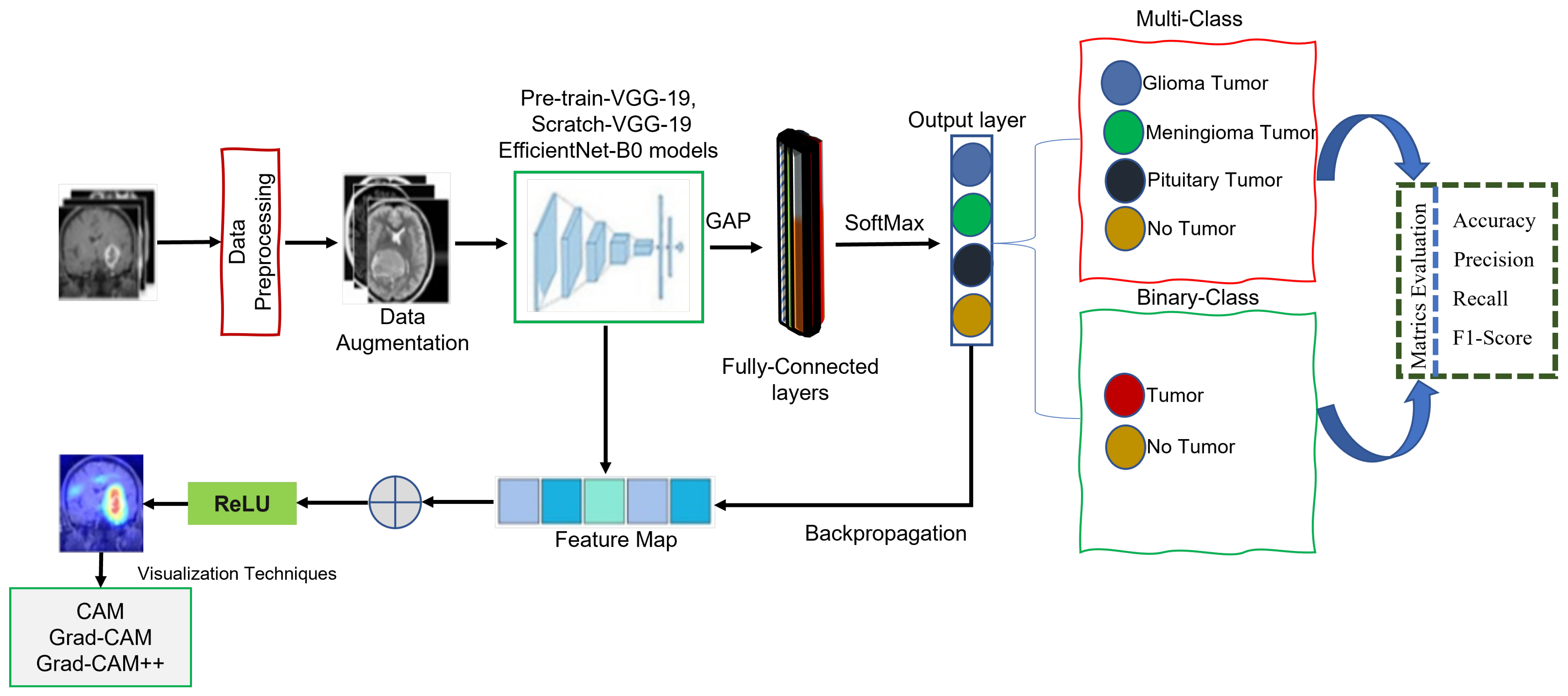
• We present a novel lightweight class-discriminative localization approach employing CAM, Grad-CAM, and Grad-CAM++ on pre-trained VGG-19, scratch VGG-19, and the EfficientNet model. This approach enhances the visual interpretability for multi-class and binary-class brain MRI tumor classification without architecture changes. The effectiveness of this approach was assessed by heatmap localization and model fidelity while maintaining a high performance.
• The proposed framework models were evaluated based on precision, recall, F1-score, accuracy, and heatmap results. We recommend the best model for both classification and localization.
• We perform CAM, Grad-CAM, and Grad-CAM++ evaluations to provide humans with understandable justifications for BT-MRI images with multi-class and binary-class architectures.
• We evaluate the performance and applicability of the proposed method in practical settings using cross-dataset.

This study employs a DL model to classify BT MRI images into multiple binary classes. Moreover, this approach visualizes the critical regions of the MR image involved in the prediction process. This study explicates the black box structure of the DL model and promotes its adoption throughout the healthcare sector. The remainder of this paper is organized as follows. Section 2 covers related work and Section 3 describes the methodology proposed in this study. Section 4 presents the numerical values obtained during the training phase of the classifier and the outcomes of the CAM, Grad-CAM, and Grad-CAM++. Section 5 provides details on the ablation study. The conclusions of this paper are discussed in Section 6.

2. Related Works

Several studies on the classification of BT-MRI images using CNN [37,38,39,40,41], pre-trained CNN models using TL [42,43,44], and tumor, polyp, and ulcer detection using a cascade approach [45] have been reported with remarkable results. However, these models lack explainability [21,22,31,46]. Although many XDL methods have been proposed for natural image problems [47,48,49], relatively less attention has been paid to model explainability in the context of brain imaging applications [19,50]. Consequently, the lack of interpretability in the models has been a concern for radiologists and healthcare professionals that find the black-box nature of the models inadequate for their needs. However, the development of XDL frameworks can advance neuroscientific research and healthcare by providing transparent and interpretable models. For this purpose, a fast and efficient multi-classification BT and localization framework using an XDL model has to be developed. An explainable framework is required to explain why particular predictions were made [51]. Many researchers have applied attribution-based explainability approaches to interpret DL [52]. In attribution-based techniques for medical images, multiple methods, such as saliency maps [53], activation maps [54], CAM [55], Grad-CAM [56], Gradient [57], and shapely additive explanations, are used [58]. The adoption of CAMs in diverse applications has recently seen the emergence of CNN-based algorithms [55,56,59,60,61,62,63,64].

The Grad-CAM technique [56] has recently been proposed to visualize essential features from the input image conserved by the CNN layers for classification. Grad-CAM has been used in various disciplines; however, it is preferred by the health sector. An extension of Grad-CAM, segmented-Grad-CAM, which enables the creation of heat maps that show the relevance of specific pixels or regions within the input images for semantic segmentation, has been proposed [63]. It generates heatmaps that indicate the relevance of certain pixels or regions within the input images for segmentation. In [64], class-selective relevance mapping (CRM), CAM, and Grad-CAM approaches were presented for the visual interpretation of different medical imaging modalities (i.e., abdomen CT, brain MRI, and chest X-ray) to clarify the prediction of the CNN-based DL model. Yang and Ranka enhanced the Grad-CAM approach to provide a 3D heatmap to visually explain and categorize cases of Alzheimer’s disease [65]. These techniques have seldom been employed for binary tumor localization [66] and are not used for multi-class BT MRI localization for model explainability. However, they are often used to interpret classification judgments [52]. In [67], a modified version of the ResNet-152 model was introduced to identify cutaneous tumors. The performance of the model was comparable with that of 16 dermatologists, and Grad-CAM was used to enhance the interpretability of the model. The success of an algorithm is significant. However, to improve the performance of explainable models, a method has to be developed for evaluating the effectiveness of an explanation [68]. In [69], deep neural networks (particularly InceptionV3 and DenseNet121) were used to generate saliency maps for chest X-ray images. They then evaluated the effectiveness of these maps by measuring the degree of overlap between the maps and human-annotated ground truths. The maps generated by these models were found to have a high degree of overlap with human annotations, indicating their potential usefulness in explainable AI in medical imaging. Interestingly, the study reported in [70] identified the improved indicators via regions (XRAI) as an effective method for generating explanations for DL models. The various DL and XDL methods proposed for the automatic classification and localization of tumors are summarized in

Table 1. Summarized related works on the classification and localization of BT.

Refs.	Method	Classification	Mode of Explanation
[71]	Feedforward neural network and DWT	Binary-class classification	Not used
[72]	CNN	Three-class BT classification	Not used
[73]	Multiscale CNN (MSCNN)	Four-class BT Classification	Not used
[74]	Multi-pathway CNN	Three-class BT classification	Not used
[75]	CNN	Multi-class brain tumor Classification	Not used
[76]	CNN with Grad-CAM	X-ray breast cancer mammogram image	Heatmap
[77]	CNN	Chest X-ray image	Heatmap
[78]	CNN	Multiple sclerosis MRI image	Heatmap

.

Table 1 shows the related approaches discussed in [76,77,78]. These studies evaluated the performances of various CNN-based classifiers on medical images and compared their characteristics by generating heatmaps. Based on these studies, Grad-CAM exhibits the most accurate localization, which is desirable for heatmaps. A localized heatmap makes it easier to identify the features that significantly contribute to the CNN classification results. Unlike the feature maps of convolutional layers, these heatmaps show the hierarchy of the importance of locations in the feature maps that contribute to classification.

3. Materials and Methods

This study aims to develop an XDL model as a promising method for categorizing and localizing multi-class and binary-class brain MRI images. The goal was to provide an autonomous system for radiologists or neurologists using CAM, Grad-CAM, and Grad-CAM++ techniques, thus enabling the accurate and efficient classification and localization of brain abnormalities. Grad-CAM has proven its ability to interpret complex neural networks, which are commonly referred to as black box models because of their complexity. The proposed method consists of the four following steps. First, the MRI dataset was prepared by pre-processing the MRI images (as discussed in Section 3.2) and utilizing data augmentation techniques to expand the MRI dataset Section 3.3). Second, three XDL models were developed for deep feature representations (as discussed in Section 3.4 and Section 3.5) based on the pre-processed MRI images. Third, the outputs of the three XDL models, pre-trained-VGG-19, scratch-VGG-19, and EfficientNet models were stacked to perform BT classification using the global average pooling (GAP) and fully connected layers, followed by a SoftMax function. Finally, CAM, Grad-CAM, and Grad-CAM++ approach was used to generate heatmaps highlighting the tumor areas of the MRI images that were most relevant to the CNN model’s predictions. This technique provides visual explanations of the model’s decision-making process, enabling radiologists or neurologists to understand the features that contribute to the model’s predictions better. Figure 1 illustrates the general process of the proposed method.

3.1. Dataset

Two publicly available open source MRI datasets were used in the experiments. The first dataset, which we obtained from the Kaggle website [79], represented the brain MRI-4C dataset. The brain MRI-4C dataset includes four types of MRI images (glioma, meningioma, pituitary, and no tumor), as shown in Figure 2. The details of this dataset are listed in

Table 2. Details of the brain MRI-4C dataset.

Tumor Type	No of MRI Images	MRI Views
Glioma tumor	926	Axial, coronal, sagittal
Meningioma tumor	937	Axial, coronal, sagittal
Pituitary tumor	901	Axial, coronal, sagittal
No tumor	501
Total number of images	3265

. The second dataset, the MRI-2C dataset, was obtained from Kaggle [80]. The MRI-2C dataset used in this study comprised two classes of MR images: tumor and normal, as illustrated in Figure 3. The details of this dataset are listed in

Table 3. Details of brain MRI-2C dataset.

Tumor Type	No of MRI Images	MRI Views
Tumor	1500	Axial, coronal, sagittal
Normal	1500
Total number of images	3000

. The MRI datasets used in this study include three different views: axial, coronal, and sagittal, as shown in Figure 4.

3.2. Data Pre-Processing

Data pre-processing is crucial in image analysis because brain MRI datasets typically contain extraneous spaces, regions, noise, and missing values that can negatively affect the classifier’s performance. Therefore, unwanted regions and noise have to be removed from MRI images. We adopted a cropping approach involving the computation of extreme points and contours [81]. Figure 5 shows the extreme-point calculation for the cropped images. To initiate the pre-processing, we loaded the MRI images from the BT dataset. The RGB images were converted to grayscale, followed by thresholding to create binary images. Furthermore, we employed dilation and erosion processes to reduce the small noise areas. A threshold image was used to locate the contour, and the largest contour was selected to determine the extreme points (extreme right, extreme left, extreme top, and extreme bottom). The image was then cropped using this information. The MRI images underwent min-max normalization before inputting into the proposed model according to Equation (1).

$$I_{normalize}(x,y)=\frac{I_{original}(x,y)-P_{min}}{P_{max}-P_{min}}$$

(1)

where $I_{normalize}(x,y)$ represents the normalized pixel value, and $I_{original}(x,y)$ represents the original pixel value at the same position. The maximum and minimum pixel values of the MRI image are denoted as $P_{max}$ and $P_{min}$, respectively. For intensity normalization, intensity values were adjusted to an interval of $[0,1]$ and then the image size was reduced to 224 × 224 before being passed to the model. This normalization step accelerates the learning process and eliminates memory problems during the network training. For this experiment, the two datasets were sorted into various categories: training, validation, and testing. The specific MRI datasets used for each category are listed in

Table 4. Brain MRI dataset used for the training, validation, and testing phases.

Brain MRI Dataset	Training	Validation	Testing	Total
MRI-4C dataset	2613	326	326	3265
MRI-2C dataset	2400	300	300	3000

.

3.3. Data Augmentation

MRI image augmentation refers to the process of artificially increasing a dataset of MRI images. The process typically involves rotating, scaling, flipping, and translating existing MRI images in the dataset, as shown in Figure 6. Data augmentation enhances the diversity of the dataset to prevent overfitting and improve the performance of the proposed model. Different augmentation procedures were used to build a new training dataset. Initially, we had the 3265 MRI-4C and 3000 MRI-2C datasets. Through augmentation, the MRI datasets increased to 6410 for MRI-4C and 5600 for MRI-2C. Different techniques were used to augment the brain MRI datasets, as listed in

Table 5. Brain MRI data augmentation steps.

Parameters	Values
Horizontal flip	True
Vertical flip	True
Range scale	True
Zoom range	[0.1, 1.0]
Width shift range	0.2
Height shift range	0.2
Shear range	0.2
Brightness range	[0.2, 1.0]
Random rotation	[0–90]

.

Table 6. Training dataset with and without augmentation.

Brain MRI Dataset	Without Augmentation	Augmented Data
MRI-4C dataset	3265	6410
MRI-2C dataset	3000	5600

shows that the augmented MRI images were almost twice those of the original images.

3.4. Pre-Trained VGG-19

In this study, a deep CNN model and VGG-19 [82] was used as a TL. The proposed system was trained using the ImageNet dataset [83]. VGG-19 has 19 layers, including 16 convolutional layers, 5 using max-pooling layers, 3 fully connected layers, and 1 one SoftMax layer. VGG-19 is an improvement over its predecessor, AlexNet [84], and has been found to outperform other models in the VGG series. TL [85] was used to effectively utilize the available resources while adhering to predefined parameters, with a pre-trained-VGG-19 model used for this study. The workflow of the pre-trained-VGG-19 model, as depicted in Figure 7, involves four main components. First, the pre-processed MRI images (discussed in Section 3.2) were input and subjected to data augmentation techniques (discussed in Section 3.3) in the initial step. The second component involves VGG-19 pre-trained CNN layers with 16 convolutional layers, followed by a rectified linear unit (ReLU) and five max-pooling layers. The input for this part of the model consisted of pre-processed MRI images with dimensions of 224 × 224. All layers in this part cannot use ImageNet weights; therefore, they cannot be trained. The layers were frozen, enabling the model to optimize its weights on the dataset and incorporate filters from the VGG-19 model to extract relevant features. To reduce the required computational resources, the dimensionality of the data was decreased using maxpooling techniques. The ReLU activation function was utilized to introduce nonlinearity into the model, thereby improving the classification performance while minimizing the computation time. Following feature extraction using multiple convolutional layers, ReLU, and max pooling, the resulting images were transformed into a (7 × 7 × 512) format. Third, the extracted features were input into the classification. The model presented in this study incorporates GAP layers, which are followed by a fully connected layer during the classification phase. The GAP layer compresses the multi-dimensional feature map into a one-dimensional (1D) feature vector. Utilizing the GAP layer avoids overfitting on this layer by not requiring parameter optimization and consumes less computation time than the scratch-VGG-19 model. The fully connected layer consists of 1024 filters, and 0.25% of the input neurons were dropped to reduce overfitting and improve the model performance. Dropout [86] was implemented to address the overfitting issue. The SoftMax function was employed to obtain the multi-class and binary-class BT classification results.

Finally, the heatmap techniques [56] were used to identify the tumor region in the brain MRI and interpret the predictions of the VGG-19 model (discussed in Section 4.4).

Global Average Pooling

In this study, both pre-trained and scratch VGG-19 models were employed for deep feature extraction. The resulting feature vectors are independently reduced using a two-dimensional (2D) GAP layer. The pooling layer was utilized to either reduce the size of the feature map or emphasize particular features. To achieve this, the GAP layer used the output data from the convolutional layer as input. It applied an average pooling (AP) to the entire feature map to generate a single output value for each feature map. Consequently, the spatial information was discarded, resulting in a 1D vector with a depth equal to the number of feature maps. In contrast to conventional AP, a sliding window was applied to each feature map to compute the average values for the non-overlapping sub-regions. This output feature map reduces the spatial dimension, but the depth is preserved. In this study, we used the GAP technique to address the issue of overfitting by compressing multi-dimensional feature maps into one-dimensional vectors. This approach significantly reduces the number of parameters required for the model and improves the computational efficiency of the network. Moreover, the GAP layer reduces the dimensionality of the data by averaging all h × w values, resulting in a feature map of size 1 × 1 × d, where d represents the number of filters. This process is illustrated in Figure 8, which illustrates the GAP operation. This technique can improve the model performance and accuracy in classifying BT by only extracting the most relevant features from the input data.

3.5. Scratch VGG-19

The scratch VGG-19 model was trained on an MRI brain dataset without utilizing pre-trained network weights. This was performed to compare the performance of the pre-trained-VGG-19 and EfficientNet models, which had already been trained using the ImageNet dataset [83]. The model also utilized CAM, Grad-CAM, and Grad-CAM++ techniques for interpretation. The scratch-VGG-19-Grad-CAM model is composed of several parts, including the input of MR images, pre-processing (discussed in Section 3.2), data augmentation (discussed in Section 3.3), feature representation, the classification of BT MRI images, and model explanation. The workflow of the proposed model is illustrated in Figure 9. The model uses a 224 × 224 MRI image as the input and data processing and augmentation techniques. The feature representation block in our model comprises convolutional and ReLU layers preceded by maxpooling layers. Following the feature extraction layer, a GAP layer was applied (as discussed in Section Global Average Pooling). The output from the GAP layer was then fed into a fully connected layer for classification. For classification, a dense layer with 1024 neurons was used, followed by a dropout layer. The SoftMax activation function was applied to classify the output image into one of the BT classes. This activation function is suitable for multi-class and binary-class classification tasks.

We evaluated the performance of the model based on various metrics (i.e., accuracy, precision, recall, and F1 score). By assessing these metrics, we can determine the effectiveness of the proposed model and make necessary adjustments to improve its performance. Additionally, we utilized the CAM, Grad-CAM, and Grad-CAM++ approach for multi-class and binary-class tumor localization (as discussed in Section 3.7) to compare the heatmap results with the pre-trained-VGG-19 and EfficientNet models.

3.6. EfficientNet-B0

A novel method for CNNs was proposed by Tan and Le (2019) [87] by uniformly scaling dimensions, including depth, width, and resolution. A specific architecture within the EfficientNet family is EfficientNet B0, whose detailed structure is depicted in Figure 10. It displays robust performance on ImageNet, and EfficientNet-B0 effectively transfers to other datasets. A TL method, especially prevalent in conjunction with DL models, involves training a CNN on a given dataset to extract features, enhancing predictive accuracy. Regardless, there are some challenges to collecting an enormous amount of data, and reliability issues arise when the data are incomplete. These issues are addressed using TL, as illustrated in Figure 10.

Through TL, a model can sustain optimal parameters based on the training process on a popular dataset like ImageNet. As a result, the learned features are re-used in the following learning task, which enhances the overall model accuracy. A TL approach is employed in this study for EfficientNet-B0 trained on ImageNet, as presented in Figure 10.

In the proposed architecture, we illustrate EfficientNet-B0 by leveraging the mobile-inverted bottleneck (MBConv) layer suggested by Sandler et al. [88,89] as the network’s main building block. However, at the end of the architecture, the output features of the pre-trained EfficientNet will be fed into our proposed layers: GAP, Dense, BN, and SoftMax activation functions. A dropout layer is incorporated with a regularization technique to mitigate overfitting during training. Using the GAP layer, we can reduce the activation size while maintaining performance. Although the dense layer is connected deeply, it receives input from all neurons from its preceding layer. Through the BN layer, the overall dimensions are normalized by evaluating the mean and variance. We adopted SoftMax as a final classifier, making the architecture more effective at classification.

Finally, we incorporated visualization techniques into our model, including CAM, Grad-CAM, and Grad-CAM++. This enhances the interpretability and transparency of the model by allowing qualitative comparisons between the inputs and predictions. As a result, it provides a valuable insight into the features that influence the model’s decision-making process.

3.7. Model Explainability

Modern DL frameworks, characterized by intricate models with millions of parameters, often face challenges in interpretation. To address this issue and enhance interpretability, techniques such as CAM, Grad-CAM, and Grad-CAM++ have been introduced. These methods aim to provide insights into the decision-making processes of Convolutional Neural Networks (CNNs).

CAM generates a class-discriminative localization map, $L_{CAM}^c$, using feature maps $A^k$ from the final convolutional layer and weights $W_k^c$ obtained through GAP.

$$L_{\mathrm{CAM}}^c=\sum _k{w}_k^c{A}_k$$

(2)

The Equation (2), represents the CAM for a specific class c in the context of a CNN.

Grad-CAM is introduced as an extension of CAM for CNNs [55]. It serves as a valuable tool for localizing discriminative attributes and illuminating object regions crucial for a CNN’s decision-making process. Unlike CAM, Grad-CAM incorporates gradient information, making it applicable to any CNN-based model without altering its architecture [56]. The Grad-CAM method identifies specific regions in the input image vital for the classifier’s decision, utilizing spatial information stored in convolutional layers. This targeted interpretation enables researchers to gain a deeper understanding of model predictions and facilitates performance optimization.

Grad-CAM generates a class-discriminative localization map, $L_{Grad-CAM}^c$, for convolutional layer of size i,j, using gradient information from feature maps ($A^k$) of the final convolutional layer [56]. Equation (3) represents the class-discriminative localization map of class c.

$$L_{Grad-CAM}^c\in R^{i\times j}$$

(3)

This is calculated for feature map activation $A^k$ and the classification score $y^c$ for class c, propagated back to the selected convolutional layer. The significant weights $W_k^c$, were computed by GAP as the gradient to the final convolutional layer according to Equation (4).

$$W_k^c=\frac{1}{z}\sum _m\sum _n\frac{\delta y^c}{\delta A_{mn}^k}$$

(4)

In Equation (4), the values of $W_k^c$ represent the importance or weightage of the feature map k for target class c. The sum of $m,n$ represents the GAP operation, and z is a constant (number of pixels in the activation map). The partial derivative represents the gradient computed through backpropagation. Subsequently, a Grad-CAM heat map was generated by computing a weighted combination of feature maps, followed by the ReLU activation function, as shown in Equation (5).

$$L_{Grad-CAM}^c=ReLU\left(\sum _k{W}_k^c{A}^k\right)$$

(5)

In Equation (5), $ReLU$ nonlinearity is only used to evaluate the pixels that have a positive impact on the target class score [56].

For Grad-CAM++, it further refines weights computation by considering second-order derivatives. The Grad-CAM++ localization map is define as:

$$L_{\mathrm{Grad}-\mathrm{CAM}++}^c=\mathrm{ReLU}\left(\sum _k{\alpha }_k{W}_k^c{A}^k\right)$$

(6)

In Equation (6), ${\alpha }_k$ represents scalar weights computed from second-order gradients, further enhancing the accuracy of the localization heat map. These equations collectively illustrate the advancement from CAM to Grad-CAM and Grad-CAM++, underscoring the increased sophistication in capturing and visualizing critical regions that significantly influence CNN decision-making processes.

4. Experimental Results and Analysis

Brain MRI was used to assess patients with BT. With two independent datasets (BT-MRI-4C and BT-MRI-2C), we performed multi-class and binary-class BT classification and localization tasks. We used the pre-trained-VGG-19, scratch-VGG-19, and EfficientNet models to correctly identify patients with tumors and those that were healthy. The proposed methods were trained with ReLU activation function (AF) with Adam optimizer to classify multi-class and binary-class BT from MRI images. Tables 8 and 9 provide the numerical analyses of the proposed architectures using metrics (precision, recall, F1-score, and accuracy) values. The bold values represent the best results.

Finally, we visualized the explainability of the model using the CAM, Grad-CAM, and Grad-CAM++ methods for the BT-MRI-4C and BT-MRI-2C datasets, which are shown in Figures 19–21 and 23.

4.1. Hyperparameter Tuning

The main objective of this task was to develop a highly efficient model for the classification of brain MRI images into multiple binary classes. Hyperparameter tuning involves the selection of the optimal values for the DL or ML models. These parameters are not learned from the data, but are set before the training begins. Hyperparameter tuning improves the model performance and designs an optimal multi-class and binary-class classification model for brain MRIs. During the experiments, we considered several parameters for hyperparameter tuning (i.e., epochs, dropout rate, activation function, batch size, and learning rate (LR)). After several trials, we adjusted the LR, batch size, regularization factor, dropout rate, and optimizer to obtain optimal results.

Table 7. Hyperparameters for the proposed models.

Sr. No.	Hyperparameters	Pre-Trained-VGG-19	Scratch-VGG-19
1	Number of epochs	30	30
2	Batch size	32	32
3	Image size	224 × 224	224 × 224
4	Optimizers	Adam, RMSprop	Adam, RMSprop
5	Activation function	SoftMax, ReLU	SoftMax, ReLU
6	Learning rate	0.0001	0.0001
7	Dropout rate	0.25	0.25

lists the hyperparameters for model training.

4.2. Classification Performance on the BT-MRI-4C and BT-MRI-2C Datasets

This study assessed the classification performance of the BT-MRI-4C and BT-MRI-2C datasets using three DL models: pre-trained-VGG-19, scratch-VGG-19, and EfficientNet. This evaluation was based on the key performance metrics such as precision, recall, F1-score, and accuracy, whilst the explainability results are discussed in Section 4.4).

This evaluation covered multi-class and binary-class prediction tasks involving fine-tuning hyperparameters such as epochs, dropout rate, activation function (ReLU), batch size, and learning rate (LR). Notably, for the BT-MRI-4C dataset, the pre-trained-VGG-19 model gives the highest performance metrics, achieving precision, recall, F1-score, and the accuracy of 99.89%, 99.72%, 99.81%, and 99.92%, respectively, outperforming the scratch-VGG-19 and EfficientNet models, as shown in

Table 8. Performance comparison of the proposed DL models on BT-MRI-4C and BT-MRI-2C datasets.

DL Model	Precision (%)	Recall (%)	F1-Score (%)	Accuracy (%)
Pre-trained-VGG-19 (BT-MRI-4C)	99.89	99.72	99.81	99.92
Scratch-VGG-19 (BT-MRI-4C)	97.69	98.95	98.39	98.94
EfficientNet (BT-MRI-4C)	99.51	98.69	99.74	99.81
Pre-trained-VGG-19 (BT-MRI-2C)	98.59	99.32	98.99	99.85
Scratch-VGG-19 (BT-MRI-2C)	95.71	95.19	96.09	96.86
EfficientNet (BT-MRI-2C)	98.01	99.06	98.81	98.65

.

This study extended to the BT-MRI-2C dataset, aiming to develop an efficient model for binary-class classification using the same configuration as BT-MRI-4C classification. The proposed models, pre-trained-VGG-19, scratch-VGG-19, and EfficientNet, were tested for binary-class classification. The pre-trained-VGG-19 model outshone the others, achieving a precision, recall, F1-score, and accuracy of 98.59%, 99.32%, 98.99%, and 99.85%, respectively, as listed in Table 8. Detailed class-wise classification metrics results in

Table 9. Class-wise metrics evaluation for both the BT-MRI-4C and BT-MRI-2C datasets using the pre-train and scratch models.

DL Model	Tumor Class	Precision (%)	Recall (%)	F1-Score (%)
Pre-trained-VGG-19 (BT-MRI-4C)	Glioma	100	99.89	100
	Meningioma	96.0	99.92	98.59
	Pituitary	99.8	100	99.91
	No tumor	100	100	100
Scratch-VGG-19 (BT-MRI-4C)	Glioma	96.0	94.00	93.00
	Meningioma	79.0	96.51	92.97
	Pituitary	88.0	92.80	89.71
	No tumor	98.0	97.00	95.68
EfficientNet (BT-MRI-4C)	Glioma	100	98.88	99.78
	Meningioma	95.00	98.10	98.63
	Pituitary	97.59	99.35	98.89
	No tumor	99.90	100	99.73
Pre-trained-VGG-19 (BT-MRI-2C)	Tumor	99.89	99.72	98.74
	Normal	100	98.39	99.40
EfficientNet (BT-MRI-2C)	Tumor	99.70	98.00	97.75
	Normal	99.79	99.10	97.38

further affirming the superiority of the pre-trained-VGG-19 model over scratch-VGG-19 and EfficientNet for both datasets.

The accuracy and loss curves are crucial for analyzing the performance of the DL models. In this experiment, we used these curves to evaluate the proposed DL models, particularly the pre-trained-VGG-19, scratch-VGG-19, and EfficientNet models, on the multi-class and binary-class BT-MRI datasets using the configuration described in Table 7. The performance of the model during training was evaluated by analyzing the training accuracy, training loss, validation accuracy, and validation loss, as shown in Figure 11, Figure 12, Figure 13 and Figure 14. The Figure 11a, Figure 12a, Figure 13a and Figure 14a show that the proposed pre-trained-VGG-19 had good convergence and minimal training and validation losses while achieving the best accuracy for both the BT-MRI-4C and BT-MRI-2C datasets.

4.3. Validation of Model Performance on a Cross-Dataset

Here, we evaluate the performance of the proposed DL models on two different unseen BT-MR image datasets obtained from Kaggle [90]. We aimed to quantify the classification accuracy of the models and assess their ability to generalize unseen data.

For the first task, we collected a dataset of 391 MRI images, consisting of 111 images of gliomas, 80 images of meningiomas, 90 images of no tumors, and 110 images of pituitary tumors. For the second task, we used a dataset of 131 MR images, consisting of 30 images of gliomas, 29 images of meningiomas, 32 images of no tumors, and 40 images of pituitary tumors. We compared the performance of the TL approach with that of the scratch model, and the results are presented in

Table 10. Class-wise classification report of cross-dataset for pre-trained-VGG-19 model test set 1.

Tumor Type	Precision	Recall	F1-Score
Glioma tumor	1.00	1.00	1.00
Meningioma tumor	1.00	1.00	1.00
Pituitary tumor	1.00	1.00	1.00
No tumor	1.00	1.00	1.00
Average (%)	100	100	100

,

Table 11. Class-wise classification report of the cross-dataset for pre-trained-VGG-19 model test set 2.

Tumor Type	Precision	Recall	F1-Score
Glioma tumor	0.97	1.00	0.98
Meningioma tumor	0.96	0.90	0.93
Pituitary tumor	1.00	1.00	1.00
No tumor	0.97	0.97	0.97
Average (%)	97.5	96.75	97.00

,

Table 12. Class-wise classification report of the cross-dataset for scratch VGG-19 model test set 1.

Tumor Type	Precision	Recall	F1-Score
Glioma tumor	0.92	0.97	0.95
Meningioma tumor	0.94	0.96	0.95
Pituitary tumor	1.00	0.94	0.97
No tumor	1.00	0.99	0.99
Average (%)	96.5	96.5	96.5

,

Table 13. Class-wise classification report of cross-dataset for the scratch VGG-19 model test set 2.

Tumor Type	Precision	Recall	F1-Score
Glioma tumor	0.71	0.97	0.82
Meningioma tumor	0.95	0.66	0.78
Pituitary tumor	1.00	0.95	0.97
No tumor	1.00	1.00	1.00
Average (%)	91.5	89.5	89.25

,

Table 14. Class-wise classification report of cross-dataset for EfficientNet model test set 1.

Tumor Type	Precision	Recall	F1-Score
Glioma tumor	0.98	0.98	0.98
Meningioma tumor	0.94	0.98	0.96
Pituitary tumor	0.99	0.963	0.97
No tumor	1.00	0.98	0.99
Average (%)	97.8	98.05	97.92

and

Table 15. Class-wise classification report of cross-dataset for EfficientNet model test set 2.

Tumor Type	Precision	Recall	F1-Score
Glioma tumor	0.88	1.00	0.93
Meningioma tumor	0.92	0.89	0.91
Pituitary tumor	1.00	0.85	0.91
No tumor	0.91	1.00	0.95
Average (%)	93.13	93.66	93.09

, Figure 15, Figure 16 and Figure 17. This performed better in classifying the multi-class BT from the unseen dataset compared to the scratch-VGG-19 and EfficientNet model. This demonstrates the effectiveness of feature representation and the usefulness of TL. We evaluated the model performance using a confusion matrix to analyze the true positive, true negative, false positive, and false negative rates. We assessed the predictive strength of the model [56] using performance metrics such as precision, recall, and F1-score. These metrics provide a more detailed analysis of the model performance and help identify areas where the model may need improvement.

Precision: Ratio of true positive predictions to the sum of true positives and false negatives.

$$Precision=\frac{TP}{(TP+FP)}$$

(7)

Recall: Ratio of true positive predictions to the sum of true positives and false negatives.

$$Recall=\frac{TP}{(TP+FN)}$$

(8)

F1-score: A harmonic mean is taken to combine precision and recall.

$$F1-Score=2\times \frac{Precision\times Recall}{Precision+Recall}$$

(9)

$TP$, $FP$, and $FN$ denote true positive, false positive, and false negative, respectively. The evaluation results are presented in Table 10 and Table 11, demonstrating that the pre-trained VGG-19 model outperforms the Scratch-VGG-19 and EfficientNet model in terms of precision, recall, F1-score, and average scores. This contrasts with the findings presented in Table 12, Table 13, Table 14 and Table 15. This demonstrates the effectiveness of TL in improving the model performance. The confusion matrix provides insights into the number of correctly and incorrectly classified images using the model. Figure 15, Figure 16 and Figure 17 present a detailed analysis of each model’s correct and incorrect classifications on both cross-datasets. The results were deemed acceptable based on a confusion matrix. The pre-trained-VGG-19 model outperforms the scratch-VGG-19 and EfficientNet model. Figure 15a shows that the pre-trained-VGG-19 model perfectly classified each class without misclassification for the first task on the cross-dataset. As shown in Figure 15b, our proposed model also performed well for all classes except two meningiomas and one no-tumor class image, which were misclassified for the second cross-dataset task. Compared with the scratch-VGG-19 and EfficientNet model, the ratio of misclassification in both datasets for the scratch-VGG-19 and EfficientNet model are higher as compared to the pre-trained-VGG-19 model. Figure 16a,b and Figure 17a,b show the scratch-VGG-19 and EfficientNet model results for both the cross-dataset tasks.

To evaluate the effectiveness of the pre-trained-VGG-19 model, we tested the proposed models on the MRI-2C dataset and compared the performance with scratch-VGG-19 and EfficientNet models. The classification results are summarized in

Table 16. The class-wise metrics evaluation of the performances of the proposed model for BT-MRI-2C datasets The bold method shows the highest performance.

DL Model	Tumor Class	Precision (%)	Recall (%)	F1-Score (%)
Pre-trained-VGG-19 (BT-MRI-2C)	Tumor	100	96.00	98.00
	No tumor	96.00	100	98.00
Scratch-VGG-19 (BT-MRI-2C)	Tumor	98.10	91.96	94.93
	No tumor	91.59	98.00	94.69
EfficientNet (BT-MRI-2C)	Tumor	99.46	98.20	97.32
	No tumor	98.02	96.12	97.06

based on various metrics. The pre-trained-VGG-19 model gives the highest results for the BT-MRI-2C dataset, achieving 100% precision, 96% recall, and a 98% F1-score. Notably, for the tumor class, the pre-trained-VGG-19 model achieved significantly higher precision and F1-scores (100% and 98.00%, respectively) compared to the scratch-VGG-19 and EfficientNet models as shown in Table 16. Table 16 presents the class-wise performance of the models, demonstrating that the pre-trained-VGG-19 model for binary classification achieved the most accurate results when calculating the precision, recall, and F1-score.

Furthermore, Figure 18a–c shows the confusion matrix for the results of the suggested models. Figure 18a shows the proposed pre-trained-VGG-19 model, which correctly classified 108 out of 112 patients with a tumor, and four instances where the model incorrectly classified a sample as not having a tumor. Additionally, there were 100 instances where the model correctly classified the sample as healthy and no instances where the model incorrectly classified a healthy sample as having a tumor. The model performed well overall, with a high number of correct predictions for both tumor and non-tumor samples compared to the scratch-VGG-19 and EfficientNet models, as shown in Figure 18b,c.

4.4. Model Explainability Results

CAM, Grad-CAM, and Grad-CAM++ were used to clearly explain the predictions when dealing with model explainability. It was tested and found to produce better visualization results using the proposed medical image classification model. Figure 19, Figure 20, Figure 21, Figure 22 and Figure 23 show the visualization results produced by our proposed models using heatmap methods for multi-class and binary-class BT MRI images. We can differentiate between the original images and heatmaps created using the CAM, Grad-CAM, and Grad-CAM++ methods and the visualizations produced by overlaying the original image on the heatmap. In Figure 19 and Figure 21, Figure 22 and Figure 23, the red circle indicates the ground truth for the tumor area, whereas the green circle represents the predicted heatmap generated by the proposed models for the multi-class and binary-class BT MRI datasets. Similarly, in Figure 20, the red circle represents the ground truth of the tumor area, whereas the yellow circle represents the predicted heatmaps for the scratch-VGG-19 model.

The heatmap technique uses a color range from yellow to dark red, where yellow indicates low-contribution regions and dark red indicates high-contribution regions, as shown in Figure 19, Figure 20, Figure 21, Figure 22 and Figure 23. These figures demonstrate the MRI regions significantly contributing to the predicted classification results, making the model more interpretable for humans. Therefore, anyone can understand which regions of the MRI are used for classification. When pixel-wise correctness is not required, heatmaps can serve as alternatives for segmentation. The labeling and training MRI datasets for segmentation using BT are computationally intensive. Therefore, heatmaps can be an alternative and a trade-off between accuracy and resource requirements. In Figure 19, Figure 20 and Figure 21, GI-T, Mi-T, and Pi-T represent the glioma, meningioma, and pituitary tumor with corresponding visualization results, respectively.

The numerical evaluation results in Table 10, Table 11, Table 12, Table 13, Table 14 and Table 15 and model explainability results in Figure 19, Figure 20, Figure 21, Figure 22 and Figure 23 show that the pre-trained-VGG-19 using Grad-CAM outperforms the scratch-VGG-19 and EfficientNet model due to its transferability knowledge of pre-trained models for multi-class as well as binary-class brain MRI image classification and localization.

Figure 22 displays a comparative analysis of the explainability results obtained from the pre-trained-VGG-19-Grad-CAM, scratch-VGG-19-Grad-CAM, and EfficientNet-Grad-CAM models. These models were evaluated using the BT-MRI-4C dataset (excluding no tumor class for localization), and the qualitative results were examined. The red boxes in Figure 22 represent the ground-truth bounding boxes, while the green boxes indicate the predicted bounding boxes generated by the proposed models. Upon visual inspection, it is evident that the pre-trained-VGG-19 using the Grad-CAM model in Figure 22a exhibits a significantly better precision for multi-class BT localization compared to the scratch-VGG-19 in Figure 22b and the EfficientNet model shown in Figure 22c for multi-class BT-MRI-4C as well as the pre-trained-VGG-19 using Grad-CAM gives better localization for the BT-MRI-2C dataset (exclude no tumor image class for localization, and only consider tumor class) as observed in Figure 23. Interestingly, the scratch-VGG-19 and EfficientNet models using CAM, Grad-CAM, and Grad-CAM++ model tend to identify non-discriminative object parts, as shown in Figure 22b,c and Figure 23.

The pre-trained-VGG-19 classification model (the most accurate) implemented via the Grad-CAM technique showed significant accuracy in multi-class and binary-class BT diagnosis prediction while demonstrating explainable capabilities. Grad-CAM can diagnose possible abnormalities in MR images (gliomas, meningiomas, and pituitary tumors) based on its ability to identify regions of interest.

4.5. Comparison with State-of-the-Art Deep Learning Models

As presented in

Table 17. Performance-based comparison of the proposed model with state-of-the-art DL models.

Ref	Method	Parameters	Dataset	Accuracy	Model Explainability
[91]	CNN,			97.60%
	SVM,	Not mentioned	Three-class	98.30%	Not used
	KNN, SoftMax			94.90%
[92]	CNN, SoftMax	Not mentioned	Three-class	97.42%	Not used
[72]	CNN, SoftMax	Not mentioned	Three-class	95.23%	Not used
[98]	VGG-16			95.9%
	DenseNet-161	Not mentioned	Three-class	98.9%	Not used
	ResNet-18			76%
[101]	GCNN	Not mentioned	Two-class	99.8%	Not used
	GCNN	Not mentioned	Three-class	97.14%	Not used
[99]	Lightweight CNN	0.59 M	Two class	98.55%	Not used
	Lightweight CNN	0.59 M	Three class	96.83%	Not used
[100]	VGG16	Not mentioned	Three-class	97.80%	Not used
	ResNet50	Not mentioned	Three-class	97.40%	Not used
[93]			Four-class	95.71%
	CNN,	Not mentioned	Three-class	97.23%	Not used
	SoftMax		Binary-class	99.83%
[66]	CNN, SoftMax	Not mentioned	Binary-class	99.33%	Grad-CAM for binary-class prediction
Our proposed model	Pre-trained-VGG-19, SoftMax	20 M	BT-MRI-4C	99.92%
	Scratch VGG-19, SoftMax	139 M	BT-MRI-4C	98.94%
	EfficientNet, SoftMax	10 M	BT-MRI-4C	99.81%
	Pre-trained-VGG-19, SoftMax	12 M	BT-MRI-2C	99.85%	CAM, Grad-CAM and Grad-CAM++ for binary and multi-class predication
	Scratch-VGG-19, SoftMax	9 M	BT-MRI-2C	96.79%
	EfficientNet, SoftMax	10 M	BT-MRI-2C	98.65%

, we compared the proposed model with existing BT and chest X-ray images classification and segmentation methods [66,72,91,92,93,94,95,96,97,98,99,100,101,102] that utilize various DL techniques. The comparison was based on the accuracy and the model explainability results using Grad-CAM. The classification accuracy of our model for the BT-MRI-4C dataset using the pre-trained-VGG-19 is 99.92%, the scratch-VGG-19 model is 98.94%, and the EfficientNet model achieves 99.81%. Similarly, for the BT-MRI-2C dataset, the proposed pre-trained-VGG-19 achieved 99.85%, scratch-VGG-19 achieved 96.79%, and EfficientNet model achieved 98.65% accuracy. Furthermore, for the chest X-ray image dataset, the proposed pre-trained-VGG-19, scratch-VGG-19, and EfficientNet models achieved an accuracy of 98.03%, 96.09%, and 97.59%. We used model explainability techniques using the CAM, Grad-CAM, and Grad-CAM++ to visualize the regions that are most relevant to a specific prediction. Thus, researchers can gain insights into how the model works and how it can be improved to increase its accuracy and performance.

Table 17 shows that our proposed model gives better classification and explainability results using CAM, Grad-CAM, and Grad-CAM++. The results of this study demonstrate the reliability of the proposed system. In [91], a CNN model with different classifiers was used for a three-class (glioma, meningioma, and pituitary tumor) MRI dataset and obtained the best accuracy of 98.30% using the K-NN classifier. However, they did not use a model-explainability study. The authors [72,92] proposed different CNN models using the SoftMax classifier for three-class classification, but they did not introduce the best prediction results. In [93], the author used an attention-guided CNN (AG-CNN) model for multi-(four-class, three-class) and binary class classification, obtaining a better recognition accuracy for the binary class, which was 99.83%, and did not obtain good recognition accuracy for either the four-class or three-class BT, which were 95.71% and 97.23%, respectively. Owing to the imbalance in the dataset, the AG-CNN model tended to be more biased toward the glioma class in the three-class and four-class datasets, resulting in poor classification. Moreover, they do not explain the model’s explainability. The authors in [66] proposed the EfficientNet-B0 CNN model for binary-class (tumor and healthy) classification, achieving an accuracy of 99.33% without data augmentation techniques. In this study, the tumor class was visualized through a heatmap using Grad-CAM techniques. This study only focused on binary classes and not on multi-class BT-MR images.

Our proposed pre-trained-VGG-19 utilizing Grad-CAM demonstrated superiority over existing methods for the multi-class and binary-class classification of the BT-MRI dataset, as evidenced by the performance evaluation. Table 17 compares our method with the existing quantitative and qualitative literature. We found our approach to be the most accurate. We believe that this study is the first to use CAM, Grad-CAM, and Grad-CAM++ to localize and classify the BT-MRI and chest X-ray images, with the model explainability making a significant contribution to the field.

5. Ablation Study

In this ablation study, we thoroughly evaluated the performance of the proposed neural network architectures: pre-trained VGG-19, scratch-VGG-19, and EfficientNet for BT-MRI-4C and BT-MRI-2C classification. As shown in

Table 18. Performance comparison of proposed models for both optimizers and evaluation matrices for the BT-MRI-4C dataset.

Model	Optimizer	Precision (%)	Recall (%)	F1-Score (%)	Accuracy (%)
Pre-trained-VGG-19	Adam	99.89	99.72	99.81	99.92
	RMSprop	99.10	98.99	99.08	99.69
Scratch-VGG-19	Adam	97.69	98.95	98.39	98.94
	RMSprop	97.57	97.09	98.99	97.09
EfficientNet	Adam	99.51	98.69	99.74	99.81
	RMSprop	98.42	98.75	98.14	99.62

and

Table 19. Performance comparison of proposed models for both optimizer and evaluation matrices for the BT-MRI-2C dataset.

Model	Optimizer	Precision (%)	Recall (%)	F1-Score (%)	Accuracy (%)
Pre-trained-VGG-19	Adam	98.59	99.32	98.99	99.85
	RMSprop	98.57	98.59	97.80	98.12
Scratch-VGG-19	Adam	96.30	95.79	96.90	96.79
	RMSprop	96.01	94.38	96.00	95.92
EfficientNet	Adam	98.01	99.06	98.81	98.65
	RMSprop	98.26	97.31	97.40	98.01

, the pre-trained-VGG-19 performance was notable across all metrics and exhibited excellent precision, recall, F1-score, and accuracy. Using pre-trained weights from ImageNet contributed to VGG-19 exceptional performance in recognizing BT patterns by providing a robust foundation. While EfficientNet did not outperform pre-trained-VGG-19 in all metrics, it showed commendable stability. Its efficient scaling strategy, balancing model size and performance, led to consistent results. It was interesting to note that the proposed models performed better with Adam compared to RMSprop as shown in Table 18 and Table 19. In terms of performance, the scratch-VGG-19 showed competitive results but slightly fell behind the pre-trained VGG-19 and EfficientNet models. It can directly learn relevant features from the BT-MRI dataset, illustrating its effectiveness without pre-existing weights.

To check the effectiveness of the proposed study, we extended our study to the Chest X-ray images dataset [103]. The pre-trained VGG-19 continued to excel, achieving 98.03% accuracy, 97.91% precision, 97.01% recall, and 96.84% F1-score, compared to the scratch-VGG-19 and EfficientNet models, as shown in

Table 20. Performance comparison of proposed models for both the optimizer and evaluation matrices for the chest X-ray dataset.

Model	Optimizer	Precision (%)	Recall (%)	F1-Score (%)	Accuracy (%)
Pre-trained-VGG-19	Adam	97.91	97.01	96.84	98.03
	RMSprop	97.11	96.85	96.21	97.09
Scratch-VGG-19	Adam	95.31	94.86	95.37	96.09
	RMSprop	95.01	94.28	95.41	95.71
EfficientNet	Adam	97.59	96.88	96.61	97.59
	RMSprop	97.15	96.08	95.97	97.53

. In light of this versatility, the pre-trained VGG-19 is suitable for many different applications in the medical imaging field. Furthermore, heatmap visualization techniques, such as Grad-CAM, were more interpretable than CAM and Grad-CAM++, as shown in Figure 24. The Grad-CAM visual explanation highlighted the most important region in the input images, allowing clinicians to gain much-needed insights into the model decisions.

6. Conclusions

In this study, we introduce an XDL model based on real-world diagnostic procedures to detect multi-class and binary-class BT-MRI images. The interpretability of models is essential in high-stack domains for DL solutions. Research on applying explainable DL for multi-class BT classification and localization was rare despite the large number of papers on binary-class BT classification and segmentation using DL and ML. Hence, in this study, we presented three DL models (pre-trained-VGG-19, scratch-VGG-19, and EfficientNet) for multi-class and binary-class BT classification and localization using CAM, Grad-CAM, and Grad-CAM++. The pre-trained-VGG-19 and EfficientNet models were used as the TL approach, whereas scratch-VGG-19 was trained from scratch for the brain MRI dataset using different optimizers (ADAM and RMSprop) and medical datasets. The proposed DL model was visualized using heatmap techniques to facilitate understanding and explanation. The experimental results demonstrated that the pre-trained-VGG-19 model utilizing the Grad-CAM technique performed better than the scratch-VGG-19 and EfficientNet model and the other cutting-edge DL techniques, both in the visual and quantitative evaluations, with improved accuracy. This indicates the efficacy of our suggested strategy and the potential for adopting DL for quick BT diagnoses using MRI images. Radiologists can use the proposed method to obtain a secondary opinion. It minimizes the calculation time and improves the accuracy. An automatic classification system can significantly reduce the diagnosis time and manpower requirements. Consequently, this was performed to minimize misclassification.

The proposed approach will be tested on various tumor imaging challenges using the transformer model in future studies. The model will be further refined and its performance enhanced through experimentation with the challenging medical imaging dataset.

References

1. Amin, J.; Sharif, M.; Yasmin, M.; Fernandes, S.L. A distinctive approach in brain tumor detection and classification using MRI. Pattern Recognit. Lett. 2020, 139, 118–127. [Google Scholar] [CrossRef]
2. Amin, J.; Sharif, M.; Yasmin, M.; Fernandes, S.L. Big data analysis for brain tumor detection: Deep convolutional neural networks. Future Gener. Comput. Syst. 2018, 87, 290–297. [Google Scholar] [CrossRef]
3. Nazir, M.; Shakil, S.; Khurshid, K. Role of deep learning in brain tumor detection and classification (2015 to 2020): A review. Comput. Med Imaging Graph. 2021, 91, 101940. [Google Scholar] [CrossRef] [PubMed]
4. Tiwari, A.; Srivastava, S.; Pant, M. Brain tumor segmentation and classification from magnetic resonance images: Review of selected methods from 2014 to 2019. Pattern Recognit. Lett. 2020, 131, 244–260. [Google Scholar] [CrossRef]
5. Mohan, G.; Subashini, M.M. MRI based medical image analysis: Survey on brain tumor grade classification. Biomed. Signal Process. Control 2018, 39, 139–161. [Google Scholar] [CrossRef]
6. Ayadi, W.; Charfi, I.; Elhamzi, W.; Atri, M. Brain tumor classification based on hybrid approach. Vis. Comput. 2022, 38, 107–117. [Google Scholar] [CrossRef]
7. Siegel, R.L.; Miller, K.D.; Wagle, N.S.; Jemal, A. Cancer statistics, 2023. CA Cancer J. Clin. 2023, 73, 17–48. [Google Scholar] [CrossRef] [PubMed]
8. Dandıl, E.; Çakıroğlu, M.; Ekşi, Z. Computer-aided diagnosis of malign and benign brain tumors on MR images. In Proceedings of the ICT Innovations 2014: World of Data, Ohrid, Macedonia, 9–12 September 2014; Springer: Cham, Switzerland, 2015; pp. 157–166. [Google Scholar]
9. Tu, L.; Luo, Z.; Wu, Y.L.; Huo, S.; Liang, X.J. Gold-based nanomaterials for the treatment of brain cancer. Cancer Biol. Med. 2021, 18, 372. [Google Scholar] [CrossRef]
10. Miner, R.C. Image-guided neurosurgery. J. Med. Imaging Radiat. Sci. 2017, 48, 328–335. [Google Scholar] [CrossRef]
11. Paul, J.; Sivarani, T. Computer aided diagnosis of brain tumor using novel classification techniques. J. Ambient. Intell. Humaniz. Comput. 2021, 12, 7499–7509. [Google Scholar] [CrossRef]
12. Abd El-Wahab, B.S.; Nasr, M.E.; Khamis, S.; Ashour, A.S. BTC-fCNN: Fast Convolution Neural Network for Multi-class Brain Tumor Classification. Health Inf. Sci. Syst. 2023, 11, 3. [Google Scholar] [CrossRef] [PubMed]
13. Khan, M.S.I.; Rahman, A.; Debnath, T.; Karim, M.R.; Nasir, M.K.; Band, S.S.; Mosavi, A.; Dehzangi, I. Accurate brain tumor detection using deep convolutional neural network. Comput. Struct. Biotechnol. J. 2022, 20, 4733–4745. [Google Scholar] [CrossRef] [PubMed]
14. Wijethilake, N.; Meedeniya, D.; Chitraranjan, C.; Perera, I.; Islam, M.; Ren, H. Glioma survival analysis empowered with data engineering—A survey. IEEE Access 2021, 9, 43168–43191. [Google Scholar] [CrossRef]
15. Yang, G.; Ye, Q.; Xia, J. Unbox the black-box for the medical explainable AI via multi-modal and multi-centre data fusion: A mini-review, two showcases and beyond. Inf. Fusion 2022, 77, 29–52. [Google Scholar] [CrossRef] [PubMed]
16. O’Mahony, N.; Campbell, S.; Carvalho, A.; Harapanahalli, S.; Hernandez, G.V.; Krpalkova, L.; Riordan, D.; Walsh, J. Deep learning vs. traditional computer vision. In Advances in Computer Vision, Proceedings of the 2019 Computer Vision Conference (CVC), Las Vegas, NV, USA, 2–3 May 2019; Springer: Cham, Switzerland, 2020; Volume 1, pp. 128–144. [Google Scholar]
17. Huang, P.; He, P.; Tian, S.; Ma, M.; Feng, P.; Xiao, H.; Mercaldo, F.; Santone, A.; Qin, J. A ViT-AMC network with adaptive model fusion and multiobjective optimization for interpretable laryngeal tumor grading from histopathological images. IEEE Trans. Med. Imaging 2022, 42, 15–28. [Google Scholar] [CrossRef] [PubMed]
18. Huang, P.; Tan, X.; Zhou, X.; Liu, S.; Mercaldo, F.; Santone, A. FABNet: Fusion attention block and transfer learning for laryngeal cancer tumor grading in P63 IHC histopathology images. IEEE J. Biomed. Health Inform. 2021, 26, 1696–1707. [Google Scholar] [CrossRef]
19. Gulum, M.A.; Trombley, C.M.; Kantardzic, M. A review of explainable deep learning cancer detection models in medical imaging. Appl. Sci. 2021, 11, 4573. [Google Scholar] [CrossRef]
20. Ahmed Salman, S.; Lian, Z.; Saleem, M.; Zhang, Y. Functional Connectivity Based Classification of ADHD Using Different Atlases. In Proceedings of the 2020 IEEE International Conference on Progress in Informatics and Computing (PIC), Shanghai, China, 18–20 December 2020; pp. 62–66. [Google Scholar] [CrossRef]
21. Shah, H.A.; Saeed, F.; Yun, S.; Park, J.H.; Paul, A.; Kang, J.M. A robust approach for brain tumor detection in magnetic resonance images using finetuned efficientnet. IEEE Access 2022, 10, 65426–65438. [Google Scholar] [CrossRef]
22. Asif, S.; Yi, W.; Ain, Q.U.; Hou, J.; Yi, T.; Si, J. Improving effectiveness of different deep transfer learning-based models for detecting brain tumors from MR images. IEEE Access 2022, 10, 34716–34730. [Google Scholar] [CrossRef]
23. Amin, J.; Sharif, M.; Gul, N.; Yasmin, M.; Shad, S.A. Brain tumor classification based on DWT fusion of MRI sequences using convolutional neural network. Pattern Recognit. Lett. 2020, 129, 115–122. [Google Scholar] [CrossRef]
24. Rehman, A.; Khan, M.A.; Saba, T.; Mehmood, Z.; Tariq, U.; Ayesha, N. Microscopic brain tumor detection and classification using 3D CNN and feature selection architecture. Microsc. Res. Tech. 2021, 84, 133–149. [Google Scholar] [CrossRef] [PubMed]
25. Wijethilake, N.; Islam, M.; Meedeniya, D.; Chitraranjan, C.; Perera, I.; Ren, H. Radiogenomics of glioblastoma: Identification of radiomics associated with molecular subtypes. In Machine Learning in Clinical Neuroimaging and Radiogenomics in Neuro-Oncology, Proceedings of the Third International Workshop, MLCN 2020, and Second International Workshop, RNO-AI 2020, Held in Conjunction with MICCAI 2020, Lima, Peru, 4–8 October 2020; Proceedings 3; Springer: Cham, Switzerland, 2020; pp. 229–239. [Google Scholar]
26. Wijethilake, N.; Meedeniya, D.; Chitraranjan, C.; Perera, I. Survival prediction and risk estimation of Glioma patients using mRNA expressions. In Proceedings of the 2020 IEEE 20th International Conference on Bioinformatics and Bioengineering (BIBE), Cincinnati, OH, USA, 26–28 October 2020; pp. 35–42. [Google Scholar]
27. Salman, S.A.; Zakir, A.; Takahashi, H. Cascaded deep graphical convolutional neural network for 2D hand pose estimation. In Proceedings of the International Workshop on Advanced Imaging Technology (IWAIT) 2023; Nakajima, M., Kim, J.G., deok Seo, K., Yamasaki, T., Guo, J.M., Lau, P.Y., Kemao, Q., Eds.; International Society for Optics and Photonics, SPIE: San Diego, CA, USA, 2023; Volume 12592, p. 1259215. [Google Scholar] [CrossRef]
28. Singh, V.K. Segmentation and Classification of Multimodal Medical Images Based on Generative Adversarial Learning and Convolutional Neural Networks. Ph.D. Thesis, Universitat Rovira i Virgili, Tarragona, Spain, 2020. [Google Scholar]
29. Abdelhafiz, D.; Yang, C.; Ammar, R.; Nabavi, S. Deep convolutional neural networks for mammography: Advances, challenges and applications. BMC Bioinform. 2019, 20, 281. [Google Scholar] [CrossRef] [PubMed]
30. Song, Y.; Rana, M.N.; Qu, J.; Liu, C. A Survey of Deep Learning Based Methods in Medical Image Processing. Curr. Signal Transduct. Ther. 2021, 16, 101–114. [Google Scholar] [CrossRef]
31. Kang, J.; Ullah, Z.; Gwak, J. Mri-based brain tumor classification using ensemble of deep features and machine learning classifiers. Sensors 2021, 21, 2222. [Google Scholar] [CrossRef] [PubMed]
32. Deepak, S.; Ameer, P. Brain tumor classification using deep CNN features via transfer learning. Comput. Biol. Med. 2019, 111, 103345. [Google Scholar] [CrossRef] [PubMed]
33. Erhan, D.; Manzagol, P.A.; Bengio, Y.; Bengio, S.; Vincent, P. The difficulty of training deep architectures and the effect of unsupervised pre-training. In Proceedings of the Artificial Intelligence and Statistics, Clearwater Beach, FL, USA, 16–18 April 2009; pp. 153–160. [Google Scholar]
34. Azizpour, H.; Sharif Razavian, A.; Sullivan, J.; Maki, A.; Carlsson, S. From generic to specific deep representations for visual recognition. In Proceedings of the IEEE Conference on Computer Vision and Pattern Recognition Workshops, Boston, MA, USA, 7–12 June 2015; pp. 36–45. [Google Scholar]
35. Penatti, O.A.; Nogueira, K.; Dos Santos, J.A. Do deep features generalize from everyday objects to remote sensing and aerial scenes domains? In Proceedings of the IEEE Conference on Computer Vision and Pattern Recognition Workshops, Boston, MA, USA, 7–12 June 2015; pp. 44–51. [Google Scholar]
36. Salman, S.A.; Zakir, A.; Takahashi, H. SDFPoseGraphNet: Spatial Deep Feature Pose Graph Network for 2D Hand Pose Estimation. Sensors 2023, 23, 9088. [Google Scholar] [CrossRef]
37. Badža, M.M.; Barjaktarović, M.Č. Classification of brain tumors from MRI images using a convolutional neural network. Appl. Sci. 2020, 10, 1999. [Google Scholar] [CrossRef]
38. Mzoughi, H.; Njeh, I.; Wali, A.; Slima, M.B.; BenHamida, A.; Mhiri, C.; Mahfoudhe, K.B. Deep multi-scale 3D convolutional neural network (CNN) for MRI gliomas brain tumor classification. J. Digit. Imaging 2020, 33, 903–915. [Google Scholar] [CrossRef]
39. Ayadi, W.; Elhamzi, W.; Charfi, I.; Atri, M. Deep CNN for brain tumor classification. Neural Process. Lett. 2021, 53, 671–700. [Google Scholar] [CrossRef]
40. Abiwinanda, N.; Hanif, M.; Hesaputra, S.T.; Handayani, A.; Mengko, T.R. Brain tumor classification using convolutional neural network. In Proceedings of the World Congress on Medical Physics and Biomedical Engineering 2018, Prague, Czech Republic, 3–8 June 2018; Springer: Cham, Switzerland, 2019; Volume 1, pp. 183–189. [Google Scholar]
41. Sultan, H.H.; Salem, N.M.; Al-Atabany, W. Multi-classification of brain tumor images using deep neural network. IEEE Access 2019, 7, 69215–69225. [Google Scholar] [CrossRef]
42. Çinar, A.; Yildirim, M. Detection of tumors on brain MRI images using the hybrid convolutional neural network architecture. Med. Hypotheses 2020, 139, 109684. [Google Scholar] [CrossRef]
43. Rehman, A.; Naz, S.; Razzak, M.I.; Akram, F.; Imran, M. A deep learning-based framework for automatic brain tumors classification using transfer learning. Circuits Syst. Signal Process. 2020, 39, 757–775. [Google Scholar] [CrossRef]
44. Mehrotra, R.; Ansari, M.; Agrawal, R.; Anand, R. A transfer learning approach for AI-based classification of brain tumors. Mach. Learn. Appl. 2020, 2, 100003. [Google Scholar] [CrossRef]
45. Rahim, T.; Usman, M.A.; Shin, S.Y. A survey on contemporary computer-aided tumor, polyp, and ulcer detection methods in wireless capsule endoscopy imaging. Comput. Med. Imaging Graph. 2020, 85, 101767. [Google Scholar] [CrossRef] [PubMed]
46. Rai, H.M.; Chatterjee, K. 2D MRI image analysis and brain tumor detection using deep learning CNN model LeU-Net. Multimed. Tools Appl. 2021, 80, 36111–36141. [Google Scholar] [CrossRef]
47. Intagorn, S.; Pinitkan, S.; Panmuang, M.; Rodmorn, C. Helmet Detection System for Motorcycle Riders with Explainable Artificial Intelligence Using Convolutional Neural Network and Grad-CAM. In Proceedings of the International Conference on Multi-disciplinary Trends in Artificial Intelligence, Hyberabad, India, 17–19 November 2022; Springer: Cham, Switzerland, 2022; pp. 40–51. [Google Scholar]
48. Dworak, D.; Baranowski, J. Adaptation of Grad-CAM method to neural network architecture for LiDAR pointcloud object detection. Energies 2022, 15, 4681. [Google Scholar] [CrossRef]
49. Lucas, M.; Lerma, M.; Furst, J.; Raicu, D. Visual explanations from deep networks via Riemann-Stieltjes integrated gradient-based localization. arXiv 2022, arXiv:2205.10900. [Google Scholar]
50. Chen, H.; Gomez, C.; Huang, C.M.; Unberath, M. Explainable medical imaging AI needs human-centered design: Guidelines and evidence from a systematic review. NPJ Digit. Med. 2022, 5, 156. [Google Scholar] [CrossRef]
51. Arrieta, A.B.; Díaz-Rodríguez, N.; Del Ser, J.; Bennetot, A.; Tabik, S.; Barbado, A.; García, S.; Gil-López, S.; Molina, D.; Benjamins, R.; et al. Explainable Artificial Intelligence (XAI): Concepts, taxonomies, opportunities and challenges toward responsible AI. Inf. Fusion 2020, 58, 82–115. [Google Scholar] [CrossRef]
52. Singh, A.; Sengupta, S.; Lakshminarayanan, V. Explainable deep learning models in medical image analysis. J. Imaging 2020, 6, 52. [Google Scholar] [CrossRef]
53. Lévy, D.; Jain, A. Breast mass classification from mammograms using deep convolutional neural networks. arXiv 2016, arXiv:1612.00542. [Google Scholar]
54. Van Molle, P.; De Strooper, M.; Verbelen, T.; Vankeirsbilck, B.; Simoens, P.; Dhoedt, B. Visualizing convolutional neural networks to improve decision support for skin lesion classification. In Understanding and Interpreting Machine Learning in Medical Image Computing Applications, Proceedings of the First International Workshops, MLCN 2018, DLF 2018, and iMIMIC 2018, Held in Conjunction with MICCAI 2018, Granada, Spain, 16–20 September 2018; Proceedings 1; Springer: Cham, Switzerland, 2018; pp. 115–123. [Google Scholar]
55. Zhou, B.; Khosla, A.; Lapedriza, A.; Oliva, A.; Torralba, A. Learning deep features for discriminative localization. In Proceedings of the IEEE Conference on Computer Vision and Pattern Recognition, Las Vegas, NV, USA, 27–30 June 2016; pp. 2921–2929. [Google Scholar]
56. Selvaraju, R.R.; Cogswell, M.; Das, A.; Vedantam, R.; Parikh, D.; Batra, D. Grad-cam: Visual explanations from deep networks via gradient-based localization. In Proceedings of the IEEE International Conference on Computer Vision, Venice, Italy, 22–29 October 2017; pp. 618–626. [Google Scholar]
57. Eitel, F.; Ritter, K.; Alzheimer’s Disease Neuroimaging Initiative (ADNI). Testing the robustness of attribution methods for convolutional neural networks in MRI-based Alzheimer’s disease classification. In Interpretability of Machine Intelligence in Medical Image Computing and Multimodal Learning for Clinical Decision Support, Proceedings of the Second International Workshop, iMIMIC 2019, and 9th International Workshop, ML-CDS 2019, Held in Conjunction with MICCAI 2019, Shenzhen, China, 17 October 2019; Proceedings 9; Springer: Cham, Switzerland, 2019; pp. 3–11. [Google Scholar]
58. Young, K.; Booth, G.; Simpson, B.; Dutton, R.; Shrapnel, S. Deep neural network or dermatologist? In Interpretability of Machine Intelligence in Medical Image Computing and Multimodal Learning for Clinical Decision Support, Proceedings of the Second International Workshop, iMIMIC 2019, and 9th International Workshop, ML-CDS 2019, Held in Conjunction with MICCAI 2019, Shenzhen, China, 17 October 2019; Proceedings 9; Springer: Cham, Switzerland, 2019; pp. 48–55. [Google Scholar]
59. Aslam, F.; Farooq, F.; Amin, M.N.; Khan, K.; Waheed, A.; Akbar, A.; Javed, M.F.; Alyousef, R.; Alabdulijabbar, H. Applications of gene expression programming for estimating compressive strength of high-strength concrete. Adv. Civ. Eng. 2020, 2020, 8850535. [Google Scholar] [CrossRef]
60. Hacıefendioğlu, K.; Demir, G.; Başağa, H.B. Landslide detection using visualization techniques for deep convolutional neural network models. Nat. Hazards 2021, 109, 329–350. [Google Scholar] [CrossRef]
61. Jiang, P.T.; Zhang, C.B.; Hou, Q.; Cheng, M.M.; Wei, Y. Layercam: Exploring hierarchical class activation maps for localization. IEEE Trans. Image Process. 2021, 30, 5875–5888. [Google Scholar] [CrossRef] [PubMed]
62. Meng, Q.; Wang, H.; He, M.; Gu, J.; Qi, J.; Yang, L. Displacement prediction of water-induced landslides using a recurrent deep learning model. Eur. J. Environ. Civ. Eng. 2023, 27, 2460–2474. [Google Scholar] [CrossRef]
63. Vinogradova, K.; Dibrov, A.; Myers, G. Towards interpretable semantic segmentation via gradient-weighted class activation mapping (student abstract). In Proceedings of the AAAI Conference on Artificial Intelligence, New York, NY, USA, 7–12 February 2020; Volume 34, pp. 13943–13944. [Google Scholar]
64. Kim, I.; Rajaraman, S.; Antani, S. Visual interpretation of convolutional neural network predictions in classifying medical image modalities. Diagnostics 2019, 9, 38. [Google Scholar] [CrossRef]
65. Yang, C.; Rangarajan, A.; Ranka, S. Visual explanations from deep 3D convolutional neural networks for Alzheimer’s disease classification. In Proceedings of the AMIA Annual Symposium Proceedings, San Francisco, CA, USA, 3–7 November 2018; American Medical Informatics Association: Bethesda, MD, USA, 2018; Volume 2018, p. 1571. [Google Scholar]
66. ÖZTÜRK, T.; KATAR, O. A Deep Learning Model Collaborates with an Expert Radiologist to Classify Brain Tumors from MR Images. Turk. J. Sci. Technol. 2022, 17, 203–210. [Google Scholar] [CrossRef]
67. Han, S.S.; Kim, M.S.; Lim, W.; Park, G.H.; Park, I.; Chang, S.E. Classification of the clinical images for benign and malignant cutaneous tumors using a deep learning algorithm. J. Investig. Dermatol. 2018, 138, 1529–1538. [Google Scholar] [CrossRef]
68. Holzinger, A.; Carrington, A.; Müller, H. Measuring the quality of explanations: The system causability scale (SCS) comparing human and machine explanations. KI-Künstl. Intell. 2020, 34, 193–198. [Google Scholar] [CrossRef]
69. Arun, N.; Gaw, N.; Singh, P.; Chang, K.; Aggarwal, M.; Chen, B.; Hoebel, K.; Gupta, S.; Patel, J.; Gidwani, M.; et al. Assessing the trustworthiness of saliency maps for localizing abnormalities in medical imaging. Radiol. Artif. Intell. 2021, 3, e200267. [Google Scholar] [CrossRef]
70. Kapishnikov, A.; Bolukbasi, T.; Viégas, F.; Terry, M. Xrai: Better attributions through regions. In Proceedings of the IEEE/CVF International Conference on Computer Vision, Seoul, Republic of Korea, 27 October–2 November 2019; pp. 4948–4957. [Google Scholar]
71. Ullah, Z.; Farooq, M.U.; Lee, S.H.; An, D. A hybrid image enhancement based brain MRI images classification technique. Med. Hypotheses 2020, 143, 109922. [Google Scholar] [CrossRef]
72. Bodapati, J.D.; Shaik, N.S.; Naralasetti, V.; Mundukur, N.B. Joint training of two-channel deep neural network for brain tumor classification. Signal Image Video Process. 2021, 15, 753–760. [Google Scholar] [CrossRef]
73. Yazdan, S.A.; Ahmad, R.; Iqbal, N.; Rizwan, A.; Khan, A.N.; Kim, D.H. An efficient multi-scale convolutional neural network based multi-class brain MRI classification for SaMD. Tomography 2022, 8, 1905–1927. [Google Scholar] [CrossRef]
74. Díaz-Pernas, F.J.; Martínez-Zarzuela, M.; Antón-Rodríguez, M.; González-Ortega, D. A deep learning approach for brain tumor classification and segmentation using a multiscale convolutional neural network. Healthcare 2021, 9, 153. [Google Scholar] [CrossRef]
75. Kibriya, H.; Masood, M.; Nawaz, M.; Nazir, T. Multiclass classification of brain tumors using a novel CNN architecture. Multimed. Tools Appl. 2022, 81, 29847–29863. [Google Scholar] [CrossRef]
76. Lizzi, F.; Scapicchio, C.; Laruina, F.; Retico, A.; Fantacci, M.E. Convolutional neural networks for breast density classification: Performance and explanation insights. Appl. Sci. 2021, 12, 148. [Google Scholar] [CrossRef]
77. Saporta, A.; Gui, X.; Agrawal, A.; Pareek, A.; Truong, S.Q.; Nguyen, C.D.; Ngo, V.D.; Seekins, J.; Blankenberg, F.G.; Ng, A.Y.; et al. Benchmarking saliency methods for chest X-ray interpretation. Nat. Mach. Intell. 2022, 4, 867–878. [Google Scholar] [CrossRef]
78. Zhang, Y.; Hong, D.; McClement, D.; Oladosu, O.; Pridham, G.; Slaney, G. Grad-CAM helps interpret the deep learning models trained to classify multiple sclerosis types using clinical brain magnetic resonance imaging. J. Neurosci. Methods 2021, 353, 109098. [Google Scholar] [CrossRef] [PubMed]
79. Bhuvaji, S.; Kadam, A.; Bhumkar, P.; Dedge, S.; Kanchan, S. Brain Tumor Classification (MRI) Dataset. 2020. Available online: https://www.kaggle.com/datasets/sartajbhuvaji/brain-tumor-classification-mri/ (accessed on 23 October 2023).
80. Hamada, A. Br35h: Brain Tumor Detection 2020. 2020. Available online: https://www.kaggle.com/datasets/ahmedhamada0/brain-tumor-detection (accessed on 23 October 2023).
81. Rosebrock, A. Finding Extreme Points in Contours with Open CV. 2016. Available online: https://pyimagesearch.com/2016/04/11/finding-extreme-points-in-contours-with-opencv/ (accessed on 23 October 2023).
82. Simonyan, K.; Zisserman, A. Very deep convolutional networks for large-scale image recognition. arXiv 2014, arXiv:1409.1556. [Google Scholar]
83. Deng, J.; Dong, W.; Socher, R.; Li, L.J.; Li, K.; Fei-Fei, L. Imagenet: A large-scale hierarchical image database. In Proceedings of the 2009 IEEE Conference on Computer Vision and Pattern Recognition, Miami, FL, USA, 20–25 June 2009; pp. 248–255. [Google Scholar]
84. Krizhevsky, A.; Sutskever, I.; Hinton, G.E. ImageNet classification with deep convolutional neural networks. Commun. ACM 2017, 60, 84–90. [Google Scholar] [CrossRef]
85. Thrun, S.; Saul, L.K.; Schölkopf, B. Advances in Neural Information Processing Systems 16: Proceedings of the 2003 Conference; MIT Press: Cambridge, MA, USA, 2004; Volume 16. [Google Scholar]
86. Srivastava, N.; Hinton, G.; Krizhevsky, A.; Sutskever, I.; Salakhutdinov, R. Dropout: A simple way to prevent neural networks from overfitting. J. Mach. Learn. Res. 2014, 15, 1929–1958. [Google Scholar]
87. Tan, M.; Le, Q. Efficientnet: Rethinking model scaling for convolutional neural networks. In Proceedings of the International Conference on Machine Learning, Long Beach, CA, USA, 10–15 June 2019; pp. 6105–6114. [Google Scholar]
88. Sandler, M.; Howard, A.; Zhu, M.; Zhmoginov, A.; Chen, L.C. Mobilenetv2: Inverted residuals and linear bottlenecks. In Proceedings of the IEEE Conference on Computer Vision and Pattern Recognition, Salt Lake City, UT, USA, 18–23 June 2018; pp. 4510–4520. [Google Scholar]
89. Tan, M.; Chen, B.; Pang, R.; Vasudevan, V.; Sandler, M.; Howard, A.; Le, Q.V. Mnasnet: Platform-aware neural architecture search for mobile. In Proceedings of the IEEE/CVF Conference on Computer Vision and Pattern Recognition, Long Beach, CA, USA, 15–20 June 2019; pp. 2820–2828. [Google Scholar]
90. Nickparvar, M. Brain Tumor MRI Dataset. 2021. Available online: https://www.kaggle.com/datasets/masoudnickparvar/brain-tumor-mri-dataset/ (accessed on 3 March 2021).
91. Sekhar, A.; Biswas, S.; Hazra, R.; Sunaniya, A.K.; Mukherjee, A.; Yang, L. Brain tumor classification using fine-tuned GoogLeNet features and machine learning algorithms: IoMT enabled CAD system. IEEE J. Biomed. Health Inform. 2021, 26, 983–991. [Google Scholar] [CrossRef] [PubMed]
92. Kakarla, J.; Isunuri, B.V.; Doppalapudi, K.S.; Bylapudi, K.S.R. Three-class classification of brain magnetic resonance images using average-pooling convolutional neural network. Int. J. Imaging Syst. Technol. 2021, 31, 1731–1740. [Google Scholar] [CrossRef]
93. Saurav, S.; Sharma, A.; Saini, R.; Singh, S. An attention-guided convolutional neural network for automated classification of brain tumor from MRI. Neural Comput. Appl. 2023, 35, 2541–2560. [Google Scholar] [CrossRef]
94. Iytha Sridhar, R.; Kamaleswaran, R. Lung Segment Anything Model (LuSAM): A Prompt-integrated Framework for Automated Lung Segmentation on ICU Chest X-Ray Images. TechRxiv 2023. Available online: https://www.techrxiv.org/articles/preprint/Lung_Segment_Anything_Model_LuSAM_A_Prompt-integrated_Framework_for_Automated_Lung_Segmentation_on_ICU_Chest_X-Ray_Images/22788959 (accessed on 23 October 2023).
95. Ramesh, D.B.; Iytha Sridhar, R.; Upadhyaya, P.; Kamaleswaran, R. Lung Grounded-SAM (LuGSAM): A Novel Framework for Integrating Text prompts to Segment Anything Model (SAM) for Segmentation Tasks of ICU Chest X-Rays. TechRxiv 2023. Available online: https://www.techrxiv.org/articles/preprint/Lung_Grounded-SAM_LuGSAM_A_Novel_Framework_for_Integrating_Text_prompts_to_Segment_Anything_Model_SAM_for_Segmentation_Tasks_of_ICU_Chest_X-Rays/24224761 (accessed on 23 October 2023).
96. Zhao, C.; Xiang, S.; Wang, Y.; Cai, Z.; Shen, J.; Zhou, S.; Zhao, D.; Su, W.; Guo, S.; Li, S. Context-aware network fusing transformer and V-Net for semi-supervised segmentation of 3D left atrium. Expert Syst. Appl. 2023, 214, 119105. [Google Scholar] [CrossRef]
97. Ghali, R.; Akhloufi, M.A. Vision Transformers for Lung Segmentation on CXR Images. SN Comput. Sci. 2023, 4, 414. [Google Scholar] [CrossRef]
98. Shelke, A.; Inamdar, M.; Shah, V.; Tiwari, A.; Hussain, A.; Chafekar, T.; Mehendale, N. Chest X-ray classification using deep learning for automated COVID-19 screening. SN Comput. Sci. 2021, 2, 300. [Google Scholar] [CrossRef]
99. Hussein, H.I.; Mohammed, A.O.; Hassan, M.M.; Mstafa, R.J. Lightweight deep CNN-based models for early detection of COVID-19 patients from chest X-ray images. Expert Syst. Appl. 2023, 223, 119900. [Google Scholar] [CrossRef]
100. Asif, S.; Wenhui, Y.; Amjad, K.; Jin, H.; Tao, Y.; Jinhai, S. Detection of COVID-19 from chest X-ray images: Boosting the performance with convolutional neural network and transfer learning. Expert Syst. 2023, 40, e13099. [Google Scholar] [CrossRef] [PubMed]
101. Rizwan, M.; Shabbir, A.; Javed, A.R.; Shabbir, M.; Baker, T.; Obe, D.A.J. Brain tumor and glioma grade classification using Gaussian convolutional neural network. IEEE Access 2022, 10, 29731–29740. [Google Scholar] [CrossRef]
102. Chen, L.; Bentley, P.; Mori, K.; Misawa, K.; Fujiwara, M.; Rueckert, D. DRINet for medical image segmentation. IEEE Trans. Med. Imaging 2018, 37, 2453–2462. [Google Scholar] [CrossRef] [PubMed]
103. Kermany, D.; Zhang, K.; Goldbaum, M. Large dataset of labeled optical coherence tomography (oct) and chest x-ray images. Mendeley Data 3 2018. [Google Scholar] [CrossRef]
Figure 1. General representation of the proposed methods.
Information 14 00642 g001
Figure 2. Brain MRI-4C dataset samples.
Information 14 00642 g002
Figure 3. Brain MRI-2C dataset samples.
Information 14 00642 g003
Figure 4. Three different views of the brain MRI-4C dataset.
Information 14 00642 g004
Figure 5. Image pre-processing and cropping process.
Information 14 00642 g005
Figure 6. Brain MRI data augmentation steps.
Information 14 00642 g006
Figure 7. Network architecture of fine-tuned pre-trained-VGG-19 model for BT classification and localization.
Information 14 00642 g007
Figure 8. Functionality of the GAP layer.
Information 14 00642 g008
Figure 9. The network architecture of the scratch-VGG-19 model for BT classification and localization.
Information 14 00642 g009
Figure 10. The network architecture of the EfficientNet-B0 model for BT classification and localization.
Information 14 00642 g010
Figure 11. Proposed models accuracy vs. epoch performances on BT-MRI-4C dataset: (a) pre-trained VGG-19, (b) scratch VGG-19; and (c) EfficientNet model.
Information 14 00642 g011
Figure 12. Proposed model loss vs. epochs performance on BT-MRI-4C dataset: (a) Pre-trained-VGG-19; (b) Scratch VGG-19; and (c) EfficientNet model.
Information 14 00642 g012
Figure 13. Proposed models accuracy vs. epochs performance on BT-MRI-2C dataset: (a) Pre-trained-VGG-19; (b) Scratch VGG-19; and (c) EfficientNet model.
Information 14 00642 g013
Figure 14. Proposed models loss vs. epochs performance on BT-MRI-2C dataset: (a) Pre-trained-VGG-19; (b) Scratch VGG-19; and (c) EfficientNet model.
Information 14 00642 g014
Figure 15. Confusion matrix for cross-dataset validation of the pre-trained-VGG-19 model: (a) Pre-trained-VGG-19 test set 1; and (b) Pre-trained-VGG-19 test set 2 results.
Information 14 00642 g015
Figure 16. Confusion matrix for cross-dataset validation of the scratch-VGG-19 model: (a) Scratch-VGG-19 test set 1; and (b) Scratch-VGG-19 test set 2 results.
Information 14 00642 g016
Figure 17. Confusion matrix for cross-dataset validation of the EfficientNet model: (a) EfficientNet test set 1; and (b) EfficientNet test set 2 results.
Information 14 00642 g017
Figure 18. Confusion matrix evaluation on the BT-MRI-2C dataset for: (a) Pre-trained-VGG-19; (b) Scratch-VGG-19; and (c) EfficientNet model.
Information 14 00642 g018
Figure 19. Explainability results of the pre-trained-VGG-19 model for the localization of multi-class BT MRI images.
Information 14 00642 g019
Figure 20. Explainability result of the scratch-VGG-19-Grad-CAM model for the localization of multi-class BT-MRI images.
Information 14 00642 g020
Figure 21. Explainability result of the EfficientNet model for the localization of the multi-class BT-MRI images.
Information 14 00642 g021
Figure 22. Proposed models’ explainability results comparisons: (a) pre-trained-VGG-19-Grad-CAM; (b) scratch-VGG19-Grad-CAM; and (c) EfficientNet.
Information 14 00642 g022
Figure 23. Explainability result of proposed models using CAM, Grad-CAM, and Grad-CAM++ heatmap visualization techniques for BT-MRI-2C dataset.
Information 14 00642 g023
Figure 24. Explainability result of the proposed models: (a) Pre-trained-VGG-19; (b) Scratch-VGG-19; and (c) EfficientNet model for the Chest X-ray’s images using CAM, Grad-CAM, and Grad-CAM++.
Information 14 00642 g024