Abstract
In recent years, digital audio tampering detection methods by extracting audio electrical network frequency (ENF) features have been widely applied. However, most digital audio tampering detection methods based on ENF have the problems of focusing on spatial features only, without effective representation of temporal features, and do not fully exploit the effective information in the shallow ENF features, which leads to low accuracy of audio tamper detection. Therefore, this paper proposes a new method for digital audio tampering detection based on the deep temporal–spatial feature of ENF. To extract the temporal and spatial features of the ENF, firstly, a highly accurate ENF phase sequence is extracted using the first-order Discrete Fourier Transform (DFT), and secondly, different frame processing methods are used to extract the ENF shallow temporal and spatial features for the temporal and spatial information contained in the ENF phase. To fully exploit the effective information in the shallow ENF features, we construct a parallel RDTCN-CNN network model to extract the deep temporal and spatial information by using the processing ability of Residual Dense Temporal Convolutional Network (RDTCN) and Convolutional Neural Network (CNN) for temporal and spatial information, and use the branch attention mechanism to adaptively assign weights to the deep temporal and spatial features to obtain the temporal–spatial feature with greater representational capacity, and finally, adjudicate whether the audio is tampered with by the MLP network. The experimental results show that the method in this paper outperforms the four baseline methods in terms of accuracy and F1-score.
1. Introduction
The boom in Internet information technology has made digital audio, such as telephone recordings, voice messages, and music files, readily available in our daily lives [1,2]. Due to the low threshold and powerful operation of existing audio editing software, digital audio tampering can be easily accomplished by an average user without any expertise in audio processing [3,4]. In addition, millisecond digital audio tampering fragments are often difficult to identify [1,5,6], and unscrupulous individuals may use digital audio tampering to try to evade legal sanctions and even cause harm to society. As a result, digital audio forensic methods are increasingly in demand in areas such as judicial forensics, scientific discovery, and commercial applications to reduce the impact caused by such incidents [7,8,9,10,11,12].
Forensic techniques for digital audio are mainly divided into two types: active forensics and passive forensics [1]. The active forensic technique of digital audio is mainly used to determine the authenticity or integrity of audio by detecting whether the pre-embedded digital signature or digital watermark is corrupted. However, in practical applications, most of the audio signals are not pre-embedded with watermarks or signatures at the time of recording, so digital audio active forensic techniques have limitations in applications. Passive detection of digital audio tampering means that there is no need to add any information, and the authenticity and integrity of digital audio are discriminated only by the characteristics of digital audio itself. Passive detection of digital audio tampering is more practical for audio forensics in complex environments, which is why the method proposed in this paper focuses on it.
In recent years, research results in the field of passive detection of digital audio tampering have focused on the selection of audio features, such as difference information of background noise [13,14,15,16,17], spectrograms of audio content [18,19], pitch [20,21,22], resonance peaks [22], ENF difference information [23], ENF harmonic signals [24], ENF phase and frequency information [6,25,26], etc. The ENF is automatically embedded in the audio when recording and is characterized by random fluctuations at nominal frequencies (50 Hz or 60 Hz) with some stability and uniqueness [27]. Therefore, ENF is widely used for tampering detection of digital audio.
Most of the methods based on the ENF digital audio tampering detection extract ENF feature information and achieve tampering detection by classification algorithms. However, in the selection of features, most researchers only use spatial or temporal information of the ENF, resulting in a certain degree of loss of tampering information, which leads to a weak characterization of features and a low classification accuracy.
To solve the problems of weak feature representation and low classification accuracy, inspired by the success of deep representation learning in speaker recognition [28,29], computer vision [30,31,32,33,34,35,36,37,38], and big data [39,40], this paper proposes a digital audio tampering detection method based on the ENF deep temporal–spatial feature. Moreover, this paper first extracts the phase sequence of the ENF by using the first-order DFT analysis method and then divides the frames according to the ENF temporal variation information to obtain the time series matrix of ENF phases to represent the shallow temporal features of ENF. Finally, the unequal phase sequences are framed by adaptive frameshifting to obtain a matrix of the same size to represent the shallow spatial features of ENF. The construction of the parallel RDTCN-CNN network model mainly consists of four parts: a deep temporal feature extraction module, a deep spatial feature extraction module, a temporal–spatial feature fusion module, and a classification module. In the deep temporal feature extraction module, we extract deep temporal features based on the causal convolution principle of RDTCN. In the deep spatial feature extraction module, we extract deep spatial features by using the excellent spatial representation ability of CNN. In the temporal–spatial feature fusion module, we use the branch attention mechanism to adaptively assign weights to deep spatial and temporal features to obtain the fused temporal–spatial features. In the classification module, we determine whether the audio is tampered with or not by a multilayer perceptron (MLP).
The main contributions made in this paper are as follows:
- Based on the extraction of high-precision ENF phase sequences, we frame the ENF according to its temporal volatility variation to represent the temporal features of the ENF and frame the ENF by adaptive frameshifting to obtain a phase feature matrix of the same size to represent the spatial features of the ENF. The feature representation capability is enhanced by deeply mining the tampering information of different dimensions in the ENF.
- We exploit the excellent modeling ability of RDTCN in the time domain and the spatial representation ability of CNN to extract deep temporal and spatial features and use the branch attention mechanism to adaptively assign the weights of temporal and spatial information to achieve the fusion of temporal–spatial features. The fused temporal–spatial features, with complementary advantages, are beneficial to improve detection accuracy. The implementation code for this study is posted at https://github.com/CCNUZFW/DTSF-ENF (accessed on 21 February 2023).
- The proposed framework achieves state-of-the-art performance on the datasets Carioca, New Spanish, and ENF_Audio compared to the four baseline methods. Compared with the baseline model, the accuracy is improved by 0.80% to 7.51% and the F1-score is improved by 0.86% to 7.53%.
The rest of this paper is organized as follows. Section 2 describes the existing related work. In Section 3, we provide the problem definition for this study and summarize the important symbols that appear in this paper. Section 4 describes the framework proposed in this paper. Section 5 presents the dataset used to evaluate the performance of the framework, details of the specific experimental setup, and comparison experiments. Finally, the paper concludes in Section 6 and lists the directions for future work.
2. Related Work
Digital audio files are obtained by recording equipment in a certain environment, so the audio must contain features of recording equipment and recording environment, and these features have a certain degree of stability. From the perspective of digital audio components, these features can be divided into three kinds: (1) based on background noise consistency detection; (2) based on the analysis of audio content features; (3) based on electrical network frequency consistency detection.
2.1. Based on Background Noise Consistency Detection
Digital audio is recorded in a specific environment, and when audio is recorded in a complex environment, the recorded audio will contain background noise information in the current environment. When audio tampering operations such as deletion and insertion occur, it will lead to discontinuity of the background noise in the audio, so the detection of tampering operations can be performed by analyzing the background noise part of the digital audio [41].
When recording audio in a room or closed environment, reverberation is introduced in the recorded audio. Many scholars have conducted audio forensic studies through the reverberation of audio. Malik et al. [42] analyzed the consistency of reverberation in digital audio with the recording environment by statistical methods. Mascia et al. [43] classified the recording environment by using the reverberation time and Mel Frequency Cepstral Coefficient (MFCC) as features. The consistency of the background noise when recording audio in a noisy environment can also be used as a basis for determining whether the audio has been tampered with. Noise information is separated from digital audio and its consistency is analyzed for audio tampering detection. Ikram et al. [44] proposed to first extract the preliminary noise signal based on the spectral estimation of geometric transformation, and then remove the speech residual part of the preliminary noise signal using the audio higher-order harmonic structure feature to obtain a purer noise signal. To detect audio splicing operations using information such as background noise in the audio, Meng et al. [13] detected heterogenous splicing tampering of audio by comparing the similarity between the background noise variance of syllables.
Although several research results have been obtained based on the analysis of background noise, there are still some limitations. One is that the complexity of the actual environment is difficult to predict, and the second is that the audio noise separation under very short noise samples is also difficult to carry out. In addition, in the consistency analysis of noise or reverberation, how to select the optimal feature set to characterize the environmental noise is still a problem worth exploring.
2.2. Based on the Analysis of Audio Content Features
The tampering of audio speech content leads to the weakened and abrupt inter -frame correlation of audio characteristics, so we can determine whether digital audio has been tampered with based on the variability of audio content features [14,22]. Chen et al. [45] implemented the detection of tampered audio in the time domain by performing discrete wavelet packet decomposition and singularity analysis on the speech signal. Imran et al. [46] used chaos theory so that tampering points may exist anywhere in the audio, and then detected copy-paste tampering by comparing the differences in the speech spectrogram of the turbid parts. Yan et al. [21] used the sequence of fundamental and resonant peaks of the turbid segment of the audio as features and achieved copy-paste tampering detection by comparing the similarity with a threshold value, and the method is highly robust to common post-processing tampering operations.
After most tampering operations are performed, some post-processing operations are often performed to mask the tampering traces [19]. Therefore, when such post-processing operations are detected in the audio, this audio may have been edited. Yan et al. [3] detected the smoothing operations of editing software using a support vector machine (SVM) based on the local variance of the differential signal.
2.3. Based on Electrical Network Frequency Consistency Detection
When the recording device is powered by the electrical network, the ENF is automatically embedded in the recording file, and because the ENF signal has a certain stability and uniqueness [25] and shows reliable discrimination in audio tampering detection studies, the technique based on ENF analysis has been widely used in the field of digital audio tampering detection, and it is also one of the most effective methods in the last decade [1].
Esquef et al. [47] proposed the TPSW method to estimate the level of ENF background variation based on the fact that the tampering operation causes a sudden change in the ENF instantaneous frequency at the tampering point, using the Hilbert transform to calculate the instantaneous frequency, thus obtaining the mutation point as both the tampering operation point, and the accuracy of the algorithm is better than that of the Rodríguez method [25]. In addition, Reis et al. [26] proposed an ESPRIT-based estimation of the phase peak feature to measure the fluctuation of ENF for the case of phase discontinuity of the tampered signal ENF and used SVM to automatically detect the abrupt change of ENF. However, using only the tampering information in the phase features of ENF has some limitations in the feature characterization capability. On this basis, Wang et al. [6] extracted the phase features of the ENF component (ENFC) based on and , extracted the instantaneous frequency features of ENFC based on Hilbert transform, and used the SVM classifier to determine whether the signal has been tampered with or not. In addition to using ENF phase and frequency features, Mao et al. [48] extracted ENF features from audio signals using multisignal classification, Hilbert linear prediction, and the Welch algorithm and detected the extracted features by convolutional neural networks. Sarkar et al. [49] decomposed the extracted ENF into low and high outlier frequency segments and then used statistical and signal processing analysis to determine the potential feature vectors of the ENF segments, and finally, an SVM classifier was used for validation.
To further increase the detection accuracy and robustness of ENF-based audio tampering methods, some researchers have investigated the characteristics of ENF to obtain better-quality features. Karantaidis et al. [50] added a customized delay window to the Blackman–Tukey acoustic spectrum estimation method in order to reduce the interference of speech content to make the estimated ENF with higher accuracy. There are often some noises and interferences in the audio, and Hua et al. [51] proposed a Robust Filtering Algorithm (RFA) to enhance the ENF signal in the audio, and this method makes the extracted ENF signal more accurate. Based on this, Hua et al. [24] used RFA to enhance each harmonic component of ENF and finally combined the harmonic components in a weighted manner to finally obtain a more accurate ENF estimation.
For feature selection, tampering detection of audio is usually achieved by extracting ENF static spatial information. However, these methods cause the loss of ENF temporal information to the extent that the feature representation is weak. In classification algorithms, audiovisual analysis or classical machine learning methods are used, and these methods cannot strengthen important features and dig deep information, resulting in insufficient tampering detection accuracy. Since the ENF in audio fluctuates randomly with time, making full use of the temporal information of ENF can improve the representation ability of features. Based on this, we propose a digital audio tampering detection method based on the deep temporal–spatial features of ENF.
3. Preliminaries
In this section, we first formally define the digital audio tampering detection task. Next, we explain the definitions related to ENF shallow temporal and spatial features and ENF deep temporal and spatial features. The mathematical notations and descriptions are shown in Table 1. They are explained in more detail in the following sections.

Table 1.
Mathematical notations and descriptions.
3.1. Problem Definition
Definition 1.
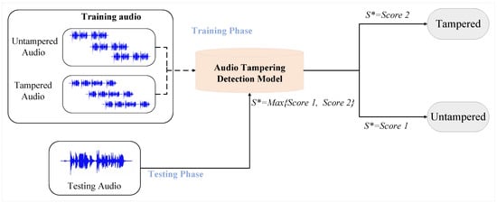
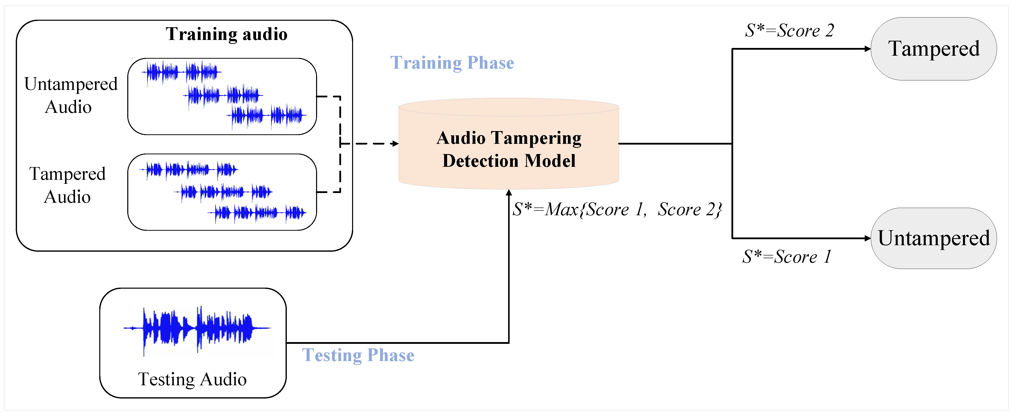
(Digital audio tampering detection task). The digital audio tampering detection task is divided into a training phase and a testing phase. In the training phase, our training audio is divided into tampered audio and untampered audio, after which these two classes of audio are trained to obtain the audio tampering detection model. In the testing phase, the test audio is fed into the audio tampering detection model to obtain two scores, i.e., the probability of belonging to the tampered and untampered categories. When , the audio belongs to the untampered audio class; when , the audio belongs to the tampered audio class. The flowchart of the digital audio tampering detection task is shown in Figure 1.

Figure 1.
Digital audio tampering detection task flowchart, where and denote the probabilities of tampered and untampered categories and denotes the maximum of and .
3.2. ENF Shallow Temporal and Spatial Feature Definition
Definition 2.
(ENF shallow temporal features). We frame the ENF phase based on the way the ENF temporal variation is performed to obtain the ENF shallow temporal feature , where is the number of phase points contained in a frame and is the number of frames.
Definition 3.
(ENF shallow spatial features). Since the ENF phase changes abruptly when audio tampering occurs, we design a framing method for the static features of the phase sequence to extract the shallow spatial features of the ENF, where m is the dimension of the shallow spatial features.
3.3. ENF Deep Temporal and Spatial Feature Definition
Definition 4.
(ENF deep temporal features). Deep temporal features are extracted from by RDTCN. Deep temporal features are extracted from ENF shallow temporal features using deep learning, which requires the use of networks with sequence modeling capabilities, such as Recurrent Neural Networks (RNN) and Long Short-Term Memory (LSTM). In this paper, we use a modified TCN to extract deep temporal features that reflect the temporal information in the feature data, including the analysis of similarity information and mutation information between neighboring frames, as well as the analysis of long-term fluctuation information.
Definition 5.
(ENF deep spatial features). Deep spatial features are extracted by CNN from . The deep spatial features of ENF extracted by the CNN have a larger perceptual field and richer information than the shallow features.
4. Methods
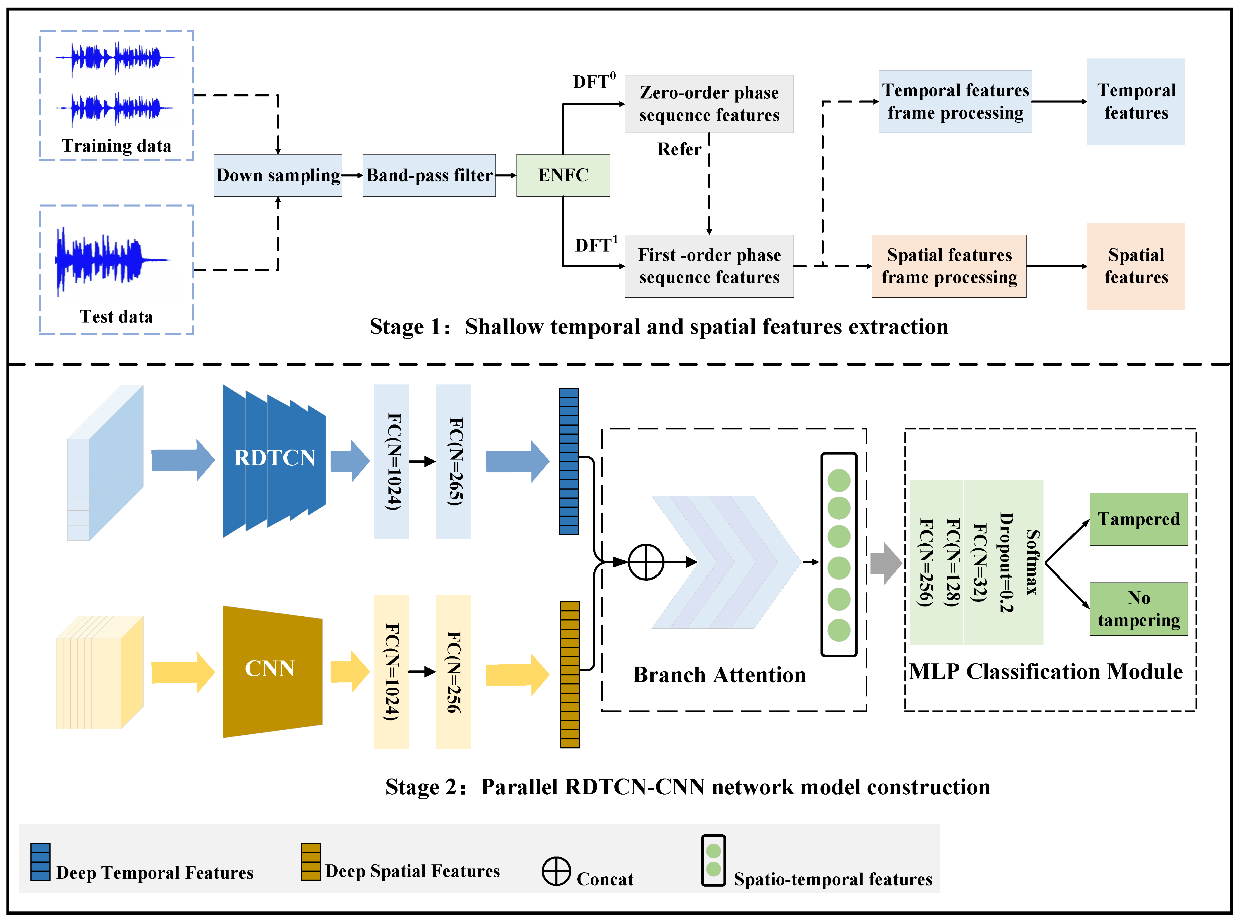
We propose a digital audio tampering detection method based on ENF deep temporal–spatial features. The method is mainly divided into two parts: ENF shallow temporal and spatial features extraction and the construction of a parallel RDTCN-CNN network model. In ENF shallow temporal and spatial feature extraction, firstly, the ENF first-order phase sequence feature is extracted based on [6]; then, it is divided into frames by adaptive frameshifting to obtain a phase feature matrix of the same size to represent the spatial features of ENF; at the same time, it is divided into frames according to the ENF phase temporal change information to represent the temporal features of the ENF. In the parallel RDTCN-CNN network model, we first extract deep temporal and spatial features using RDTCN and CNN, respectively, then use the branch attention mechanism to achieve deep temporal and spatial feature fusion, and finally complete the tampering detection by the MLP network. The framework of the digital audio tampering detection method based on ENF deep temporal–spatial feature is shown in Figure 2.
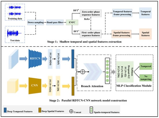
Figure 2.
A framework diagram of digital audio tampering detection based on ENF deep temporal–spatial feature, the model is divided into two steps: (1) shallow temporal and spatial feature extraction and (2) parallel RDTCN-CNN network model construction.
4.1. Extraction of the Shallow Temporal and Spatial Features of ENF
Because ENF has temporal and spatial information, we can extract it by different frame processing methods. The steps of extracting ENF shallow temporal and spatial features include: extracting ENF first-order phase sequence, extracting ENF shallow temporal features, and extracting ENF shallow spatial features.
4.1.1. Extraction of First-Order Phase Features
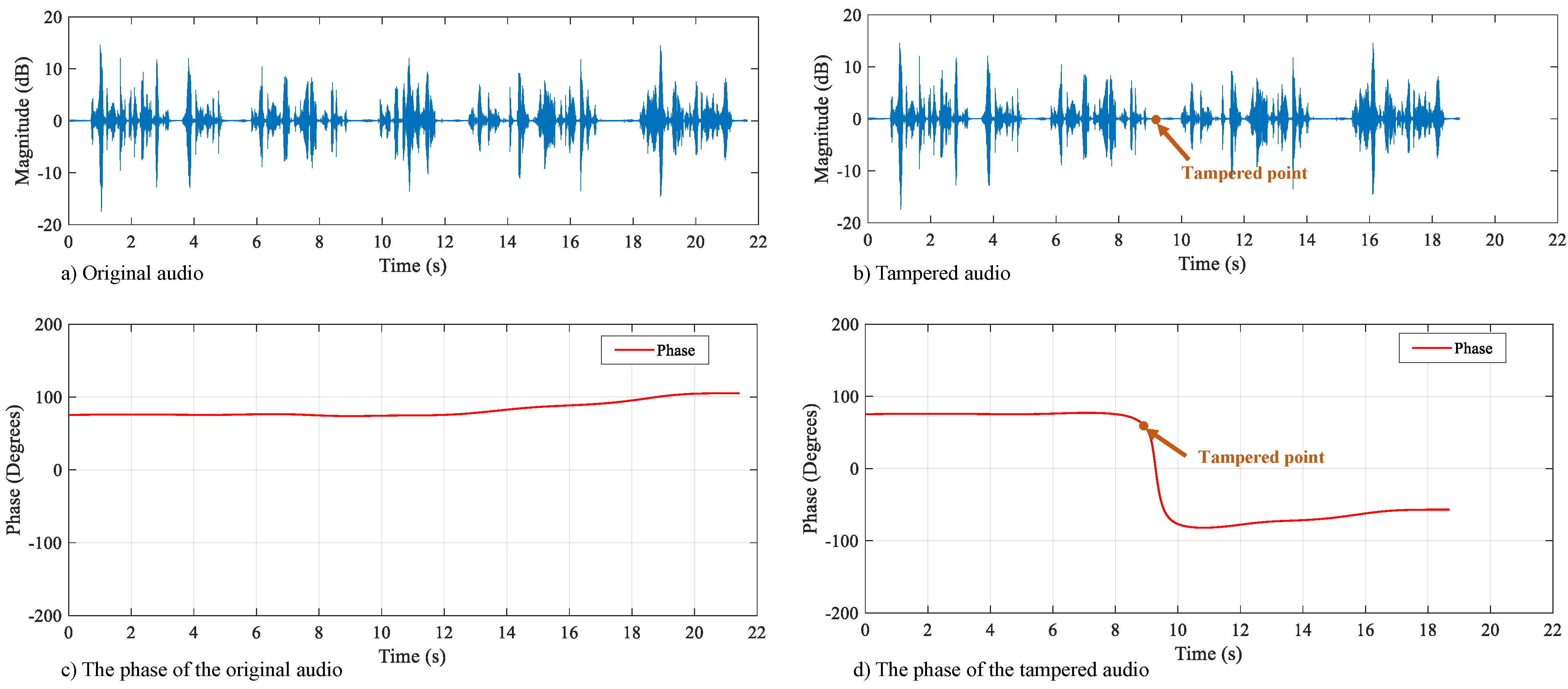
When the digital audio has been tampered with, the phase of the ENF changes abruptly at the tampered position, as shown in Figure 3. We achieve tampering detection of digital audio by representing the ENF phase features and performing consistency analysis on them.
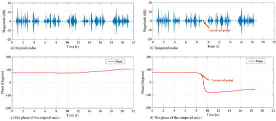
Figure 3.
Phase curve diagramof the original and tampered audio. (a) is the waveform graph of the original audio, (b) is the waveform graph of the tampered audio. When the audio is not tampered with, the phase curve is relatively smooth, as shown in (c). The phase of the audio; when phase tampering occurs, the phase curve changes abruptly at the point of tampering, as shown in (d). The phase of the tampered audio, where the audio undergoes a tampering operation of deletion at around 9 s.
To extract the first-order phase feature of the ENF, the ENFC in digital audio is first extracted by downsampling and band-pass filtering. Then, the ENFC is subjected to to estimate the ENF first-order phase sequence feature , where denotes the transform of the kth-order derivative of the signal [6].
To extract the ENFC from the digital audio, firstly, the digital audio signal to be measured is downsampled to obtain the downsampled signal , where the downsampling frequency is set to 1000 Hz or 1200 Hz. Secondly, we use bandpass filtering to narrowband filter the downsampled signal to obtain the ENFC in the signal to be measured.
To estimate the phase information more accurately, we use to further extract the first-order phase sequence information . First, we calculate the approximate first-order derivatives of the ENF signal at point n. The equation to obtain the first-order derivative signal is as follows:
Secondly, a window is added to the first-order derivative signal . Then, the transform is applied to and to obtain and , respectively. We estimate the frequency values based on as follows:
where and . is a scale function. Finally, we use the method to estimate , which is as follows:
where . There are two possible values of the solution of . In this paper, we use as a reference and choose the value of that is closest to as the final solution. We perform linear interpolation of to obtain the value of . is calculated as follows:
where , . represents the largest integer less than i, and represents the largest integer greater than j. , and is the downsampling frequency. The specific process is shown in Algorithm 1.
| Algorithm 1 Extraction of first-order phase features . |
|
4.1.2. Extraction of ENF Shallow Temporal Features
Various information and phase sequences of ENF change with its non-periodic fluctuations. In this paper, we propose a new framing algorithm based on the way of ENF timing variation to obtain the ENF shallow temporal feature , where is the number of phase points contained in a frame, which is an artificially set value. Since the setting of affects the amount of information contained in the ENF phase timing over a period of time, we will experiment with as a variable for the ENF temporal representation in the subsequent part of this paper. In addition, digital audio is often unequal in length, corresponding to its ENF first-order phase sequence. To reduce the loss of ENF temporal information, we calculate the number of frames from the longest audio. Based on the set frame length , the number of frames can be calculated as follows:
where is the maximum value of the ENF phase sequence. The frameshift is calculated as follows:
where the is rounded down. Finally, the shallow temporal feature is obtained by traversing the phase information of ENF by frameshift . The specific process is shown in Algorithm 2.
| Algorithm 2 Temporal feature frame processing of ENF. |
|
4.1.3. Extraction of ENF Shallow Spatial Features
When digital audio is tampered with, the ENF phase features cause abrupt changes [17]. To represent the static mutation information in the phase sequence, we designed a framing method for the static features of the phase sequence to extract the shallow spatial feature of the ENF. The extracted phase sequence features are of different lengths due to the unequal duration of each sample in the dataset. To reduce the information loss in the feature extraction process, we calculate the frame length m by the longest phase in the audio, which is as follows:
where , and is rounded upward. Then, the frameshift and subframe are calculated, and the frameshift is as follows:
The shallow spatial feature matrix is obtained by giving an adaptive frameshift of unequal audio phase sequences to facilitate automatic learning of the CNN. The specific process is shown in Algorithm 3.
| Algorithm 3 Spatial feature frame processing of ENF. |
|
4.2. Deep Feature Representation Learning Based on RDTCN-CNN Temporal–Spatial Feature Fusion
Based on and extracted in Section 4.1, we design a parallel RDTCN-CNN model to implement digital audio tampering passive detection, as shown in step 2 of Figure 2. The parallel RDTCN-CNN model is divided into three main stages: extraction of deep temporal and spatial features, the fusion of temporal and spatial features, and classification decision.
In the extraction stage of deep temporal and spatial features, we input the shallow temporal features into the RDTCN for representation learning to obtain the deep temporal features, while the shallow spatial features are input into the CNN for representation learning to obtain the deep spatial features. In the fusion stage of deep temporal and spatial features, we use the branch attention mechanism to fuse the deep temporal and spatial features of different branches to obtain the temporal–spatial features with stronger representation capability. In the classification decision stage, we input the temporal–spatial features to the MLP network to determine whether the audio has been tampered with.
4.2.1. Deep Temporal Feature Extraction Based on RDTCN Network
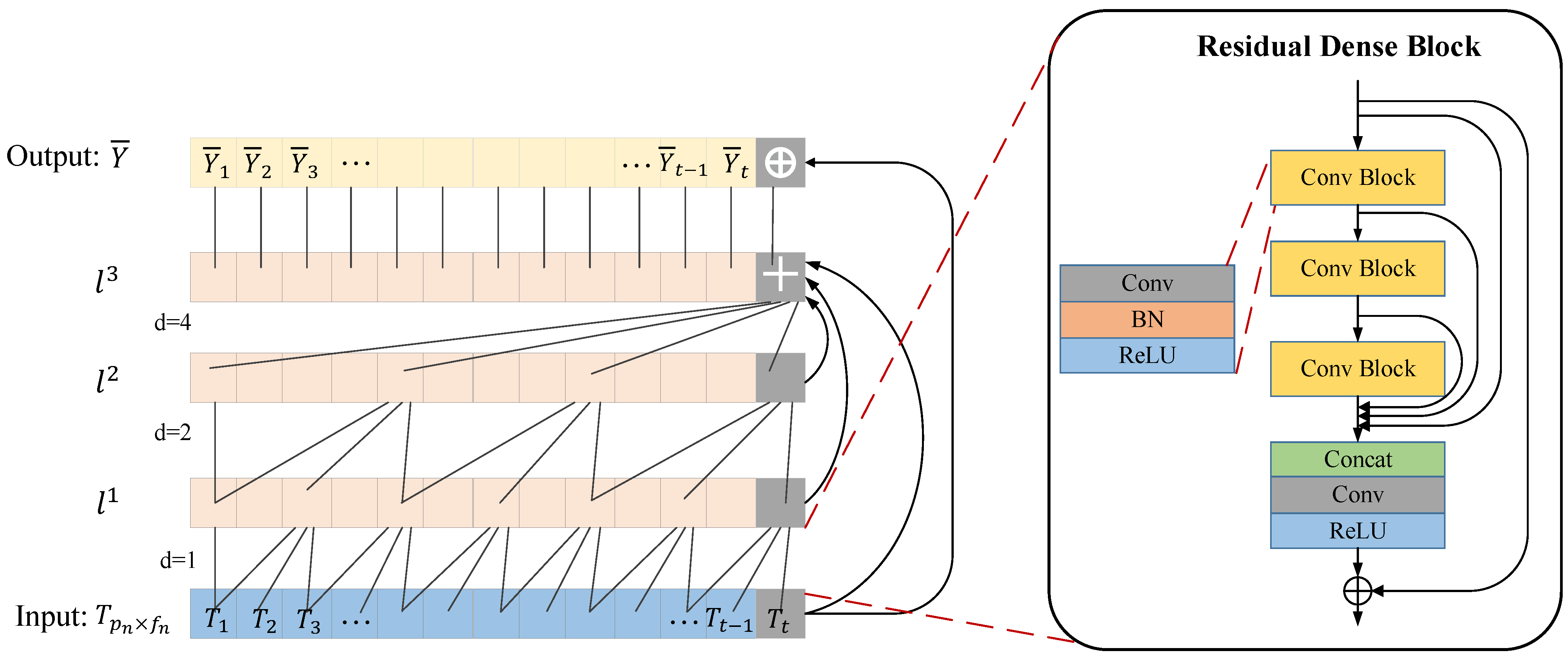
As the network deepens, the ordinary TCN network comes with residual layers and each convolutional layer has different layer-size perceptual fields. However, the deep temporal feature extraction network based on the ordinary TCN network neglects to make full use of the information of different receptive fields in each convolutional layer. This means that the common TCN network has a common residual structure, which causes the intermediate convolutional layers to not directly transfer information to the subsequent layers, so the memory block does not fully utilize the information of all the convolutional layers inside it. In order to improve the disadvantage of underutilized ordinary TCN memory blocks, we construct an RDTCN network using residual dense blocks and then extract the ENF deep temporal features. The RDTCN further improves information utilization compared with the ordinary TCN network. The RDTCN network structure is shown in Figure 4.

Figure 4.
RDTCN network structure figure (l: activation values in the l-th layer, d: dilation rate, +: concatenate operation, ⊕: add operation).
To address the shortcomings of ordinary residual networks, such as the inability to utilize feature information between each layer in the ENF deep temporal feature extraction task, a residual dense network is proposed instead of the ordinary residual blocks. The residual dense network is composed of a residual network and a dense network, with the residual network extracting global features and the dense convolutional layer extracting local features. In the dense connection, each layer of information fusion combines the inputs of all previous layers and uses cascading to propagate the features of the current layer to all subsequent layers, which is more effective in mitigating gradient disappearance and enhancing the propagation of all features, making the probability of feature reusability greater. The residual dense network combines the characteristics of the residual network and dense network to form a continuous memory mechanism by fusing global features and local features, which is implemented by linking the features extracted from the previous residual dense block to all layers of the current residual dense block. The residual dense block supports continuous memory, and after extracting multiple layers of local dense features, it will further fuse the global features and then retain the layered features in a global manner adaptively, thus producing implicit deep supervision.
The RDTCN mainly consists of causal convolution, dilated convolution, and residual dense modules. In causal convolution, a sequence is input, and a sequence is output after the operation of the model. The output at time t is only convolved with the historical elements before time t, thus ensuring that the future input will not affect the past input data prediction.
By adding holes to the standard convolution to expand the field of perception, the output data can contain a larger range of information without losing data in the pooling layer. The dilated convolution formula is as follows:
where the input sequence , filter , d is the expansion factor, c is the filter size, and denotes the past direction. The value of d relates to the size of the perceptual field, and d grows exponentially by 2.
In the residual dense block, each residual dense block is a combination of Conv -BN-ReLU, and the residual block is as follows:
where is the input of the lth residual dense block, is the output of the lth residual dense block, and denotes the last convolutional layer that performs the splicing operation on the output of the feature from all the convolutional layers in the brackets. The structure of the residual dense network is shown in the residual dense block in Figure 4, where means convolution, means batch normalization, means activation function, and the convolution kernel size is with a step size of 1.
4.2.2. Deep Spatial Feature Extraction Based on CNN Network
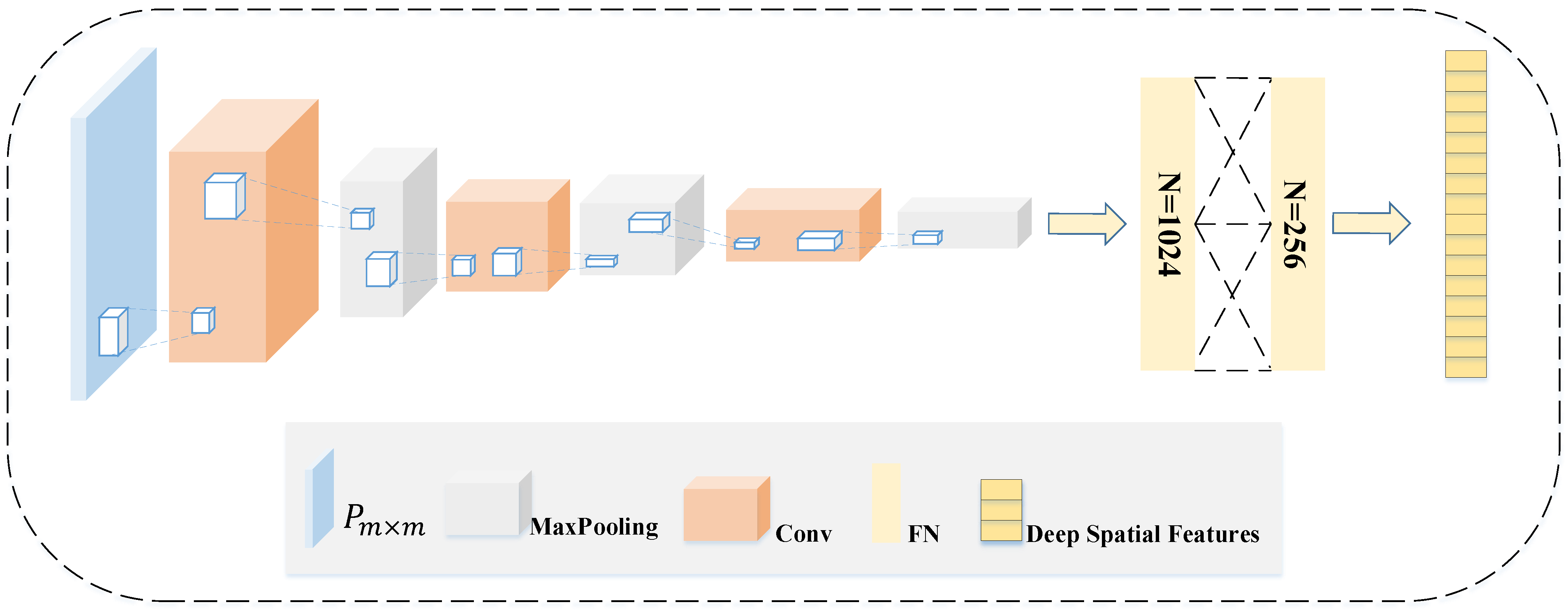
In this section, in order to extract the deep spatial features of ENF quickly and efficiently, we design a CNN to implement the extraction of deep spatial features, as shown in Figure 5.

Figure 5.
Based on the CNN deep space feature extraction module, the network input is the shallow space features , m is 45, and the output is the deep space features extracted by the CNN network.
CNN is a multilayer feedforward neural network that has been shown to have outstanding performance in extracting spatial features. The sparse connectivity and weight-sharing nature of the CNN greatly reduce the number of model parameters. The sparse connectivity and weight-sharing nature of the CNN allow it to learn audio features with less computational effort, with stable results, and without additional feature engineering requirements on the data.
The CNN consists of a convolutional layer and a pooling layer. The convolutional layer further extracts the deep spatial features by convolving the input shallow spatial features. The input to the deep space feature extraction module of CNN is , which has dimensions (45, 45). The deep spatial feature extraction module consists of three convolutional layers, three pooling layers, and two fully connected layers. The number of convolutional kernels is 16, 32, 64, and the size of the kernels is (3, 3). convolutional kernels can increase the number of network layers compared to larger convolutional kernels, which also increases the nonlinear expression capability of the network and reduces the network parameters. After each convolutional layer, a MaxPooling layer of size (2, 2) is set. The high-level feature map obtained after pooling not only reduces the dimensionality and number of parameters of the original feature map, but also avoids problems such as overfitting. After the convolutional pooling of multiple layers, the Flatten layer is connected to transform the multidimensional data into one-dimensional data to realize the transition from the convolutional layer to the fully connected layer. The number of nodes in the first fully connected layer is 1024, and the number of nodes in the second fully connected layer is 256. The convolutional layer cooperates with the pooling layer to extract local features of spatial features, then connects with the fully connected layer to extract the global features and finally obtains deep spatial features.
4.2.3. Deep Temporal and Spatial Feature Fusion Based on Branch Attention Mechanism
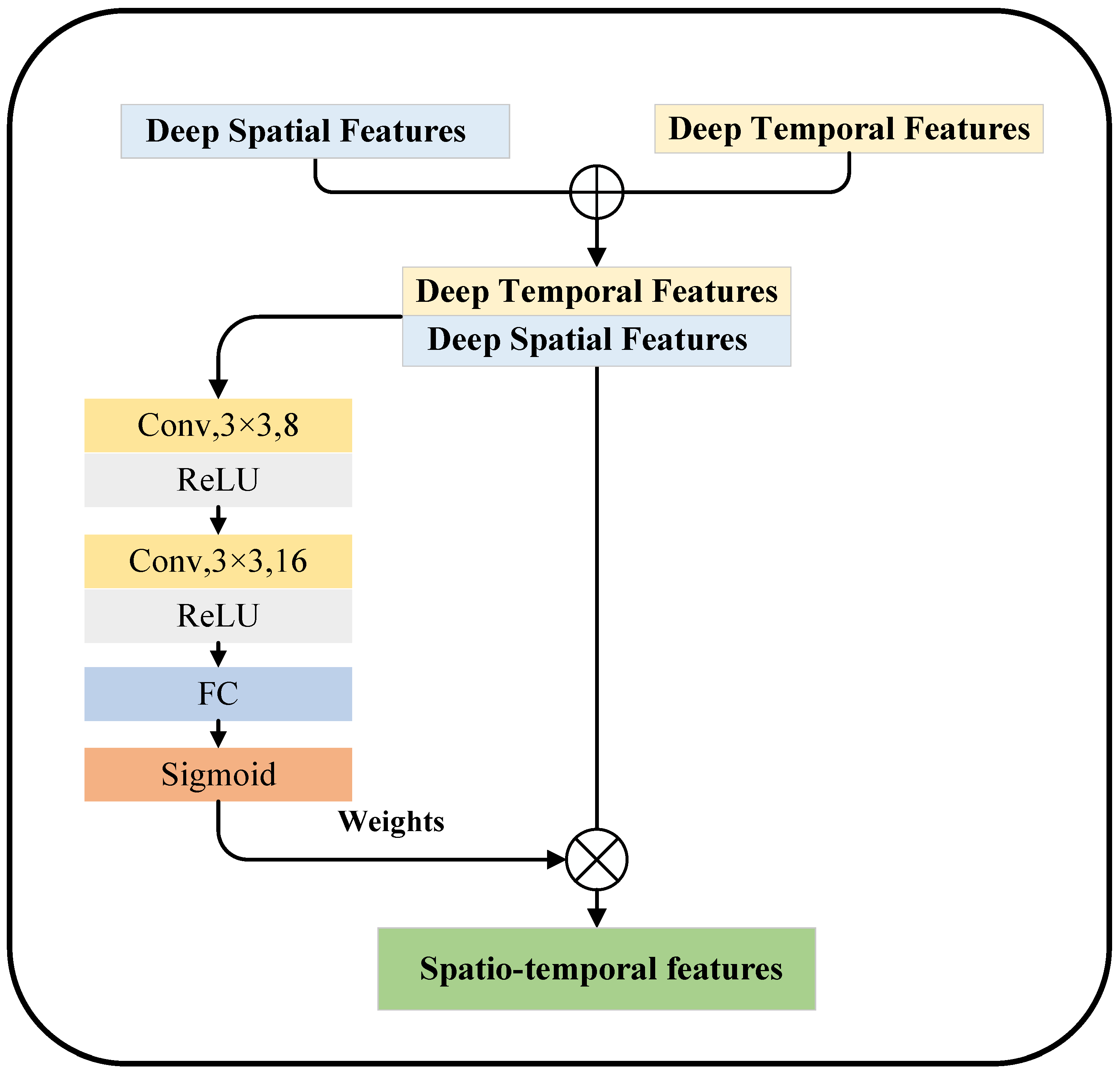
Because deep temporal and spatial features are extracted from different branches of the parallel RDTCN-CNN, we choose the branch attention mechanism for deep temporal and spatial feature fusion to achieve the fusion of temporal and spatial features. The branch attention mechanism can achieve linear fusion of deep temporal features with deep spatial features when performing the feature fusion task. The equation of the branch attention mechanism is as follows:
where and are, respectively, the deep temporal and spatial features, is the join operation, is the spliced feature and is the convolutional pooling operation in the branch attention mechanism, and reflects the deep temporal–spatial features after fusion.
In addition, this mechanism assigns weights to different types of features through network learning, so that important features have more prominent representational power in model training. The branch attention fusion mechanism includes weight learning and dot product assignment. In weight learning, we learn useful information in deep temporal and spatial features by convolutional operations. In the dot product assignment, we dot product the learned weights with the spliced deep temporal–spatial and spatial features to adaptively assign the weights and obtain the temporal–spatial features with stronger representational ability, as shown in Figure 6.

Figure 6.
Branch attention mechanism, where ⊕ is the operation and ⊗ is the dot product.
4.2.4. Classification Network Design
In this section, we use the MLP classification network to determine whether it has been tampered with. The network consists of four fully connected layers (the number of neurons is 256, 128, 32, and the activation function is ), a Dropout layer (dropout rate = 0.2), and a layer, and the specific network structure is shown in Figure 2. layer can output the binary classification results for determining whether the audio has been tampered with or not, and the formula is as follows:
where is the predicted value of the output, numbers the output features of the previous layer, W is the weight, and b is the bias.
Our loss function adopts binary cross entropy. This is a commonly used loss function in binary classification problems, and its expression is as follows:
where N is the number of audio data, y corresponds to the label value of each voice, and is the probability that the output belongs to label y. is the value of the binary cross entropy loss function, which is used to judge the performance of our model.
5. Experimental Results and Analysis
To validate the effectiveness of the proposed method, we conducted a large number of experiments on different audio datasets. To validate the effectiveness of each independent part of the framework, we followed the idea of the controlled variable method to conduct an ablation study to observe the core modules and key hyperparameters of our method.
5.1. Dataset
In this paper, Carioca [25,47], New Spanish [52], and ENF_Audio are used as experimental data. The detailed statistics of these datasets are shown in Table 2.

Table 2.
Dataset information.
Carioca consists of Carioca 1 [25] and Carioca 2 [47], a database of speech signals from telephone recordings on the public switched telephone network (PSTN), both with an ENF of 60 Hz. Cariocacontains 500 speech signals. The audio in Carioca 1 was all sampled at 44.1 kHz, with a word length of 16 bits, a bit rate of 705 kbps, a single channel, a file format of WAV, and a signal-to-noise ratio (SNR) ranging from 16 dB to 30 dB (22.3 dB on average). Carioca 1 has a total of 200 audio signals, and the audio signals range from 19 to 35 s in duration. There were 100 of these original audio signals, including 50 male and 50 female. For each gender, 25 signals were copied and 25 signals were cut, resulting in another 100 tampered audios, where each signal was copied or cut only once. Carioca 2 had a sampling frequency of 11,050 Hz, a word length of 16, a bit rate of 176 kbps, a single channel, a file format of WAV, and a signal-to-noise ratio of 10.1 dB to 30 dB (the average Carioca 2 file contains a total of 300 signals with durations of 9 to 25 seconds). There were 150 raw audios, including 75 male and 75 female. An additional 150 tampered signals were obtained by performing a delete or insert operation on all 150 original audios. The processing was carried out in the same way as in Carioca 1.
New Spanish [52] comes from two public Spanish databases, AHUMADA and GAUDI, containing stable 50 Hz ENFCs, which also contain 753 speech signals. All signals have a sampling rate of 8 kHz, a word length of 16, a bit rate of 128 kbps, a single channel, a file format of WAV, and an average signal-to-noise ratio of 35 dB. There were 251 original audio files. The 502 tampered audio files were obtained by deletion and insertion operations.
ENF_Audio is our database, consisting of a random mix of Carioca and New Spanish, with a total of 1253 audio signals.
5.2. Evaluation Metrics
Tampering detection of digital audio is a complex task involving multiple domains of security. To verify the reliability of the model, we cite feedback prediction as the main evaluation task. In the experiments of this paper, we use prediction accuracy (ACC) and F1-score (F1-score) as evaluation metrics.
is the error between the prediction result and the actual feedback, demonstrating the most significant value and progress of the model. The higher the Accuracy, the higher the precision. The formula for prediction accuracy is:
where is predicted to be positive and actually positive, is predicted to be negative and actually negative, is predicted to be positive and actually negative, and is predicted to be negative and actually positive. The ACC is calculated using the evaluate function in the Keras library. (The API address for Evaluate is at https://keras.io/api/models/model_training_apis/ (accessed on 10 April 2023))
is the result of combining the output of Precision (P) and Recall (R), and the ranges from 0 to 1, with 1 representing the best output of the model and 0 representing the worst output of the model. The formula for the is as follows:
where P represents the precision rate, which is given by the formula: , and R represents the recall rate, which is given by the formula: . The F1-score is calculated using the metrics function in the Scikit-learn library. (The API address for Metrics is at https://scikit-learn.org/stable/modules/generated/sklearn.metrics.f1_score.html (accessed on 10 April 2023))
5.3. Baselines
To evaluate the performance of our model, we need other baselines for comparison. The details of the baselines are as follows: [25] and [26] are two classical tamper detection methods. Therefore, we use them as baselines. In addition, in our previous work, [6] is a new method proposed based on the advantages of the above two methods [25,26], so we also use it as a baseline. [5] is a new audio tampering detection method from the perspective of temporal feature representation learning, so we also use it as a baseline.
[25] estimated the phase of ENFC by discrete Fourier variation and used SVM for classification.
[26] used ESPRIT to estimate the characteristics of the phase peak and used SVM for classification.
[6] used , , and Hilbert transform to extract the phase and instantaneous frequency of ENFC and used an optimized SVM for the classification of tamper detection.
[5] divides the extracted phase features into frames, and each frame is represented as the information of ENF phase change over a period of time, and then the BI-LSTM network is used to obtain the difference information between real audio and tampered audio, and finally, a DNN classifier is used for classification.
5.4. Experimental Settings
Hardware Setting: In this paper, experiments were conducted on a professional computer with an NVIDIA TITAN RTX high-performance graphics card. The CPU is an I7-9700, the GPU is an RTX TITAN X, and the running memory is 64 GB.
Software Setting: Audio framing, windowing, filtering, and parameter extraction were performed on MATLAB R2020a. Our model simulations were performed on Python 3.6, Tensorflow 1.15, Keras 2.1.5, Numpy 1.19, Pandas 0.25, etc.
Framework Setting: The shallow spatial feature has an m of 46, the shallow temporal feature has a of 85 and of 25, the loss function is Binary_Crossentropy, the optimizer is Adam, the training epoch is 300, the batch size is 64, and the initial learning rate is 0.001. The training set, validation set, and test set are divided into 7:1:2.
5.5. Results and Discussion
To verify the effectiveness of the method in this paper, we demonstrate the effectiveness of the features and classification models in this section and the superiority of the method through four sets of experiments. The experiments are designed as follows: (1) comparison with baseline methods; (2) verifying the effectiveness of RDTCN temporal feature extraction network; (3) verifying the effect of frame length setting on the shallow temporal features of ENF; (4) verifying the effectiveness of the branch attention mechanism.
5.5.1. Comparison with Baseline Methods
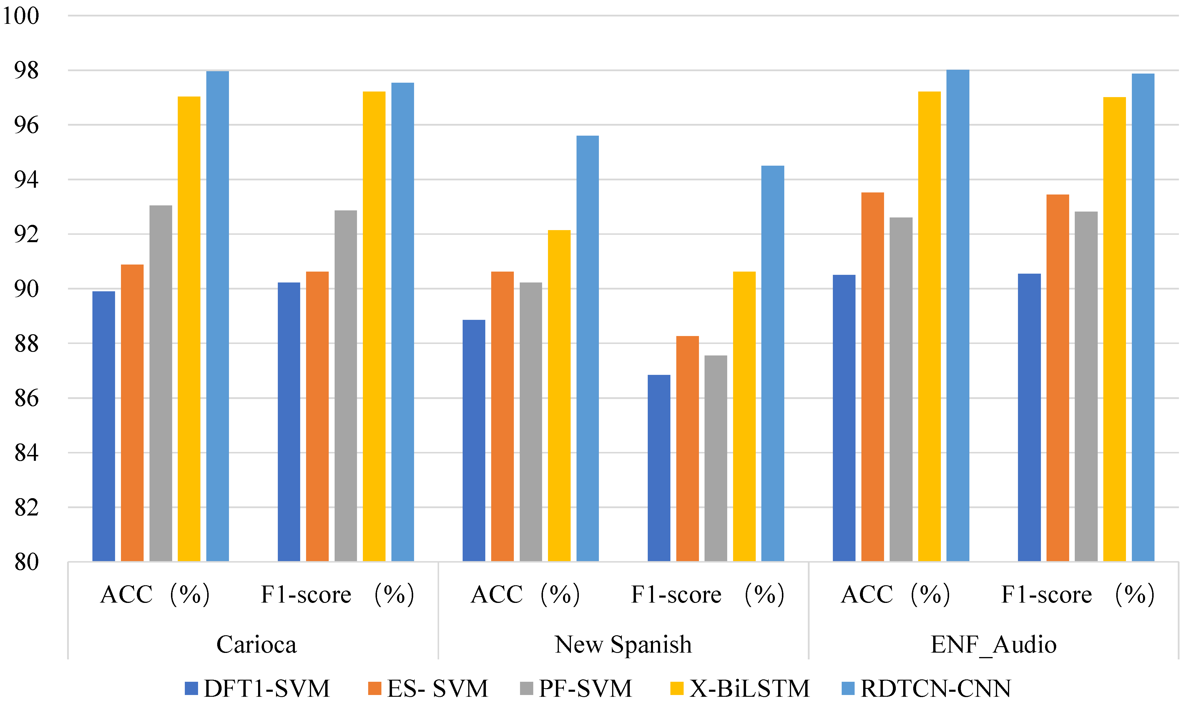
In order to verify the effectiveness of our proposed digital audio tampering detection method, we compare the proposed method RDTCN-CNN with the method of baseline [5,6,25,26] in the public Carioca, New Spanish, and ENF_Audio datasets, and the experimental results are shown in Table 3.

Table 3.
Comparison with baseline.
From the results, it can be seen that the and of X-BiLSTM and the method in this paper are much higher than the other three methods for the same dataset [6,25,26]. Both X-BiLSTM [5] and RDTCN-CNN use deep-learning methods, which have better performance in extracting key information in features compared to classical machine learning. For both methods using deep learning, the method in this paper uses a parallel RDTCN-CNN network to extract both spatial and temporal information of ENF. In comparison, the X-BiLSTM only utilizes temporal information in the ENF phase and ignores information on ENF phase space, and is 1.20% higher than X-BiLSTM in terms of accuracy.
As can be seen in Figure 7, the and of RDTCN-CNN in different datasets are higher than the other four baseline methods, which verifies the effectiveness of this method.
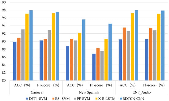
Figure 7.
Comparison between this method and the four baseline methods under different datasets and different evaluation indexes, respectively. DFT1-SVM, ES-SVM, PF-SVM, and X-BiLSTM are the baseline methods, RDTCN-CNN is this paper’s method, and are the evaluation metrics, and Carioca, New Spanish, and ENF_Audio are the three audio tampering detection databases.
5.5.2. Verifying the Effectiveness of the RDTCN Temporal Feature Extraction Network
To verify the effectiveness of RDTCN networks, a set of comparison experiments based on ordinary TCN temporal feature extraction and RDTCN temporal feature based on shallow spatial feature extraction networks are conducted in this section, both of which adopt the structure of CNN.
In the RDTCN temporal feature extraction network, the original residual blocks of the TCN network are replaced with residual dense blocks. From the experimental results in Table 4, it can be seen that the ordinary TCN temporal feature extraction network based on the RDTCN achieves 97.42%, while the TCN network with the addition of residual dense blocks achieves 98.02%, which is an accuracy improvement of 0.6% to 98.02% compared to the ordinary TCN temporal feature extraction network. In addition, the RDTCN temporal feature extraction network also improves the by 0.42% compared to the normal TCN temporal feature extraction network. Different evaluation metrics are sufficient to prove that the RDTCN temporal feature extraction network is effective and that the features in the layered convolution in the TCN network are effective for the digital audio tampering detection task.

Table 4.
Comparison of RDTCN and ordinary TCN.
5.5.3. Verifying the Effect of Frame Length Setting on the Shallow Temporal Features of ENF
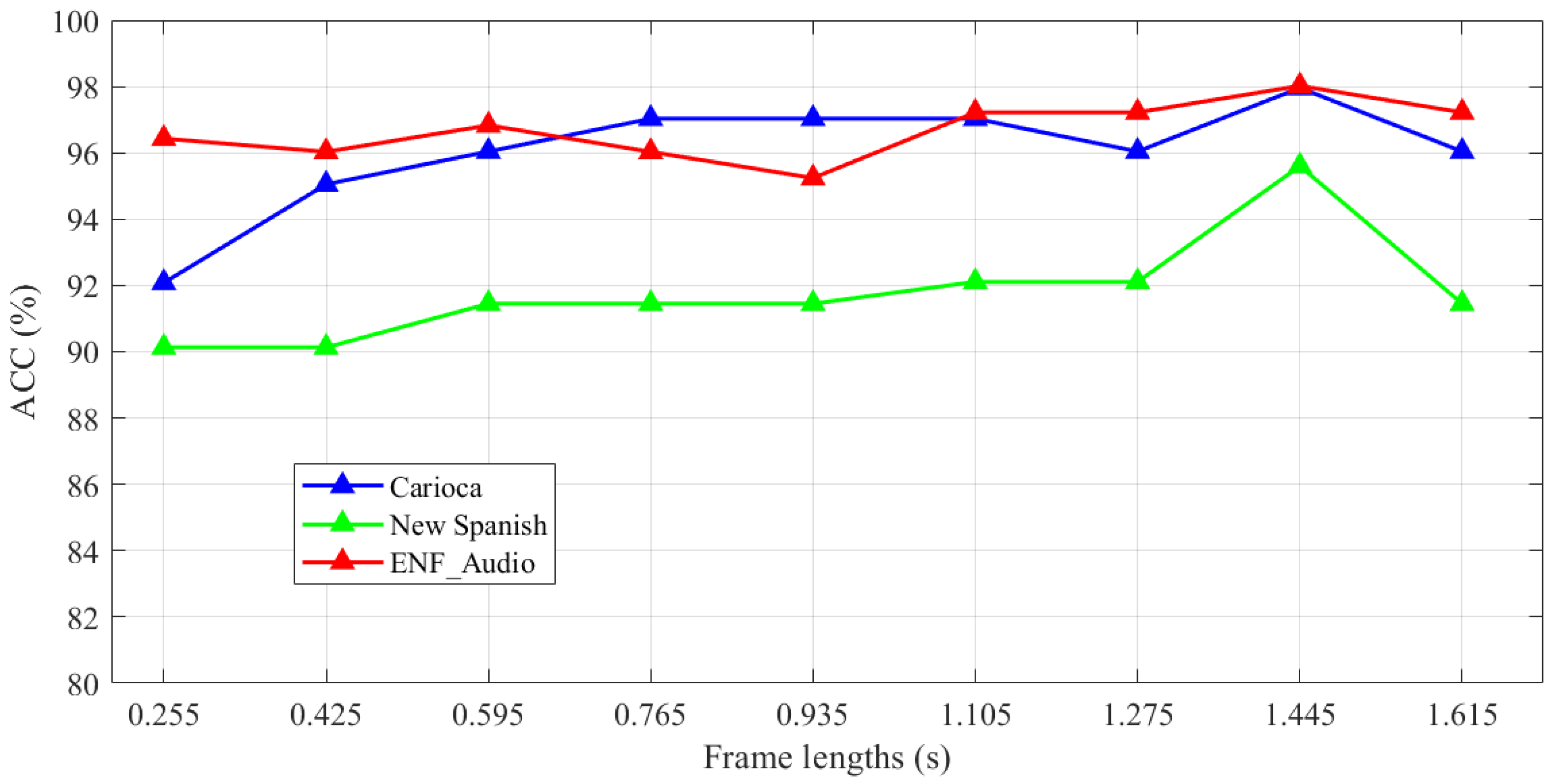
The digital audio signal is a time-varying signal, and various information of audio and parameters characterizing its basic features change with time but remain basically unchanged in a short period of time, so the audio signal has long-term fluctuation and short-term stability. Every 0.17 s contains 10 phase points, and the phase number determines the amount of information of ENF phase change in a short time. A suitable frame length setting can better represent the fluctuation of temporal information and is more conducive to the extraction of temporal information by the RDTCN network. In order to analyze the effect of frame length on features, we conducted comparison experiments on the frame length settings of ENF shallow temporal features on Carioca, New Spanish, and ENF_Audio datasets, and nine experimental groups were set in the frame length range of 0.255 s∼1.615 s, and the accuracy variation curves with frame length are shown in Figure 8.
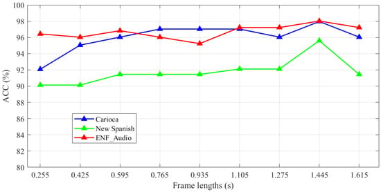
Figure 8.
Comparison between this method and the four baseline methods under different datasets and different evaluation indexes, respectively.
From the experimental results, we can see that the detection accuracy is high when the frame length is 0.595 s and the number of phase points per unit frame is 35, the accuracy tends to decrease after the frame length is 1.445 s, and the number of phase points per unit frame is 85. Since the highest accuracy is achieved when the frame length is 1.445 s and the number of phase points per unit frame is 85, we choose the frame length of 1.445 s, the number of phase points per unit frame of 85, and the number of frames of 25 as the parameters of the ENF shallow temporal feature .
5.5.4. Verifying the Effectiveness of the Branch Attention Mechanism
To verify the effect of branch attention mechanism on parallel RDTCN-CNN, we designed a comparison experiment between the feature fusion network based on the splicing structure and the feature fusion network based on the branch attention mechanism. The former uses the splicing layer to replace the attention mechanism module to achieve the fusion of deep temporal and spatial features, and the other network parameters remain unchanged.
The experimental results are shown in Table 5. With our parallel RDTCN-CNN network, based on the attention mechanism, the Carioca, New Spanish, and ENF_Audio datasets all show significant improvement in accuracy compared to the parallel RDTCN -CNN network based on the splicing structure. This proves that the branch attention mechanism is effective for different types of feature weight distributions. Through adaptive learning, the attention mechanism can give more weight to the features that are useful for classification and suppress the invalid features, thus improving detection accuracy.

Table 5.
A comparative experiment of branch attention mechanisms.
6. Conclusions
In this paper, we propose a digital audio tampering detection method based on ENF deep temporal–spatial features. Structurally, our method includes the extraction of shallow temporal and spatial features of ENF and the construction of parallel RDTCN-CNN network models. For the extraction of shallow temporal and spatial features, the phase sequence of ENF is first extracted by using the high-precision discrete Fourier analysis method. Secondly, for the information on different dimensions of ENF, shallow temporal and spatial features are extracted using different frame processing methods. In the construction of a parallel RDTCN-CNN network model, we use RDTCN, which is good at processing temporal signals, to further extract deep temporal features, and use CNN network, which is good at extracting spatial features, to further extract deep spatial features, and realize the fusion of temporal–spatial features by the branch attention mechanism. Finally, the MLP network is used to determine whether the digital audio has been tampered with or not. The experimental results show that our proposed method has a high accuracy and F1-score in the Carioca, New Spanish, and ENF_Audio databases, outperforming the four baseline methods.
The method in this paper represents only the phase features of the ENF, while the harmonic signal, spectrogram, and many other features of the ENF should be equally valued. Moreover, the research in this paper focuses on whether the audio has been tampered with and only addresses the basic issues. Further analysis is still needed to determine the deeper location of tampering and the specific type of tampering. Therefore, in future work, deeper mining of more features in the ENF and further analysis of tampering locations and tampering types are necessary. In addition, we need to further automate the filtering and feature extraction of the original audio waveform through the network model and implement end-to-end tasks in the model to make it applicable to more complex scenarios to facilitate applications.
Author Contributions
Conceptualization, Z.W. and C.Z.; methodology, Z.W. and C.Z.; software, S.K.; validation, Z.W., K.L., Y.Z. and C.Z.; formal analysis, Z.W. and C.Z.; investigation, Z.W. and C.Z.; resources, Z.W. and C.Z.; data curation, Z.W. and C.Z.; writing—original draft preparation, Z.W. and C.Z.; writing—review and editing, Z.W. and C.Z.; visualization, Z.W., K.L., Y.Z. and C.Z.; supervision, Z.W.; project administration, Z.W.; funding acquisition, Z.W. and C.Z. All authors have read and agreed to the published version of the manuscript.
Funding
The research work in this paper was supported by the National Natural Science Foundation of China (No. 62177022, 61901165), AI and Faculty Empowerment Pilot Project (No. CCNUAI&FE2022-03-01), Collaborative Innovation Center for Informatization and Balanced Development of K-12 Education by MOE and Hubei Province (No. xtzd2021-005), National Natural Science Foundation of China (No. 61501199), and Natural Science Foundation of Hubei Province (No. 2022CFA007).
Informed Consent Statement
This study did not involve humans.
Data Availability Statement
Data will be made available on reasonable request.
Conflicts of Interest
The authors declare no conflict of interest.
Abbreviations
The following abbreviations are used in this manuscript:
| ENF | Electrical Network Frequency |
| RDTCN | Residual Dense Temporal Convolutional Networks |
| CNN | Convolutional Neural Networks |
| MLP | Multilayer Perceptron |
| MFCC | Mel Frequency Cepstral Coefficient |
| SVM | Support Vector Machine |
| ENFC | ENF Component |
| RFA | Robust Filtering Algorithm |
| PSTN | Public Switched Telephone Network |
| RNN | Recurrent Neural Networks |
| LSTM | Long Short-Term Memory |
References
- Liu, Z.; Lu, W. Fast Copy-Move Detection of Digital Audio. In Proceedings of the 2017 IEEE Second International Conference on Data Science in Cyberspace (DSC), Shenzhen, China, 26–29 June 2017; pp. 625–629. [Google Scholar] [CrossRef]
- Zeng, C.; Zhu, D.; Wang, Z.; Wang, Z.; Zhao, N.; He, L. An End-to-End Deep Source Recording Device Identification System for Web Media Forensics. Int. J. Web Inf. Syst. 2020, 16, 413–425. [Google Scholar] [CrossRef]
- Yan, Q.; Yang, R.; Huang, J. Detection of Speech Smoothing on Very Short Clip. IEEE Trans. Inf. Forensics Secur. 2019, 9, 2441–2453. [Google Scholar] [CrossRef]
- Wang, Z.; Yang, Y.; Zeng, C.; Kong, S.; Feng, S.; Zhao, N. Shallow and Deep Feature Fusion for Digital Audio Tampering Detection. EURASIP J. Adv. Signal Process. 2022, 2022, 1–20. [Google Scholar] [CrossRef]
- Zeng, C.; Yang, Y.; Wang, Z.; Kong, S.; Feng, S. Audio Tampering Forensics Based on Representation Learning of ENF Phase Sequence. Int. J. Digit. Crime Forensics 2022, 14, 1–19. [Google Scholar] [CrossRef]
- Wang, Z.F.; Wang, J.; Zeng, C.Y.; Min, Q.S.; Tian, Y.; Zuo, M.Z. Digital Audio Tampering Detection Based on ENF Consistency. In Proceedings of the 2018 International Conference on Wavelet Analysis and Pattern Recognition (ICWAPR) IEEE, Chengdu, China, 15–18 July 2018; pp. 209–214. [Google Scholar] [CrossRef]
- Hua, G.; Liao, H.; Wang, Q. Detection of Electric Network Frequency in Audio Recordings–From Theory to Practical Detectors; IEEE Press: Piscataway, NJ, USA, 2021; Volume 1, pp. 1556–6013. [Google Scholar] [CrossRef]
- Hajj-Ahmad, A.; Garg, R.; Wu, M. Instantaneous frequency estimation and localization for ENF signals. In Proceedings of the 2012 Asia Pacific Signal and Information Processing Association Annual Summit and Conference IEEE, Hollywood, CA, USA, 3–6 December 2012; pp. 1–10. [Google Scholar]
- Bykhovsky, D. Recording Device Identification by ENF Harmonics Power Analysis. Forensic Sci. Int. 2020, 307, 110100. [Google Scholar] [CrossRef] [PubMed]
- Zeng, C.; Zhu, D.; Wang, Z.; Wu, M.; Xiong, W.; Zhao, N. Spatial and Temporal Learning Representation for End-to-End Recording Device Identification. EURASIP J. Adv. Signal Process. 2021, 2021, 41. [Google Scholar] [CrossRef]
- Lin, X.; Zhu, J.; Chen, D. Subband Aware CNN for Cell-Phone Recognition. IEEE Signal Process. Lett. 2020, 27, 5. [Google Scholar] [CrossRef]
- Verma, V.; Khanna, N. Speaker-Independent Source Cell-Phone Identification for Re-Compressed and Noisy Audio Recordings. Multimed. Tools Appl. 2021, 80, 23581–23603. [Google Scholar] [CrossRef]
- Meng, X.; Li, C.; Tian, L. Detecting Audio Splicing Forgery Algorithm Based on Local Noise Level Estimation. In Proceedings of the 2018 5th International Conference on Systems and Informatics (ICSAI), Nanjing, China, 10–12 November 2018; pp. 861–865. [Google Scholar] [CrossRef]
- Lin, X.; Kang, X. Exposing speech tampering via spectral phase analysis. Digit. Signal Process. 2017, 1, 63–74. [Google Scholar] [CrossRef]
- Yan, D.; Dong, M.; Gao, J. Exposing Speech Transsplicing Forgery with Noise Level Inconsistency. Secur. Commun. Netw. 2021, 1, 6. [Google Scholar] [CrossRef]
- Narkhede, M.; Patole, R. Acoustic scene identification for audio authentication. Soft Comput. Signal Process. 2021, 1, 593–602. [Google Scholar]
- Capoferri, D.; Borrelli, C. Speech Audio Splicing Detection and Localization Exploiting Reverberation Cues. In Proceedings of the 2020 IEEE International Workshop on Information Forensics and Security (WIFS), New York, NY, USA, 6–11 December 2020; pp. 1–6. [Google Scholar] [CrossRef]
- Jadhav, S.; Patole, R.; Rege, P. Audio Splicing Detection using Convolutional Neural Network. In Proceedings of the 2019 10th International Conference on Computing, Communication and Networking Technologies (ICCCNT), Kanpur, India, 6–8 July 2019; pp. 1–5. [Google Scholar] [CrossRef]
- Saleem, S.; Dilawari, A.; Khan, U. Spoofed Voice Detection using Dense Features of STFT and MDCT Spectrograms. In Proceedings of the 2021 International Conference on Artificial Intelligence (ICAI), Islamabad, Pakistan, 5–7 April 2021; pp. 56–61. [Google Scholar] [CrossRef]
- Li, C.; Sun, Y.; Meng, X. Homologous Audio Copy-move Tampering Detection Method Based on Pitch. In Proceedings of the 2019 IEEE 19th International Conference on Communication Technology (ICCT), Xi’an, China, 16–19 October 2019; pp. 530–534. [Google Scholar] [CrossRef]
- Yan, Q.; Yang, R.; Huang, J. Robust Copy–Move Detection of Speech Recording Using Similarities of Pitch and Formant. IEEE Trans. Inf. Forensics Secur. 2019, 9, 2331–2341. [Google Scholar] [CrossRef]
- Xie, X.; Lu, W.; Liu, X. Copy-move detection of digital audio based on multi-feature decision. J. Inf. Secur. Appl. 2018, 10, 37–46. [Google Scholar] [CrossRef]
- Lin, X.; Kang, X. Supervised audio tampering detection using an autoregressive model. In Proceedings of the 2017 IEEE International Conference on Acoustics, Speech and Signal Processing (ICASSP), New Orleans, LA, USA, 5–9 March 2017; pp. 2142–2146. [Google Scholar] [CrossRef]
- Hua, G.; Liao, H.; Zhang, H. Robust ENF Estimation Based on Harmonic Enhancement and Maximum Weight Clique. IEEE Trans. Inf. Forensics Secur. 2021, 7, 3874–3887. [Google Scholar] [CrossRef]
- Nicolalde, D.; Apolinario, J. Audio Authenticity: Detecting ENF Discontinuity With High Precision Phase Analysis. IEEE Trans. Inf. Forensics Secur. 2010, 9, 534–543. [Google Scholar] [CrossRef]
- Reis, P.; Lustosa, J.; Miranda, R. ESPRIT-Hilbert-Based Audio Tampering Detection With SVM Classifier for Forensic Analysis via Electrical Network Frequency. IEEE Trans. Inf. Forensics Secur. 2017, 4, 853–864. [Google Scholar] [CrossRef]
- Zakariah, M.; Khan, M.; Malik, H. Digital multimedia audio forensics: Past, present and future. Multimed. Tools Appl. 2017, 1, 1009–1040. [Google Scholar] [CrossRef]
- Bai, Z.; Zhang, X.L. Speaker Recognition Based on Deep Learning: An Overview. Neural Netw. 2021, 140, 65–99. [Google Scholar] [CrossRef]
- Mohd Hanifa, R.; Isa, K.; Mohamad, S. A Review on Speaker Recognition: Technology and Challenges. Comput. Electr. Eng. 2021, 90, 107005. [Google Scholar] [CrossRef]
- Wang, Z.; Wang, Z.; Zeng, C.; Yu, Y.; Wan, X. High-Quality Image Compressed Sensing and Reconstruction with Multi-Scale Dilated Convolutional Neural Network. Circuits Syst. Signal Process. 2022, 42, 1–24. [Google Scholar] [CrossRef]
- Abdu, S.A.; Yousef, A.H.; Salem, A. Multimodal Video Sentiment Analysis Using Deep Learning Approaches, a Survey. Inf. Fusion 2021, 76, 204–226. [Google Scholar] [CrossRef]
- Bayoudh, K.; Knani, R.; Hamdaoui, F.; Mtibaa, A. A Survey on Deep Multimodal Learning for Computer Vision: Advances, Trends, Applications, and Datasets. Vis. Comput. 2022, 38, 2939–2970. [Google Scholar] [CrossRef]
- Chango, W.; Lara, J.A.; Cerezo, R.; Romero, C. A Review on Data Fusion in Multimodal Learning Analytics and Educational Data Mining. WIREs Data Min. Knowl. Discov. 2022, 12, e1458. [Google Scholar] [CrossRef]
- Dimitri, G.M. A Short Survey on Deep Learning for Multimodal Integration: Applications, Future Perspectives and Challenges. Computers 2022, 11, 163. [Google Scholar] [CrossRef]
- Gandhi, A.; Adhvaryu, K.; Poria, S.; Cambria, E.; Hussain, A. Multimodal Sentiment Analysis: A Systematic Review of History, Datasets, Multimodal Fusion Methods, Applications, Challenges and Future Directions. Inf. Fusion 2023, 91, 424–444. [Google Scholar] [CrossRef]
- Han, X.; Wang, Y.T.; Feng, J.L.; Deng, C.; Chen, Z.H.; Huang, Y.A.; Su, H.; Hu, L.; Hu, P.W. A Survey of Transformer-Based Multimodal Pre-Trained Modals. Neurocomputing 2023, 515, 89–106. [Google Scholar] [CrossRef]
- He, K.; Zhang, X.; Ren, S.; Sun, J. Deep Residual Learning for Image Recognition. In Proceedings of the IEEE Conference on Computer Vision and Pattern Recognition, Las Vegas, NV, USA, 27–30 June 2016; pp. 770–778. [Google Scholar]
- Krizhevsky, A.; Sutskever, I.; Hinton, G.E. ImageNet Classification with Deep Convolutional Neural Networks. In Proceedings of the Advances in Neural Information Processing Systems, Lake Tahoe, NV, USA, 3–6 December 2012; Volume 25. [Google Scholar]
- Wang, Z.; Yan, W.; Zeng, C.; Tian, Y.; Dong, S. A Unified Interpretable Intelligent Learning Diagnosis Framework for Learning Performance Prediction in Intelligent Tutoring Systems. Int. J. Intell. Syst. 2023, 2023, 1–20. [Google Scholar] [CrossRef]
- Wu, T.; Ling, Q. Self-Supervised Heterogeneous Hypergraph Network for Knowledge Tracing. Inf. Sci. 2023, 624, 200–216. [Google Scholar] [CrossRef]
- Pan, X.; Zhang, X. Detecting splicing in digital audios using local noise level estimation. In Proceedings of the 2012 IEEE International Conference on Acoustics, Speech and Signal Processing (ICASSP), Kyoto, Japan, 25–30 March 2012; pp. 1841–1844. [Google Scholar] [CrossRef]
- Malik, H. Acoustic environment identification and its applications to audio forensics. IEEE Trans. Inf. Forensics Secur. 2013, 8, 1827–1837. [Google Scholar] [CrossRef]
- Mascia, M.; Canclini, A.; Antonacci, F. Forensic and anti-forensic analysis of indoor/outdoor classifiers based on acoustic clues. In Proceedings of the 2015 23rd European Signal Processing Conference (EUSIPCO), Nice, France, 31 August–4 September 2015; pp. 2072–2076. [Google Scholar] [CrossRef]
- Ikram, S.; Malik, H. Digital audio forensics using background noise. In Proceedings of the 2010 IEEE International Conference on Multimedia and Expo, Singapore, 19–23 July 2010; pp. 106–110. [Google Scholar] [CrossRef]
- Chen, J.; Xiang, S.; Huang, H. Detecting and locating digital audio forgeries based on singularity analysis with wavelet packet. Multimed. Tools Appl. 2016, 2, 2303–2325. [Google Scholar] [CrossRef]
- Imran, M.; Xiang, S.; Huang, H. Blind detection of copy-move forgery in digital audio forensics. IEEE Access 2017, 6, 12843–12855. [Google Scholar] [CrossRef]
- Esquef, P.A.A.; Apolinário, J.A.; Biscainho, L.W.P. Edit Detection in Speech Recordings via Instantaneous Electric Network Frequency Variations. IEEE Trans. Inf. Forensics Secur. 2014, 10, 2314–2326. [Google Scholar] [CrossRef]
- Mao, M.; Xiao, Z.; Kang, X.; Li, X. Electric Network Frequency Based Audio Forensics Using Convolutional Neural Networks. IFIP Adv. Inf. Commun. Technol. 2020, 8, 253–270. [Google Scholar] [CrossRef]
- Sarkar, M.; Chowdhury, D.; Shahnaz, C.; Fattah, S.A. Application of Electrical Network Frequency of Digital Recordings for Location-Stamp Verification. Appl. Sci. 2019, 9, 3135. [Google Scholar] [CrossRef]
- Karantaidis, G.; Kotropoulos, C. Blackman–Tukey spectral estimation and electric network frequency matching from power mains and speech recordings. IET Signal Process. 2021, 6, 396–409. [Google Scholar] [CrossRef]
- Hua, G.; Zhang, H. ENF Signal Enhancement in Audio Recordings. IEEE Trans. Inf. Forensics Secur. 2020, 11, 1868–1878. [Google Scholar] [CrossRef]
- Ortega-Garcia, J.; Gonzalez-Rodriguez, J. Audio Speech variability in automatic speaker recognition systems for commercial and forensic purposes. IEEE Aerosp. Electron. Syst. Mag. 2000, 11, 27–32. [Google Scholar] [CrossRef]
Disclaimer/Publisher’s Note: The statements, opinions and data contained in all publications are solely those of the individual author(s) and contributor(s) and not of MDPI and/or the editor(s). MDPI and/or the editor(s) disclaim responsibility for any injury to people or property resulting from any ideas, methods, instructions or products referred to in the content. |
© 2023 by the authors. Licensee MDPI, Basel, Switzerland. This article is an open access article distributed under the terms and conditions of the Creative Commons Attribution (CC BY) license (https://creativecommons.org/licenses/by/4.0/).

