On the Soundness of XAI in Prognostics and Health Management (PHM)

Abstract

The aim of predictive maintenance, within the field of prognostics and health management (PHM), is to identify and anticipate potential issues in the equipment before these become serious. The main challenge to be addressed is to assess the amount of time a piece of equipment will function effectively before it fails, which is known as remaining useful life (RUL). Deep learning (DL) models, such as Deep Convolutional Neural Networks (DCNN) and Long Short-Term Memory (LSTM) networks, have been widely adopted to address the task, with great success. However, it is well known that these kinds of black box models are opaque decision systems, and it may be hard to explain their outputs to stakeholders (experts in the industrial equipment). Due to the large number of parameters that determine the behavior of these complex models, understanding the reasoning behind the predictions is challenging. This paper presents a critical and comparative revision on a number of explainable AI (XAI) methods applied on time series regression models for PM. The aim is to explore XAI methods within time series regression, which have been less studied than those for time series classification. This study addresses three distinct RUL problems using three different datasets, each with its own unique context: gearbox, fast-charging batteries, and turbofan engine. Five XAI methods were reviewed and compared based on a set of nine metrics that quantify desirable properties for any XAI method. One of the metrics introduced in this study is a novel metric. The results show that Grad-CAM is the most robust method, and that the best layer is not the bottom one, as is commonly seen within the context of image processing.

1. Introduction

Incipient AI systems, as small decision trees, were interpretable but had limited capabilities. Nevertheless, during the last few years, the notable increase in the performance of predictive models (for both classification and regression) has been accompanied by an increase in model complexity. This has been at the expense of losing the understanding capacity of the reasons behind each particular prediction. This kind of model is known as a black-box [1] due to the opaqueness of its behavior. Such obscurity becomes a problem, especially when the predictions of a model impact different dimensions within the human realm (such as medicine, law, profiling, autonomous driving, or defense, among others) [2]. It is also important to note that opaque models are difficult to debug, as opposed to the interpretable ones, which facilitate the detection of the source of its errors/bias and the implementation of a solution [3].

1.1. Explainable Artificial Intelligence

Explainable AI (XAI) addresses these issues by proposing machine learning (ML) techniques that generate explanations of black-box models or create more transparent models (in particular for post hoc explainability) [4]. Post hoc explainability techniques can be divided into model-agnostic and model-specific techniques. Model-agnostic techniques encompass those that can be applied to any ML model, such as LIME [5] or SHAP [6] (SHapley Additive exPlanations), for example. Whereas model-specific techniques are designed for certain ML models, such as Grad-CAM (Gradient-weighted Class Activation Mapping) [7], saliency maps [8], or layer-wise relevance propagation (LRP) [9], which are focused on deep learning (DL) models.

Regarding the kind of tasks where XAI can be applied, it is common to find applications in classification tasks with tabular and image data, while regression tasks—signal processing, among others—have received little attention. The higher number of studies devoted to XAI for classification tasks is due to the ease of its application, since implicit knowledge exists around each class [10]. Similarly, there is not much work on XAI applied to time series models [11]. The non-intuitive nature of time series [12] makes them harder to be understood.

Several studies have applied XAI methods to regression time series. For instance, Ahmed et al. [13] used SHAP and LIME to explain the predictions of a model trained to forecast travel time. In another study, Vijayan [14] employed a deep learning multi-output regression model to predict the relationship between optical design parameters of an asymmetric Twin Elliptical Core Photonic Crystal Fiber (TEC-PCF) and its sensing performances. Then, they used SHAP for feature selection and to understand the effect of each feature on the model’s prediction. Mamalakis et al. [15] trained a fully connected neural network (NN) using a large ensemble of historical and future climate simulations to predict the ensemble- and global-mean temperature. They then applied various XAI methods and different baselines to attribute the network predictions to the input. Cohen et al. [16] proposed a new clustering framework that uses Shapley values and is compatible with semi-supervised learning problems. This framework relaxes the strict supervision requirement of current XAI techniques. Brusa et al. [17] examined the performance of the SHapley Additive exPlanation (SHAP) method in detecting and classifying faults in rotating machinery using condition monitoring data. Kratzert et al. [18] used integrated gradients to explain the predictions of a Long Short-Term Memory (LSTM) model trained for rainfall-runoff forecasting. Finally, Zhang et al. [19] presented a framework to explain video activity with natural language using a zero-shot learning approach through a Contrastive Language-Image Pre-training (CLIP) [20] model. This is a very interesting idea that could be useful to apply to time-series data to explain predictions in natural language.

In the same way that there does not exist a model best suited to solve any ML task, there is no particular XAI method that will provide the best explanation of any model. A significant body of literature devoted to innovations in novel interpretable models and explanation strategies can be found. However, quantifying the correctness of their explanations remains challenging. Most ML interpretability research efforts are not aimed at comparing the explanation quality (measuring it) provided by XAI methods [21,22]. It can find two types of indicators for the assessment and comparison of explanations: qualitative and quantitative. Quantitative indicators, which are the focus of this paper, are designed to measure desirable characteristics that any XAI method should have. The metrics approximate the level of accomplishment of each characteristic, thus allowing us to measure them on any XAI method. As these metrics are a form of estimating the accomplishment level, they will be referred to as proxies. Numerical proxies are useful to assess the explanation quality, providing a straightforward way to compare different explanations.

A (non-exhaustive) list of work on proxies shows its usefulness. In [11], Schlegel, et al. apply several XAI methods, usually used with models built from image and text data, and propose a methodology to evaluate them on time series. Samek, at al. [23] apply a perturbation method on the variables that are important in the prediction generation, to measure the quality of the explanation. The work of Doshi-Velez, et al. and Honegger [24,25] propose three proxies (called axioms in those works) to measure the consistency of explanation methods. The three proxies are identity (identical samples must have identical explanations), separability (non-identical samples cannot have identical explanations) and stability (similar samples must have similar explanations). There exists other work that proposes different proxies for more specific models or tasks [26].

1.2. XAI and Predictive Maintenance

The industrial maintenance process consists of three main stages. The first stage involves identifying and characterizing any faults that have occurred in the system. In the second stage, known as the diagnosis phase, the internal location of the defects is determined, including which parts of the system are affected and what may have caused the faults. In the final stage, known as the prognosis phase, the gathered information is used to predict the machine’s operating state, or remaining useful life (RUL) at any given time, based on a description of each system part and its condition. The first two are classification problems, while prognosis is commonly addressed as a regression problem. In the field of predictive maintenance (Pdm), there is an important lack of XAI methods for industrial prognosis problems [22] and it is difficult to find existing work in which new XAI methods are developed, or existing ones that are applied within this context. Hong, et al. [27] use SHAP to explain predictions in RUL prediction. Similarly, Szelazek, et al. [28] use an adaptation of SHAP for decision trees applied to steel production systems prognosis, to predict when the thickness of the steel is out of specifications. Serranilla, et al. [29] apply LIME to models used in the estimation of bushings remaining time of life. Recently, Ferrano, et al. [30] have applied SHAP and LIME in hard disk drive failure prognosis.

1.3. Aim and Structure of the Paper

Raw signal time series are frequently voluminous, and it is challenging to analyze the data. Due to this issue, a quantitative method must verify the quality of explanations [11]. This paper considers five XAI methods to address regression tasks on signal time series; specifically, for system prognosis within the context of prognostics and health management (PHM). Two of them, SHAP and LIME, are model-agnostic XAI methods. The other three (layer-wise relevance propagation, gradient activation mapping, and saliency maps) are neural network specific. It is worth noting that all these methods have been adapted in this paper to work with time series regression models.

This article aims to present several contributions to the field of Explainable Artificial Intelligence. Firstly, it presents a comprehensive review of eight existing proxy methods for evaluating the interpretability of machine learning models. Secondly, it proposes a novel proxy to measure the time-dependence of XAI methods, which has not been previously explored in the literature. Thirdly, an alternative version of Grad-CAM is proposed, which takes into account both the time and time series dimensions of the input, improving its interpretability. Finally, the importance of layers in Grad-CAM for explainability is evaluated using the proposed proxies.

The article is organized into five main sections. Section 2 covers the Materials and Methods used in the study, including the XAI methods and the perturbation and neighborhood techniques. Section 2.3 focuses on the validation of the XAI method explanations using quantitative proxies. Section 3 provides details on the experiments conducted in the study, including the datasets (Section 3.2) and the black-box models used (Section 3.3). Section 3.4 describes the experiments themselves, and Section 3.5 presents the results of the study. Finally, Section 4 provides a discussion of the findings and their implications.

2. Materials and Methods

This section describes the different XAI methods under investigation (Section 2.1), as well as the consistency of explanation proxies used in the experiments carried out (Section 2.2).

2.1. XAI Methods

This section provides a brief description of the XAI models used in the experiments.

2.1.1. Local Interpretable Model-Agnostic Explanations

Local interpretable model-agnostic explanations (LIME) [5] is an XAI method based on a surrogate model. In XAI, surrogate models are trained to approximate the predictions of the black-box model. These models would be white-box models, easily interpreted (sparse linear models or simple decision trees). In the case of LIME, the surrogate model is trained to approximate an individual prediction and the predictions of its neighborhood obtained by perturbing the individual sample studied. The LIME surrogate model is trained with a data representation of the original sample $xϵR^d$. The representation uses $x^{\prime }ϵ{\{0,1\}}^{d^{\prime }}$ to state the non-perturbation/perturbation of each original feature. Mathematically, the explanations obtained with LIME can be expressed as:

$$\xi \left(x\right)=\underset{gϵG}{argmin}\mathcal{L}(f,g,{\pi }_x)+\mathsf{\Omega }\left(g\right)$$

(1)

where g is a surrogate model from the class G of the all interpretable models. The component $\mathsf{\Omega }\left(g\right)$ is used as regularization to keep the complexity of g low, since high complexity is opposed to the interpretability concept. The model being explained is denoted as f and $\mathcal{L}$ determines the performance of g fitting the locality defined by $\pi$ as a proximity measurement function and ${\pi }_x=\pi (x,·)$. Finally, each training sample is weighted with the distance between the perturbed sample and the original sample.

2.1.2. SHapley Additive exPlanations

SHapley Additive exPlanations (SHAP) [6] is also a method to explain individual predictions, similarly to LIME. The SHAP method explains each feature by computing Shapley values from coalitional game theory. A Shapley value can be described as the expected average of a player’s marginal contribution (by considering all possible combinations). It enables the determination of a payoff for all players, even when each one has contributed differently. In SHAP, each feature is considered a player. Thus, the coalition vector $x^{\prime }$, or simplified features vector, is composed of ones and zeroes representing the presence or absence of a feature, respectively. The contribution of each feature ${\varphi }_i$ is estimated based on its marginal contribution [31], and computed as follows:

$${\varphi }_i(f,x)=\sum _{z^{\prime }\subseteq x^{\prime }}\frac{\left|z^{\prime }\right|!(M-\left|z^{\prime }\right|-1)!}{M!}\left[f_x\left(z^{\prime }\right)-f_x(z^{\prime }\setminus i\right)]$$

(2)

where $\left|z^{\prime }\right|$ is the number of non-zero entries in $z^{\prime }$, and $z^{\prime }\subseteq x^{\prime }$ represents all vectors where the non-zero entries are a subset of the coalition vector $x^{\prime }$. The values ${\varphi }_i$ are known as Shapley values, and it has been demonstrated that they satisfy the properties of local accuracy, missingness, and consistency [6]. Based on these contribution values, a linear model is defined to obtain the explainable model g:

$$g\left(x^{\prime }\right)={\varphi }_o+\underset{j=1}{\sum ^M}{\varphi }_j$$

(3)

The explainable model g is optimized by minimizing the mean squared error between g and the predictions over the perturbed samples $f\left(h_x\left(z^{\prime }\right)\right)$. The main difference to LIME is that, in SHAP, each sample is weighted based on the number of ones in $z^{\prime }$. The weighting function, called the weighting kernel, gives rise to the so-called Kernel SHAP method. The formula for the weight ${\pi }_x\left(z^{\prime }\right)$ is given by:

$${\pi }_x\left(z^{\prime }\right)=\frac{(M-1)}{\left(\genfrac{}{}{0pt}{}{M}{\left|z^{\prime }\right|}\right)(M-\left|z^{\prime }\right|)}$$

(4)

The intuition behind this is that isolating features provides more information about their contribution to the prediction. This approach computes only the more informative coalitions, as computing all possible combinations is an intractable problem in most cases.

2.1.3. Layer-Wise Relevance Propagation

The Layer-wise Relevance Propagation (LRP) method [9] aims to interpret the predictions of deep neural networks. It is thus a model-specific XAI method. The goal is to attribute relevance scores to each input feature (or neuron) of a neural network, indicating its contribution to the final prediction. LRP works by propagating relevance scores from the output layer of the network back to its input layer. The relevance scores are initialized at the output layer: a score of 1 is assigned to the neuron corresponding to the predicted class and 0 to all others. Then, relevance is propagated backward from layer to layer using a propagation rule that distributes the relevance scores among the inputs of each neuron in proportion to their contribution to the neuron’s output. The rule ensures that the sum of relevance scores at each layer is conserved. The propagation rule is defined by the equation.

$$R_i=\sum _k\frac{z_{ik}}{{\sum }_{0,j}{z}_{jk}}{R}_k$$

(5)

where R represents the propagation relevance score, j and k refer to neurons in two consecutive layers, and $z_{jk}=a_j{w}_{jk}$ denotes how neuron j influences the relevance of neuron k based on the activation of each neuron. The denominator enforces the conservation property.

2.1.4. Image-Specific Class Saliency

Image-Specific Class Saliency [8] is one of the earliest pixel attribution methods existing in the literature. Pixel attribution methods aim to explain the contribution of each individual pixel, within an image, to the model’s output. These methods are typically used in computer vision tasks such as image classification or object detection. However, in this paper, attribution is assigned to each element of each time series, rather than individual pixels in an image. It is based on approximating the scoring or loss function, $S_c\left(x\right)$, with a linear relationship in the neighborhood of x:

$$S_c\left(x\right)\approx w_c^{T}x+b$$

(6)

where each element of $w_c$ is the importance of the corresponding element in x. The $w_c$ vector of importance values is computed via the derivative of $S_c$ with respect to the input x:

$$w=\frac{\partial S_c}{\partial x}{|}_{x_0}$$

(7)

This method was originally designed to work in Image Processing with neural networks, hence each element of w is associated with the importance of each pixel.

2.1.5. Gradient-Weighted Class Activation Mapping

Finally, Gradient-weighted Class Activation Mapping (Grad-CAM) generalizes CAM [32], which determines the significance of each neuron in the prediction by considering the gradient information that flows into the last convolutional layer of the CNN. Grad-CAM computes the gradient $y^c$ of class c with respect to a feature map $A^k$ of a convolutional layer, which is then globally averaged, obtaining the neural importance ${\alpha }_k^c$ of the feature map $A^k$:

$${\alpha }_k^c=\stackrel{globalaveragepooling}{\overbrace{\frac{1}{Z}\sum _i\sum _j}}\underset{gradientsviabackprop}{\underbrace{\frac{\partial y^c}{\partial A^k}}}$$

(8)

After computing the importance of all feature maps, a heat map can be obtained through a weighted combination of them. The authors apply a ReLU activation since they are only interested in positive importance;

$$L^c=ReLU\left(\sum _k{\alpha }_k^c{A}^k\right)$$

(9)

Unlike saliency maps, Grad-CAM associates importance by regions of the input. The size of them depends on the size of the convolutional layer. Usually, interpolation is applied to the original heat map to expand it to the overall size of the input.

As this paper is focused on time series, we propose introducing additional elements to Grad-CAM with the aim of exploiting the possible stationary information of the signal. This is achieved by introducing an additional component to the Grad-CAM heat map calculation, namely the time component contribution. Moreover, a second component was introduced to exploit the importance each time series has in a multivariate time series problem. Thus, the final Grad-CAM attribution equation reads as follows, namely, the individual time series contribution:

$${\alpha }_k^c=\stackrel{individualfeaturecontribution}{\overbrace{\frac{1}{T\ast F}\stackrel{T}{\sum _i}\stackrel{F}{\sum _j}\frac{\partial y^c}{\partial A^k}}}+\underset{timecomponentcontribution}{\beta \underbrace{\frac{1}{T}\stackrel{T}{\sum _i}\frac{\partial y^c}{\partial A^k}}}+\stackrel{individualtimeseriescontribution}{\overbrace{\sigma \frac{1}{F}\stackrel{F}{\sum _j}\frac{\partial y^c}{\partial A^k}}}$$

(10)

where T and F are the time units present in the time series, and the number of time series, respectively. The components $\beta$ and $\sigma$ are used to weight these two new components.

Figure 1 displays examples of heat maps generated by each method. Each heat map is a matrix of 20 by 160 values, representing 20 time series and 160 time units, where a relative importance is assigned to each item in the time series.

2.2. Perturbation and Neighborhood

The LRP, saliency map, and Grad-CAM techniques can be used directly on time series data. However, LIME and SHAP assume that significant changes in the performance of a well-trained model will occur if its relevant features (time points) are altered. Due to the high dimensionality of time series inputs, in order to achieve the former, it is necessary to specify a grouping of time series elements to analyze the impact on each group instead of on single time points. In image processing, this is achieved through super-pixels, which are groups of connected pixels that share a common characteristic.

In this paper, time series are segmented considering adjacent elements. Two different segmentation approaches are used. The first one is called uniform segmentation, which is the most basic method, and involves splitting the time series $ts=t_0,t_1,t_2,\dots ,t_n$ into equally sized windows without overlapping. The total number of windows is $d=\frac{n}{m}$, where m is the size of the window. If n is not divisible by m, the last window may be adjusted. The second segmentation minimizes the sum of $l2$ errors by grouping time points as follows:

$${ϵ}_{l2}\left(t{s}_{i,j}\right)=\stackrel{j}{\sum _{k=i}}{\left|t{s}_k-{\overline{ts}}_{i,j}\right|}^2$$

(11)

where $t{s}_{i,j}$ represents a segment of the time series signal $ts$ that goes from element i to element j, and $\overline{t{s}_{i,j}}$ is the mean of that segment. That is to say, the final cost of the segmentation is the sum of the $l2$ errors, calculated between each pair of adjacent elements within the segment. To find the optimal segmentation, a dynamic programming approach is employed, similarly to that described in [33]. The two segmentation strategies are shown in Figure 2.

Once the segmentation is complete, a perturbation method must be applied to create the neighborhood of the time series for SHAP and LIME. The following five perturbation techniques have been applied on the segmented time series in the different experiments carried out:

• Zero: The values in $t{s}_{i,j}$ are set to zero.
• One: The values in $t{s}_{i,j}$ are set to one.
• Mean: The values in $t{s}_{i,j}$ are replaced with the mean of that segment (${\overline{ts}}_{i,j}$).
• Uniform Noise: The values in $t{s}_{i,j}$ are replaced with random noise following a uniform distribution between the minimum and maximum values of the feature.
• Normal Noise: The values in $t{s}_{i,j}$ are replaced with random noise following a normal distribution with mean and standard deviation of the feature.

To obtain a perturbed sample $x^{\prime }$, firstly, it is divided into n segments. Then, from this segmentation, a binary representation $z^{\prime }$, identifying which segments will be perturbed, is randomly generated:

$$x^{\prime }=h(x,z^{\prime })=\left(h{(x,z^{\prime })}_1,h{(x,z^{\prime })}_2,...,h{(x,z^{\prime })}_n\right)$$

(12)

where

$$h{(x,z^{\prime })}_i=\left\{\begin{array}{cc}g(x,i)& if{z}_i^{\prime }isequal0\\ p\left(g\right(x,i\left)\right)& if{z}_i^{\prime }isequal1\end{array}\right.i\in \{1,...,n\}$$

(13)

with p being a perturbation function and g a segmentation function.

2.3. Validation of XAI Method Explanations

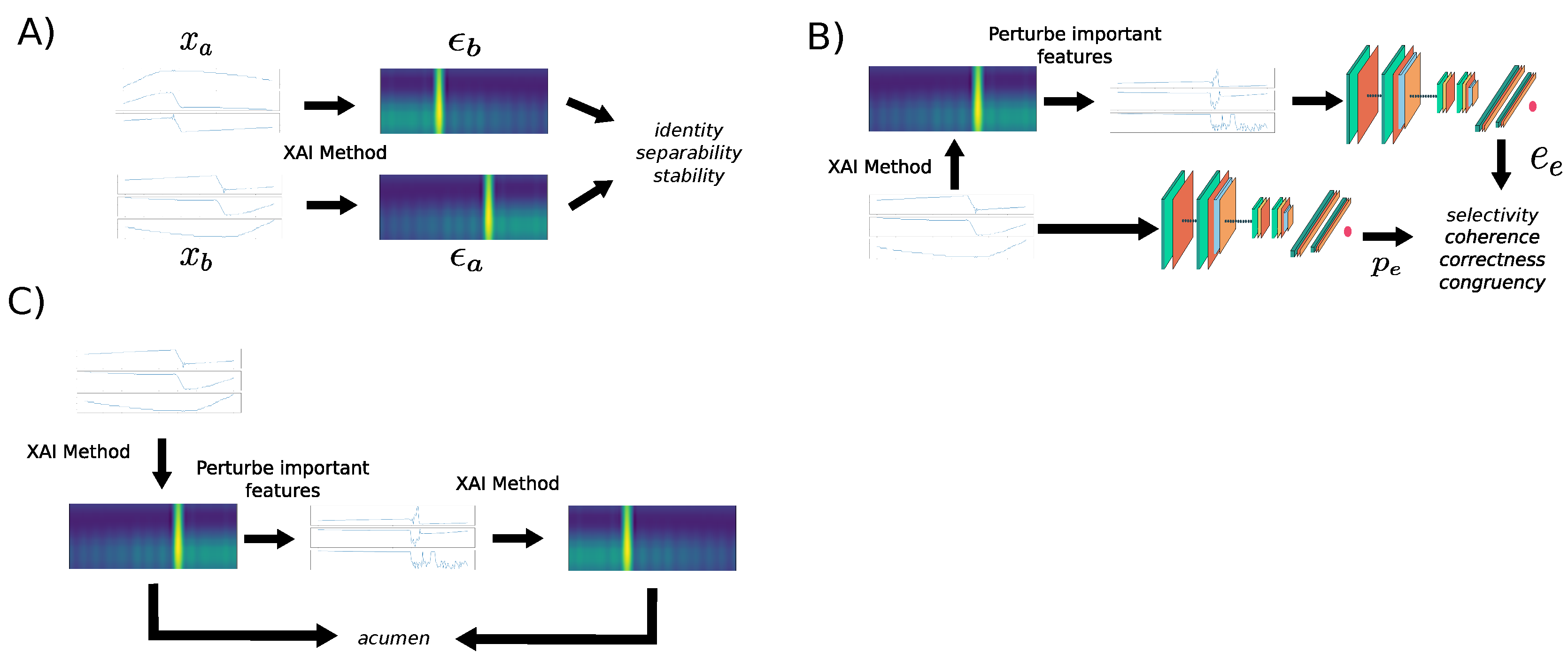
This study uses the most relevant quantitative proxies found in the literature [24,34], to evaluate and compare each method. Different methodologies need to be followed depending on the proxy used to evaluate the interpretability of machine learning models. These methodologies are depicted graphically in Figure 3. Approach A involves using different samples and their corresponding explanations to compute metrics such as identity, separability, and stability. In approach B, a specific sample is perturbed using its own explanation, and the difference in prediction errors (between the original and perturbed sample) is computed. This methodology is used to evaluate metrics such as selectivity, coherence, correctness, and congruence. Approach C involves using the explanation of the original sample to build the perturbed sample, then the explanations from both the original and perturbed samples are used to compute the acumen proxy.

The following are the desirable characteristics that each XAI method should accomplish, and the proxy used for each one in this work:

• Identity: The principle of identity states that identical objects should receive identical explanations. This estimates the level of intrinsic non-determinism in the method:

  $$\forall a,b\left(d(x_a,x_b)=0\Rightarrow d({ϵ}_a,{ϵ}_b)=0\right)$$

  (14)

  where x are samples, d is a distance function, and $ϵ$ explanation vectors (which explain the prediction of each sample).
• Separability: Non-identical objects cannot have identical explanations.

  $$\forall a,b\left(d(x_a,x_b)\ne 0\Rightarrow d({ϵ}_a,{ϵ}_b)>0\right)$$

  (15)
  If a feature is not actually needed for the prediction, then two samples that differ only in that feature will have the same prediction. In this scenario, the explanation method could provide the same explanation, even though the samples are different. For the sake of simplicity, this proxy is based on the assumption that every feature has a minimum level of importance, positive or negative, in the predictions.
• Stability: Similar objects must have similar explanations. This is built on the idea that an explanation method should only return similar explanations for slightly different objects. The Spearman correlation $\rho$ is used to define this:

  $$\rho (\left\{d(x_i,x_0),d(x_i,x_1),...,d(x_i,x_n)\right\},\left\{d({ϵ}_i,{ϵ}_0),d({ϵ}_i,{ϵ}_1),...,d({ϵ}_i,{ϵ}_n)\right\})\underset{\forall i}{=}{\rho }_i>0$$

  (16)
• Selectivity. The elimination of relevant variables must negatively affect the prediction [9,35]. To compute the selectivity, the features are ordered from the most to least relevant. One by one the features are removed, by setting it to zero for example, and the residual errors are obtained to obtain the area under the curve (AUC).
• Coherence. It computes the difference between the prediction error $p_e^i$ over the original signal and the prediction error $e_e^i$ of a new signal where the non-important features are removed.

  $${\alpha }_i=\left|p_e^i-e_e^i\right|$$

  (17)

  where ${\alpha }_i$ is the coherence of a sample.
• Completeness. It evaluates the percentage of the explanation error from its respective prediction error.

  $${\gamma }_i=\frac{e_e^i}{p_e^i}$$

  (18)
• Congruence. The standard deviation of the coherence provides the congruence proxy. This metric helps to capture the variability of the coherence.

  $$\delta =\sqrt{\frac{\sum ({({\alpha }_i-\overline{\alpha })}^2}{N}}$$

  (19)

  where $\overline{\alpha }$ is the average coherence over a set of N samples:

  $$\overline{\alpha }=\frac{\sum {\alpha }_i}{N}$$

  (20)
• Acumen. It is a new proxy proposed by the authors for the first time in this paper, based on the idea that an important feature according to the XAI method should be one of the least important after it is perturbed. This proxy aims to detect whether the XAI method depends on the position of the feature, in our case, the time dimension. It is computed by comparing the ranking position of each important feature after perturbing it.

  $$\varpi =1-\frac{{{\displaystyle \sum }_{f_i\in \mathcal{I}}}^{\frac{p_a\left(f_i\right)}{N}}}{M}$$

  (21)

  where $\mathcal{I}$ is the set of M important features before the perturbation and $p_a\left(f_i\right)$ is a function that returns the position of feature $f_i$ within the importances vector after the perturbation, where features with lower importance are located at the beginning of the vector.

Some of the previously depicted methods for evaluating the interpretability of machine learning models perturb the most important features identified by the XAI method. In our paper, we define the most important features as those whose importance values are greater than 1.5 times the standard deviation of the importance values, up to a maximum of 100 features.

3. Experiments and Results

3.1. Problem Description

The problem revolves around the development of a model h capable of predicting the remaining useful life y of the system, using a set of input variables x. The former is an optimization problem that can be denoted as:

$$\underset{h\in \mathcal{H}}{argmin}\sum \mathcal{S}\left(y-h\left(x\right)\right)$$

(22)

where y and $h\left(x\right)$ are, respectively, the expected and estimated RUL. $\mathcal{H}$ is the set of the different models to be tested by the optimization process and $\mathcal{S}$ is a scoring function defined as the average of the Root-Mean-Square Error (RMSE) and NASA’s scoring function ($N_s$) [36]:

$$\mathcal{S}=0.5·RMSE+0.5·N_s$$

(23)

$$N_s=\frac{1}{M}\sum exp\left(\alpha \right|y-\widehat{y}\left|\right)-1$$

(24)

M being the number of samples and $\alpha$ being equal to $\frac{1}{13}$ in case that $\widehat{Y}<Y$ and $\frac{1}{10}$ otherwise.

3.2. Datasets

The experiments have been carried out using three different datasets: a dataset of accelerated degradation of bearings, a dataset of commercial lithium iron phosphate/graphite cells cycled under fast-charging conditions, and a dataset of simulated run-to-failure turbofan engines. Those three datasets are focused on RUL prediction. Each of these datasets will be described below.

3.2.1. PRONOSTIA Dataset

The first dataset used is the bearing operation data collected by FEMTO-ST, a French research institute, on the PRONOSTIA platform [37]. Figure 4 shows a diagram of the platform and the sensors used to collect data on it. To gather the data, three operating conditions were used to accelerate the degradation of the bearings: 1800 rpm of rotating speed with 4000 N of payload weight, 1650 rpm and 4200 N, and 1500 rpm and 5000 N.

They employed two sensors, set in the x-axis and y-axis of the bearing. The data were acquired every 10 s for 0.1 s, with a frequency of 25.6 kHz. Therefore, each time series has 2560 data points. The experiment was stopped when the vibration amplitude exceeded the threshold of 20 g. It is assumed that the remaining useful life (RUL) will decrease linearly from the maximum value (total time of the experiment) to 0. For this experiment, the RUL is normalized to be between 0 and 1. Figure 5 shows the two full history signals of one of the bearings.

To train the network, inputs are generated taking random windows of 256 data points during the 0.1 s sampling period. The RUL is computed as $\frac{t_{end}-t_{sample}}{t_{end}}$, where $t_{end}$ is the total time of the experiment and $t_{sample}$ is the time of the treated sample. The vertical and horizontal sensor values are normalized by dividing them by 50, as the range of values of the sensors is $[-50,50]$. To train the network, bearings 1, 3, 4, and 7 are selected, while bearings 2, 5, and 6 are used in the test set.

3.2.2. Fast-Charging Catteries

Severson et al. [38] recently made available a large public dataset of 124 LFP-graphite cells. These cells underwent cycles to 80% of their initial capacities under various fast-charging conditions ranging from 3.6 to 6 C in an environmental chamber at 30 °C. Subsequently, the cells were charged from 0% to 80% SOC using one-step or two-step charging profiles. All cells were then charged from 80% to 100% SOC to 3.6 V and discharged to 2.0 V, with the cut-off current set to C/50. During the cycling test, the cell temperature was recorded and the internal resistance was obtained at 80% SOC.

The entire dataset is made up of three batches, but for this paper, only the first batch is used, which consists of 47 battery experiments. Fifteen of these experiments were used to test the model, while the remaining experiments were used for training. Nine features were used to train the model, with a window of 256 data points taken from each charging or discharging cycle.

The RUL is calculated using the formula $t_{end}-t_{sample}$, where $t_{end}$ is the total time of the experiment in cycles and $t_{sample}$ is the current cycle of the analyzed sample. The input features are scaled between 0 and 1 by computing the minimum and maximum values from the training samples, which are then used to scale both the training and testing datasets.

3.2.3. N-CMAPSS Dataset

The Commercial Modular Aero-Propulsion System Simulation (CMAPSS) is a modeling software developed at NASA. It was used to build the well known CMAPSS dataset [36] as well as the recently created N-CMAPSS dataset [39]. N-CMAPSS was created providing the full history of the trajectories starting with a healthy condition until the failure occurs. A schematic of the turbofan model used in the simulations is shown in Figure 6. All rotation components of the engine (fan, LPC, HPC, LPT, and HPT) can be affected by the degradation process.

Seven different failure modes, related to flow degradation or subcomponent efficiency, that can be present in each flight have been defined. The flights are divided into three classes depending on the length of the flight. Flights with a duration from 1 to 3 h belong to class 1, class 2 consists of flights between 3 and 5 h, and flights that take more than 5 h fall into class 3. Each flight is divided into cycles, covering climb, cruise, and descend operations.

The input variables used are the sensor outputs $x_s$, the scenario descriptors w, and auxiliary data a. The different variables available to estimate the RUL of the system are described in

Table 1. Variable description, symbol, units and variable set.

Symbol	Set	Description	Units
alt	W	Altitude	ft
Mach	W	Flight Mach number	-
TRA	W	Throttle-resolver angle	%
T2	W	Total temperature at fan inlet	°R
Wf	$X_s$	Fuel flow	pps
Nf	$X_s$	Physical fan speed	rpm
Nc	$X_s$	Physical core speed	rpm
T24	$X_s$	Total temperature at LPC outlet	°R
T30	$X_s$	Total temperature at HPC outlet	°R
T48	$X_s$	Total temperature at HPT outlet	°R
T50	$X_s$	Total temperature at LPT outlet	°R
P15	$X_s$	Total pressure in bypass-duct	psia
P2	$X_s$	Total pressure at fan inlet	psia
P21	$X_s$	Total pressure at fan outlet	psia
P24	$X_s$	Total pressure at LPC outlet	psia
Ps30	$X_s$	Static pressure at HPC outlet	psia
P40	$X_s$	Total pressure at burner outlet	psia
P50	$X_s$	Total pressure at LPT outlet	psia
Fc	A	Flight class	-
$h_s$	A	Health state	-

.

The model used in the experimentation was designed and implemented by the authors and it received third place in the 2021 PHM Conference Data Challenge [40]. The former 20 variables have different scales, thus a z-score normalization is applied to homogenize the variables scale:

$$x_f^{\prime }=\frac{x_f-{\mu }_f}{{\sigma }_f}$$

(25)

where $x_f$ is the data of a feature f, and ${\mu }_f$ and ${\sigma }_f$ are their mean and standard deviation, respectively.

The network inputs are generated by sliding a time window through the normalized data, with the window size denoted as $L_w$ and determined during model selection. The inputs are defined as

$$X_t^k=[{\tilde{\mathcal{X}}}_{t_{end}-L_w}^k,\dots ,{\tilde{\mathcal{X}}}_{t_{end}}^k]$$

where $t_{end}$ is the end time of the window (see Figure 7). The corresponding ground truth RUL label for each input is denoted as $Y_t$. This method generates $T^k-L_w$ samples for each unit, where $T^k$ represents the total run time in seconds of the unit.

The ground-RUL label has been defined as a linear function of cycles from the RUL of each unit $Y_t^k=TU{L}^k-C_t^k$, where $TU{L}^k$ is the total useful life of the unit k in cycles and $C_t^k$ is the number of past cycles from the beginning of the experiment at time t.

3.3. The Black-Box Models

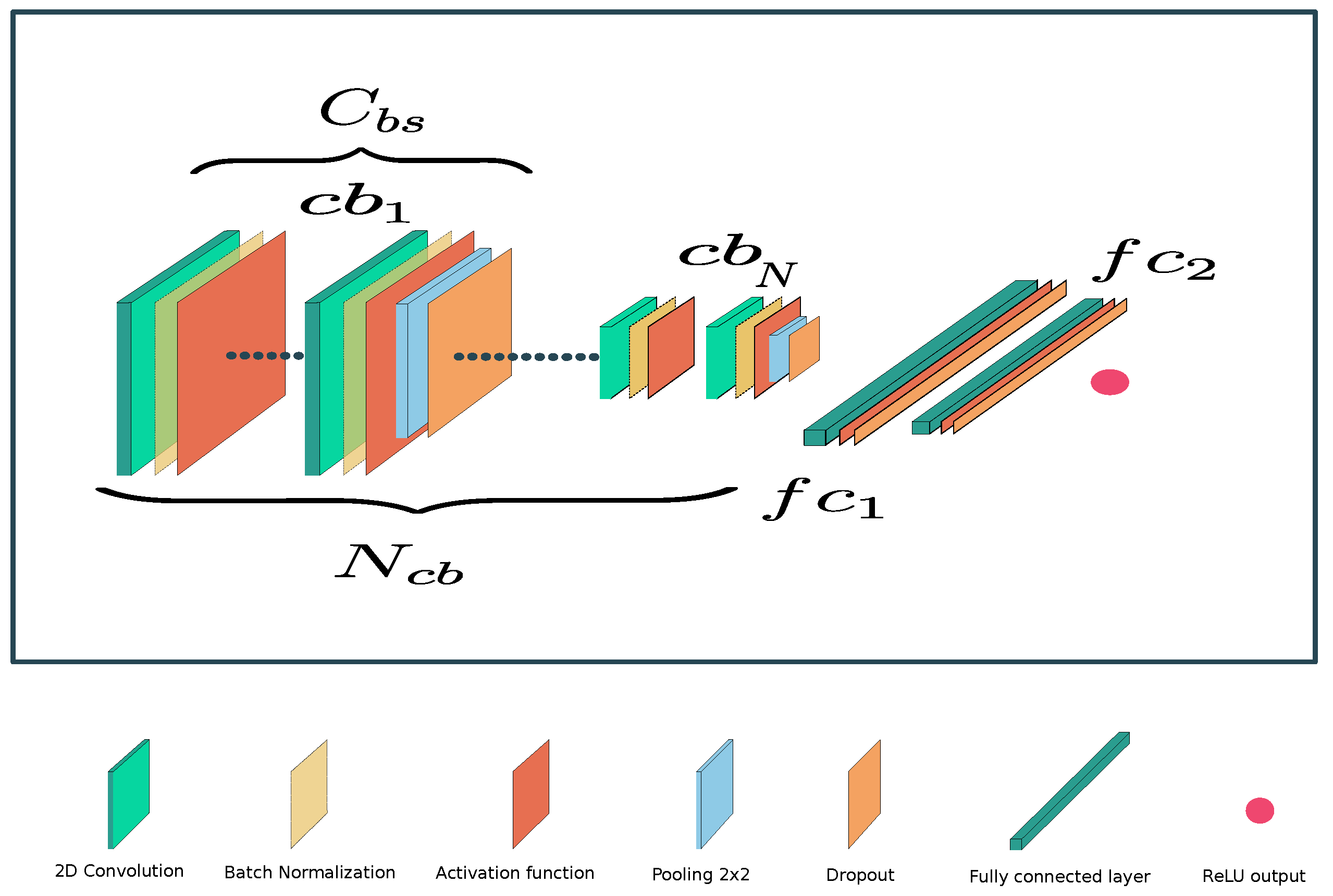
The black-box models are all a Deep Convolutional Neural Network (DCNN). The classical DCNN architecture, which is shown in Figure 8, can be divided into two parts. The first part consists of a stacking of $N_b$ blocks, each of which consists of $C_{bs}$ stacked sub-blocks that include convolutional and pooling layers. The main objective of this part is to extract relevant features for the task at hand. The second part is made up of two fully connected layers, which are responsible for performing the regression of the RUL. The output layer uses the rectified linear unit (ReLU) activation function, since negative values in the output are not desired. The detailed parameters of the networks can be found in

Table 2. Parameters of the black-box model developed.

Parameter	PRONOSTIA	N-CMAPSS	Fast Charge
$L_w$	256	161	512
$B_s$	32	116	32
$C_{bs}$	2	4	3
$N_{cb}$	4	4	3
$f{c}_1$	118	256	168
$f{c}_2$	100	100	24
$kernelsize$	(1, 10)	(3, 3)	(1, 10)
${\sigma }_{conv}$	ReLU	tanh	ReLU
$d_{rate}$	4	2	4
${\sigma }_{fc}$	ReLU	Leaky ReLU	tanh
${\sigma }_{output}$	ReLU	ReLU	ReLU
Net params	$3.0\times {10}^6$	$1.5\times {10}^6$	$2.8\times {10}^6$
RMSE	0.24	10.46	84.78
MAE	0.17	7.689	51.98
NASA score	0.015	2.13	-
CV $\mathcal{S}$ score	-	6.30	-
std($\mathcal{S}$)	-	0.37	-

.

While it is possible that these architectures could be considered simple from the perspective of the current state-of-the-art in deep learning, they are still complex enough to not be directly interpretable models. Thus, they are still valuable for achieving the goals of this paper. Other models such as recurrent networks and transformers can be used for time-series analysis. However, applying some of the model-specific XAI methods studied in this paper can be challenging due to the accumulation of information within recurrent cells or the self-attention mechanism of transformers. In these cases, other methods such as attention mechanisms may be more commonly used to extract explanations and interpret how the model processes the time-series data.

3.4. Experiments

The experiments were conducted using sets of 256 data samples for each dataset. These samples were not used during the model training phase. The 8 proxies, that were defined in Section 2.3, were computed for each sample, and the final score for each proxy was determined by taking the mean of the 256 samples as described in the Algorithm 1. This process was repeated for each XAI method studied.

For both LIME and SHAP, five perturbation methods were tested: zero, one, mean, uniform noise, and normal noise. In the case of selectivity, due to performance issues, groups of 10 features, ordered by importance, were considered for computing the AUC. The number of samples used to train the surrogate model in LIME and SHAP was selected as 1000 to ensure reasonably good performance of the linear model and acceptable time performance. However, these two methods are 10 times slower than the rest.

Algorithm 1 Algorithm to compute each proxy on the test set

X is a set of N samples P is a proxy $N\leftarrow \left|X\right|$ $S\leftarrow 0$ for$x_i\in X$do       $s_i\leftarrow P\left(x_i\right)$       $S\leftarrow S+s_i$ end for return$$

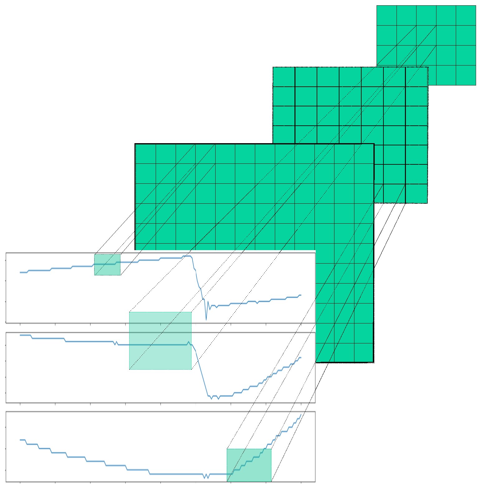
For the remaining XAI methods, the replace-by-zero perturbation method has been used since, in the experiments performed, it provided the best results. Finally, in Grad-CAM, different values between 0 and 1 for $\beta$ and $\sigma$ (factors adjusting the contribution of the time and feature components in the computation of feature importance) were tested using a grid search methodology with a step of 0.1. Furthermore, heat maps were extracted for each convolutional layer to study the best layer for explaining the predictions of the DCNN model on this dataset. It is important to note that the gradients are distributed differently depending on its depth within the network (Figure 9), which means that the last convolutional layer, commonly exploited in the literature, may not be the best to solve all problems. By using the proxies, it is possible to assess which is the best layer from the perspective of explainability.

3.5. Results

The results for each method are presented in

Table 3. This table shows the result of different proxies for the PRONOSTIA dataset. Perm: Permutation, I: Identity, Sep: Separability, Sel: Selectivity, Sta: Stability, Coh: Coherence, Comp: Completeness, Cong: Congruence, Acu: Acumen. The maximum value for each proxy has been highlighted in bold.

Method	Perm	I	Sep	Sta	Sel	Coh	Comp	Cong	Acu	Total
SHAP	mean	0.0	1.000	−0.009	0.533	0.054	0.989	0.105	0.495	0.382
SHAP	n.noise	0.0	1.000	0.020	0.532	0.053	0.991	0.103	0.485	0.386
SHAP	u.noise	0.0	1.000	0.078	0.521	0.032	0.994	0.084	0.487	0.387
SHAP	zero	0.0	1.000	0.011	0.529	0.012	0.997	0.045	0.519	0.371
SHAP	one	1.0	1.000	−0.015	0.528	0.093	0.997	0.128	0.402	0.533
GradCAM		1.0	0.976	0.368	0.531	0.141	0.980	0.134	0.206	0.542
LRP		0.0	1.000	0.042	0.536	0.158	0.970	0.133	0.502	0.406
Saliency		1.0	1.000	−0.122	0.544	0.155	0.975	0.131	0.180	0.526
Lime	mean	0.0	1.000	0.038	0.538	0.040	0.986	0.081	0.553	0.383
Lime	n.noise	0.0	1.000	0.034	0.538	0.042	0.985	0.083	0.537	0.383
Lime	u.noise	0.0	1.000	−0.043	0.530	0.032	0.985	0.071	0.525	0.368
Lime	zero	1.0	1.000	0.108	0.529	0.008	1.004	0.036	0.500	0.526
Lime	one	1.0	1.000	0.016	0.540	0.052	0.992	0.101	0.435	0.529

,

Table 4. This table shows the result of different proxies for the fast-charging batteries dataset. Perm: Permutation, I: Identity, Sep: Separability, Sel: Selectivity, Sta: Stability, Coh: Coherence, Comp: Completeness, Cong: Congruence, Acu: Acumen. The maximum value for each proxy has been highlighted in bold.

Method	Perm	I	Sep	Sta	Sel	Coh	Comp	Cong	Acu	Total
SHAP	mean	0.000	1.000	0.119	0.584	0.097	0.903	0.121	0.418	0.405
SHAP	n.noise	0.000	1.000	0.120	0.588	0.100	0.900	0.122	0.383	0.402
SHAP	u.noise	0.000	1.000	0.180	0.616	0.107	0.893	0.121	0.303	0.403
SHAP	zero	1.000	1.000	0.153	0.597	0.093	0.908	0.130	0.536	0.552
SHAP	one	1.000	1.000	0.176	0.526	0.077	0.923	0.113	0.269	0.510
LRP		0.441	1.000	0.007	0.659	0.073	0.936	0.076	0.492	0.460
GradCAM		1.000	1.000	0.259	0.664	0.063	1.050	0.080	0.317	0.554
Saliency		1.000	0.990	0.163	0.517	0.170	0.831	0.157	0.452	0.535
Lime	mean	0.023	1.000	0.456	0.595	0.087	0.913	0.116	0.501	0.461
Lime	n.noise	0.023	1.000	0.447	0.598	0.087	0.914	0.115	0.529	0.464
Lime	u.noise	0.027	0.999	0.333	0.632	0.102	0.899	0.114	0.227	0.417
Lime	zero	1.000	1.000	0.512	0.608	0.221	0.781	0.156	0.296	0.572
Lime	one	1.000	1.000	0.601	0.537	0.065	0.936	0.061	0.138	0.542

and

Table 5. This table shows the result of different proxies for the N-CMAPSS dataset. Perm: Permutation, I: Identity, Sep: Separability, Sel: Selectivity, Sta: Stability, Coh: Coherence, Comp: Completeness, Cong: Congruence, Acu: Acumen. The maximum value for each proxy has been highlighted in bold.

Method	Perm	I	Sep	Sta	Sel	Coh	Comp	Cong	Acu	Total
SHAP	mean	0.000	1.000	0.033	0.582	0.120	0.973	0.152	0.505	0.421
SHAP	n.noise	0.000	1.000	0.037	0.581	0.116	0.968	0.150	0.501	0.419
SHAP	u.noise	0.000	1.000	0.027	0.581	0.125	0.961	0.162	0.503	0.420
SHAP	zero	1.000	1.000	0.226	0.800	0.152	1.010	0.149	0.761	0.637
SHAP	one	1.000	1.000	0.200	0.692	0.173	0.969	0.169	0.349	0.569
GradCAM		1.000	1.000	0.653	0.702	0.196	0.948	0.170	0.435	0.638
LRP		1.000	1.000	−0.037	0.599	0.180	0.967	0.165	0.495	0.546
Saliency		1.000	0.999	0.055	0.434	0.174	0.972	0.163	0.516	0.539
Lime	mean	0.004	1.000	0.130	0.569	0.173	0.962	0.161	0.685	0.461
Lime	n.noise	0.008	1.000	0.131	0.572	0.173	0.960	0.162	0.677	0.460
Lime	u.noise	0.012	1.000	0.109	0.560	0.166	0.960	0.162	0.577	0.443
Lime	zero	1.000	1.000	0.554	0.835	0.160	1.017	0.146	0.753	0.683
Lime	one	1.000	1.000	0.349	0.728	0.184	0.969	0.166	0.069	0.558

.

For the model trained with the PRONOSTIA dataset, Grad-CAM obtained the highest results for three out of the eight proxies tested, and for selectivity, completeness, and coherence, the values were close to the maximum. When the average results for each method were considered, Grad-CAM achieved the best overall performance. The optimal result for Grad-CAM was obtained using $\beta =0.5$, $\sigma =0.5$, and computing the gradient with respect to the third layer of the network.

For the model trained with the fast-charging batteries dataset, Grad-CAM achieved the highest results in four out of the eight proxies. In this case, the scores obtained for coherence and congruence are bad; they are almost 50 percent lower than the best result obtained by LIME and Saliency respectively. The network layer that achieved the best results was the first layer with $\beta =0.5$, $\sigma =0.9$.

Regarding the model trained with the N-CMAPSS dataset, the table indicates that Grad-CAM achieved the highest value for five out of the eight proxies tested, and for selectivity and completeness, the values were close to the maximum. The optimal result for Grad-CAM was obtained using $\beta =0.9$, $\sigma =0.0$, and computing the gradient with respect to the second layer of the network.

It is interesting to note that the optimal values for the hyperparameters $\beta$ and $\sigma$ were different for the different models. This highlights the importance of tuning these parameters to the specific characteristics of the dataset and the model being used.

Note that, among all the proxies considered in this work to assess the quality and consistency of XAI methods explanations, Grad-CAM achieves the worst result when evaluated using the acumen proxy, defined in this work.

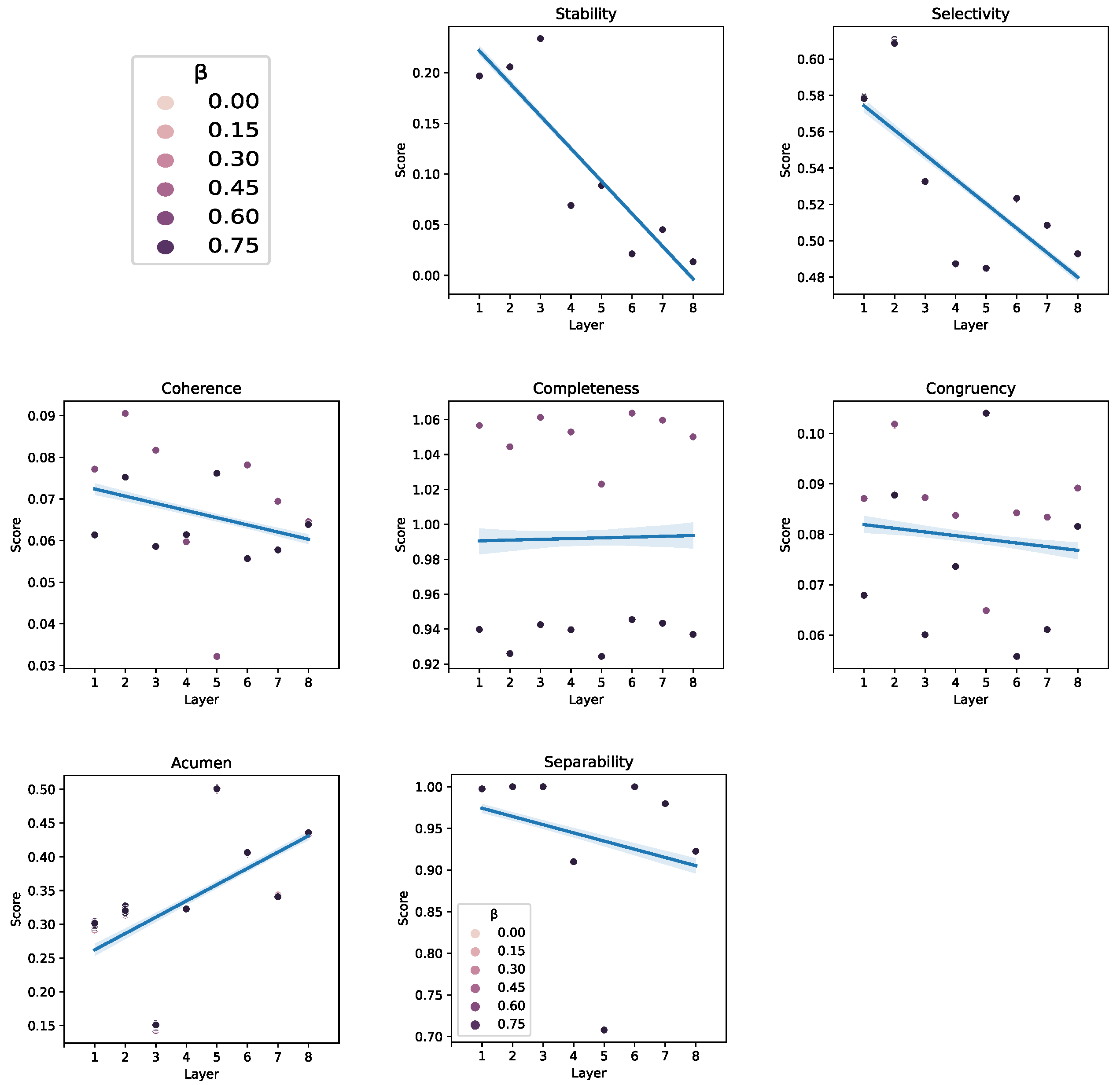
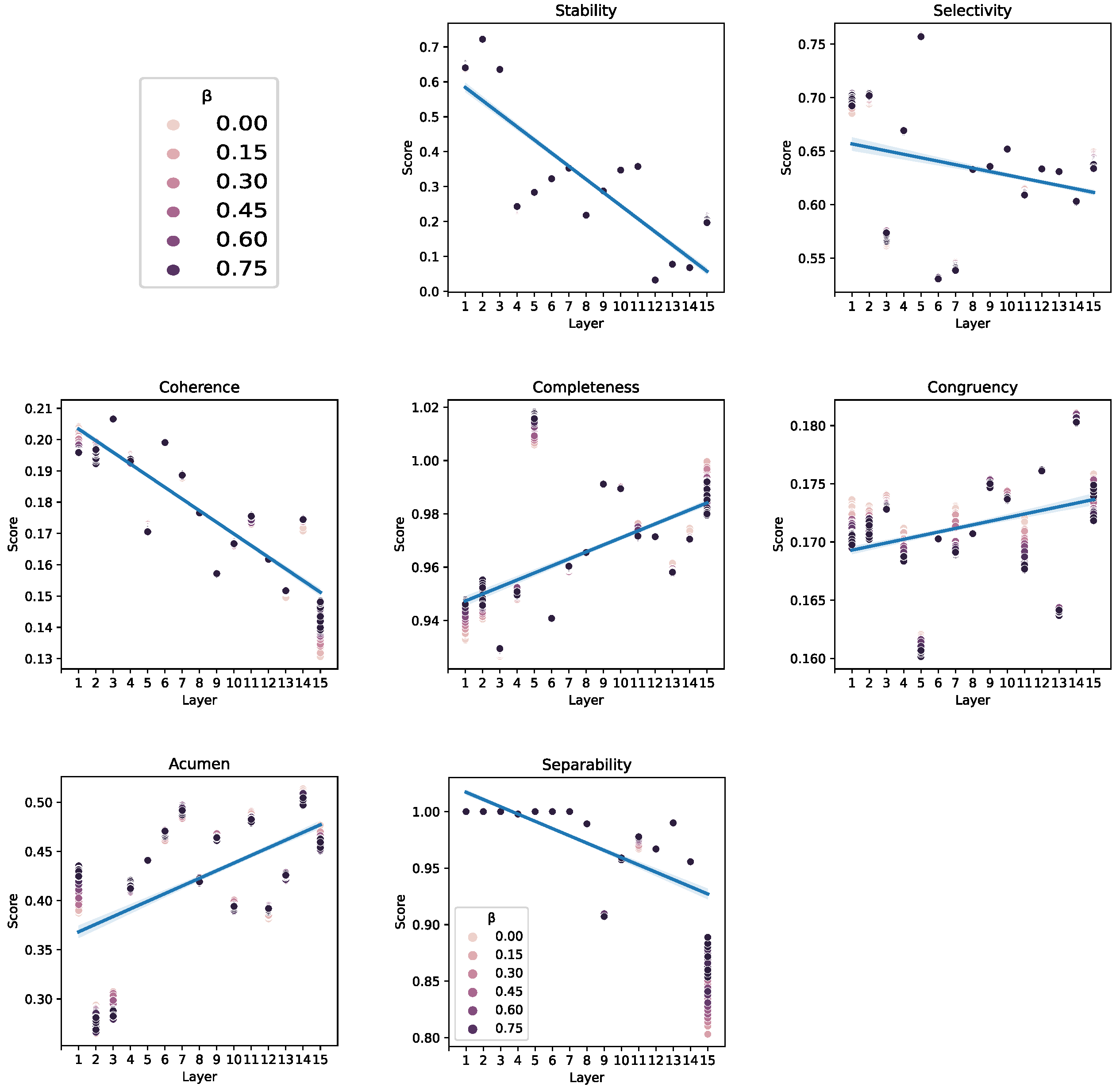
Since Grad-CAM tends to produce the best results in a few of the proxies, it is considered the more robust method. Further analysis has been carried out to understand the behavior of the method under different settings for each of the studied proxies, with the exception of the identity proxy, which is always 1 in Grad-CAM. Figure 10, Figure 11 and Figure 12 compare the scores obtained by Grad-CAM when applied to each convolutional layer of the DCNN.

Table 6. This table shows the kind of correlations of each proxy with the depth of the layer in the network. Sep: Separability, Sel: Selectivity, Sta: Stability, Coh: Coherence, Comp: Completeness, Cong: Congruence, Acu: Acumen.

	Sta	Sel	Coh	Comp	Con	Acu	Sep
PRONOSTIA	I	I	-	-	D	-	-
Fast-charging batteries	I	I	I	-	I	D	I
N-CMAPSS	I	I	I	D	D	D	I

summarizes the kind of correlation of each proxy with the depth of the layer in the network. The selectivity, stability, separability, and coherence proxies tend to have an inverse correlation with respect to the depth of the layer. Conversely, the acumen proxy presents a direct correlation with the layer depth.

The inverse correlation may be due to the existence of large groups of features having a higher likelihood of including features that impact the proxy negatively. For example, in the case of selectivity, a group that is considered important as a whole could contain samples with low importance. Therefore, for these proxies it is better to consider features independently, instead of as a group.

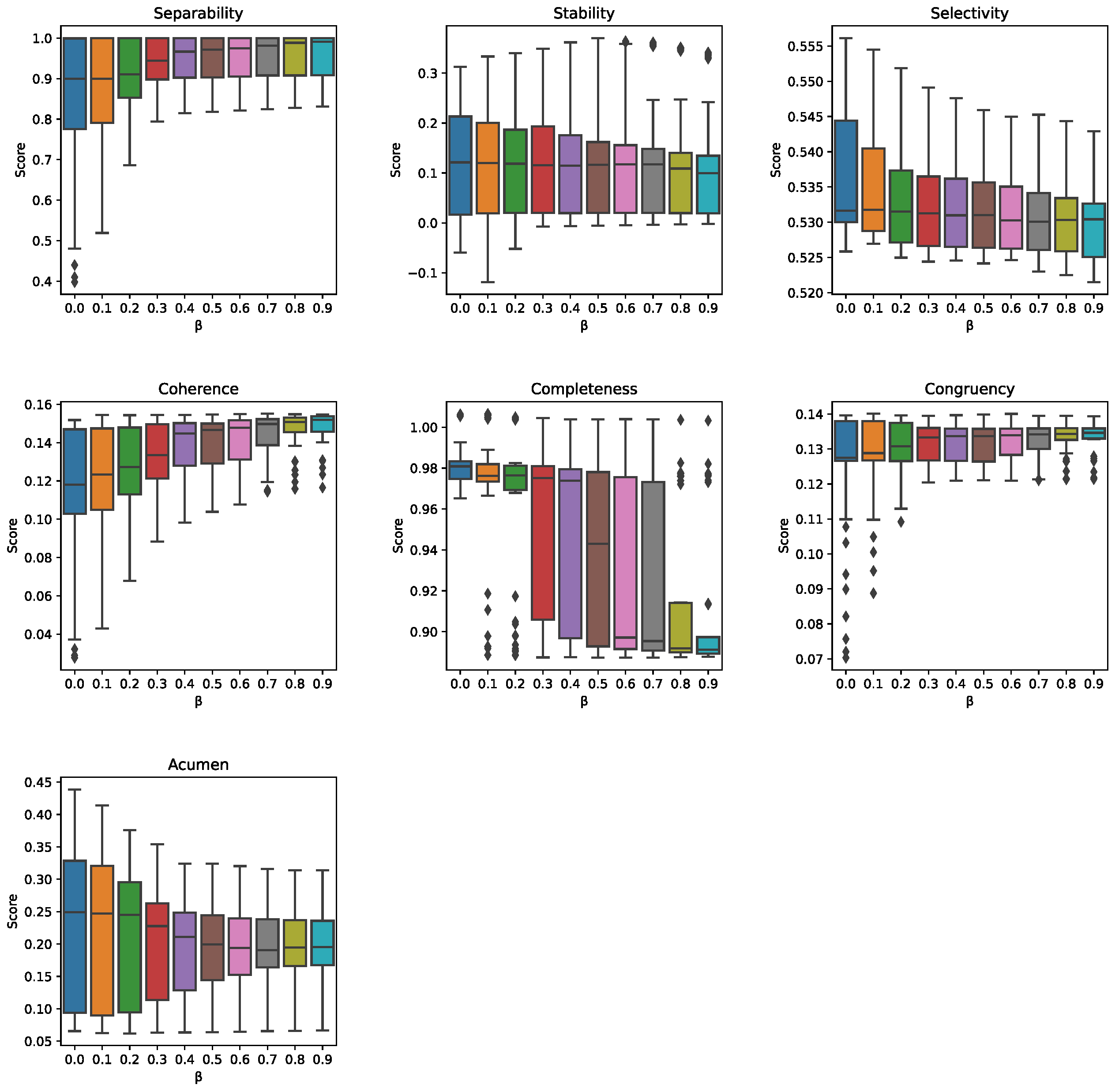
Figure 13 shows the influence of the time contribution, which is controlled by the factor $\beta$. The factor being discussed shows a direct correlation with all proxies except completeness, selectivity, and acumen, which exhibit an inverse correlation. In general, it can be concluded that increasing the weight of the time dimension in Grad-CAM could be beneficial for explainability in time-series for RUL.

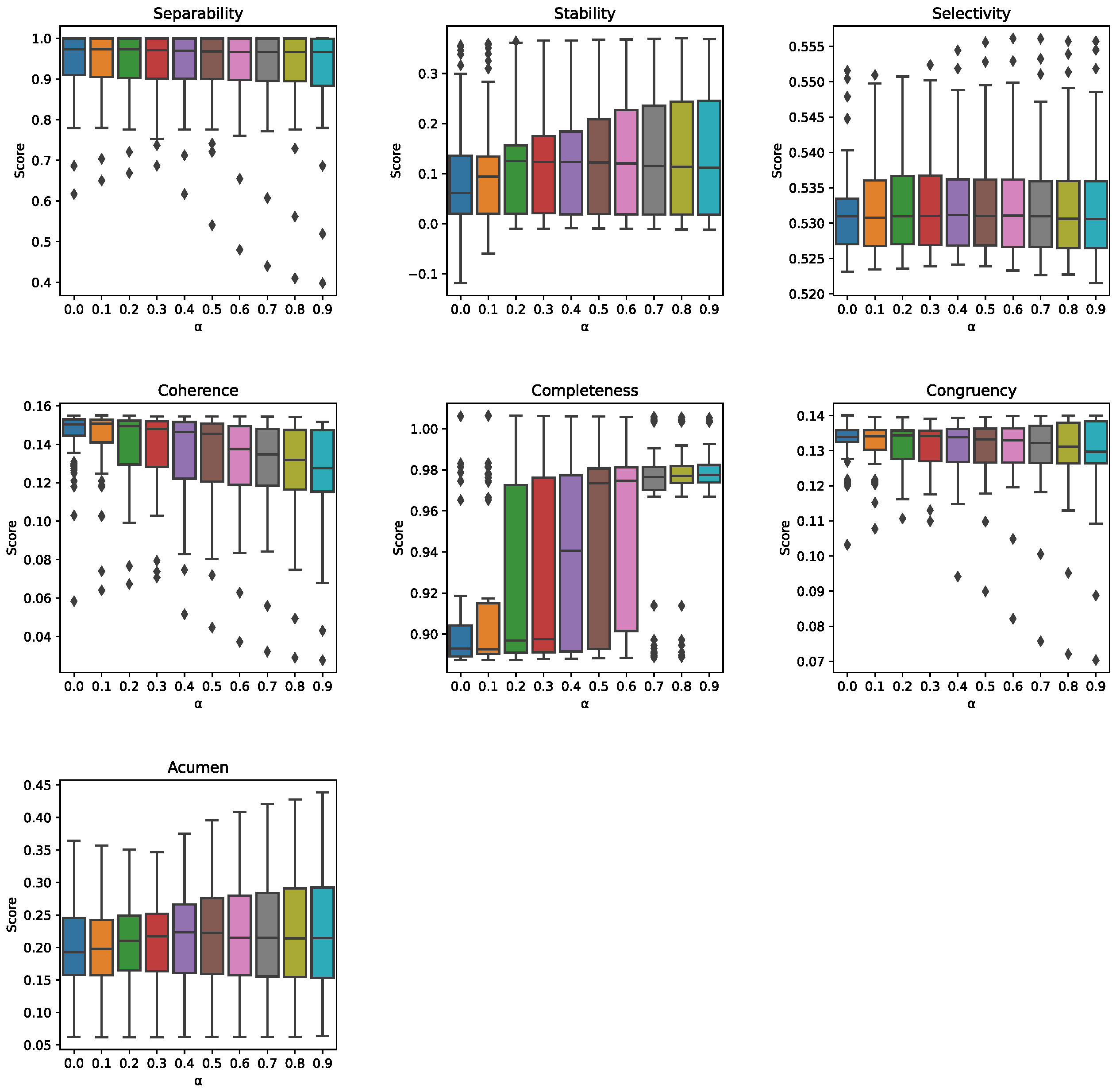
On the other hand, Figure 14 shows the influence of the feature contribution. In this case, the trend is less clear, except for completeness, which presents a strong direct correlation.

4. Discussion

This paper is focused on the under-researched area of XAI methods for time series and regression problems. The first aim of this paper was to review existing papers on XAI addressing such topics, with an emphasis on the use of quantitative metrics to compare XAI methods. Then, a comparison among the most promising XAI methods was carried out on a highly complex model, as is the DCNN, applied to time series regression problems within the context of PHM. With this aim, a number of experiments were performed, quantifying the quality of explanations, provided by the XAI methods, by computing eight different proxies. Results showed that Grad-CAM was the most robust XAI method among the ones tested, achieving the highest values for a few of the eight proxies and being close to the maximum in two others in the three experiments carried out.

In addition to comparing various XAI methods through quantitative proxies, this paper also makes two additional contributions: First, by introducing a new quantitative proxy called acumen, which measures a desirable property of any XAI method and highlights the breach of this property by Grad-CAM. Second, by proposing an extension of Grad-CAM that takes into account time and attribute dependencies (where such contributions can be modulated). Results showed that this extension improves the performance of Grad-CAM in all of the studied experiments. This is achieved thanks to the ability to adapt Grad-CAM to the nature of the different datasets by adjusting the contribution of the time and attribute dependencies (by means of $\beta$ and $\sigma$ parameters).

The results also showed that the impact of the layers and the time component contribution $\beta$ on Grad-CAM varied for different proxies, showing for some of them a direct correlation and for others an inverse correlation. These findings demonstrate the importance of considering time and attribute dependencies when evaluating the performance of XAI methods in time series and provide valuable insights for future research in this area.

The results of this study highlight the need for further research in this area and the importance of developing better XAI methods for time series and regression problems, particularly in the PHM field.

The experiments were carried out using deep neural networks trained to predict the remaining useful life of various datasets, which belongs to a type of regression problem that has received little attention in XAI. All the code to reproduce the experiments, along with the data and the model, is provided to allow the research community to further explore these findings. Overall, this paper makes a valuable contribution to the field of XAI by addressing important gaps in the literature and presenting novel approaches for time series and regression problems.

5. Future Work

There are several potential directions for future research in the area of XAI for RUL in time-series.

First, it would be interesting to explore the use of XAI methods on recurrent neural networks (RNNs), transformer-based architectures, and other more complex neural network architectures such as ResNet or DenseNet for RUL prediction tasks. Recurrent neural networks (RNNs) and transformer-based models have shown great success in capturing sequential and long-term dependencies, which are crucial for RUL prediction tasks that involve time-series data. Therefore, the study of which XAI methods, including attention mechanisms among others, work better in these architectures could be valuable for the research community.

Second, an interesting avenue for future research is the composition of layers with Grad-CAM. This work has shown insight into the fact that the depth of the layer is dependent for some proxies. Therefore, optimizing the contribution of a few layers could improve the score of the proxies capturing different aspects of the signal.

Overall, future work in this area should focus on developing more effective and interpretable models or methods that can provide insight into not only the part of the signal responsible for the prediction, but also the specific characteristics of the signal. This will enable domain experts to make informed decisions based on the model’s outputs more easily and effectively.

References

1. Pomerleau, D.A. Neural networks for intelligent vehicles. In Proceedings of the IEEE Conference on Intelligent Vehicles, Tokyo, Japan, 14–16 July 1993; pp. 19–24. [Google Scholar]
2. Goodman, B.; Flaxman, S. European Union regulations on algorithmic decision-making and a “right to explanation”. AI Mag. 2017, 38, 50–57. [Google Scholar] [CrossRef] [Green Version]
3. Gilpin, L.H.; Bau, D.; Yuan, B.Z.; Bajwa, A.; Specter, M.; Kagal, L. Explaining explanations: An overview of interpretability of machine learning. In Proceedings of the 2018 IEEE 5th International Conference on Data Science and Advanced Analytics (DSAA), Turin, Italy, 1–3 October 2018; pp. 80–89. [Google Scholar]
4. Arrieta, A.B.; Díaz-Rodríguez, N.; Del Ser, J.; Bennetot, A.; Tabik, S.; Barbado, A.; García, S.; Gil-López, S.; Molina, D.; Benjamins, R.; et al. Explainable Artificial Intelligence (XAI): Concepts, taxonomies, opportunities and challenges toward responsible AI. Inf. Fusion 2020, 58, 82–115. [Google Scholar] [CrossRef] [Green Version]
5. Ribeiro, M.T.; Singh, S.; Guestrin, C. “Why should I trust you?” Explaining the predictions of any classifier. In Proceedings of the 22nd ACM SIGKDD International Conference on Knowledge Discovery and Data Mining, San Francisco, CA, USA, 13–17 August 2016; pp. 1135–1144. [Google Scholar]
6. Lundberg, S.M.; Lee, S.-I. A unified approach to interpreting model predictions. In Advances in Neural Information Processing Systems; MIT Press: Cambridge, MA, USA, 2017; Volume 30, pp. 4768–4777. [Google Scholar]
7. Selvaraju, R.R.; Cogswell, M.; Das, A.; Vedantam, R.; Parikh, D.; Batra, D. Grad-cam: Visual explanations from deep networks via gradient-based localization. In Proceedings of the IEEE International Conference on Computer Vision, Venice, Italy, 22–29 October 2017; pp. 618–626. [Google Scholar]
8. Simonyan, K.; Vedaldi, A.; Zisserman, A. Deep inside convolutional networks: Visualising image classification models and saliency maps. In Proceedings of the 2nd International Conference on Learning Representations (ICLR), Banff, AB, Canada, 14–16 April 2014. [Google Scholar]
9. Bach, S.; Binder, A.; Montavon, G.; Klauschen, F.; Müller, K.-R.; Samek, W. On pixel-wise explanations for non-linear classifier decisions by layer-wise relevance propagation. PLoS ONE 2015, 10, e0130140. [Google Scholar] [CrossRef] [PubMed] [Green Version]
10. Letzgus, S.; Wagner, P.; Lederer, J.; Samek, W.; Müller, K.-R.; Montavon, G. Toward Explainable AI for Regression Models. IEEE Signal Process. Mag. 2022, 39, 40–58. [Google Scholar] [CrossRef]
11. Schlegel, U.; Arnout, H.; El-Assady, M.; Oelke, D.; Keim, D.A. Towards a rigorous evaluation of xai methods on time series. In Proceedings of the 2019 IEEE/CVF International Conference on Computer Vision Workshop (ICCVW), Seoul, Republic of Korea, 27–28 October 2019; pp. 4197–4201. [Google Scholar]
12. Siddiqui, S.A.; Mercier, D.; Munir, M.; Dengel, A.; Ahmed, S. Tsviz: Demystification of deep learning models for time-series analysis. IEEE Access 2019, 7, 67027–67040. [Google Scholar] [CrossRef]
13. Ahmed, I.; Kumara, I.; Reshadat, V.; Kayes, A.S.M.; van den Heuvel, W.J.; Tamburri, D.A. Travel Time Prediction and Explanation with Spatio-Temporal Features: A Comparative Study. Electronics 2021, 11, 106. [Google Scholar] [CrossRef]
14. Vijayan, M.; Sridhar, S.S.; Vijayalakshmi, D. A Deep Learning Regression Model for Photonic Crystal Fiber Sensor with XAI Feature Selection and Analysis. IEEE Trans. NanoBiosci. 2022. [Google Scholar] [CrossRef] [PubMed]
15. Mamalakis, A.; Barnes, E.A.; Ebert-Uphoff, I. Carefully choose the baseline: Lessons learned from applying XAI attribution methods for regression tasks in geoscience. Artif. Intell. Earth Syst. 2023, 2, e220058. [Google Scholar] [CrossRef]
16. Cohen, J.; Huan, X.; Ni, J. Shapley-based Explainable AI for Clustering Applications in Fault Diagnosis and Prognosis. arXiv 2023, arXiv:2303.14581. [Google Scholar]
17. Brusa, E.; Cibrario, L.; Delprete, C.; Di Maggio, L.G. Explainable AI for Machine Fault Diagnosis: Understanding Features’ Contribution in Machine Learning Models for Industrial Condition Monitoring. Appl. Sci. 2023, 13, 2038. [Google Scholar] [CrossRef]
18. Kratzert, F.; Herrnegger, M.; Klotz, D.; Hochreiter, S.; Klambauer, G. NeuralHydrology—Interpreting LSTMs in hydrology. In Explainable AI: Interpreting, Explaining and Visualizing Deep Learning; Springer Nature: Berlin/Heidelberg, Germany, 2019; pp. 347–362. [Google Scholar]
19. Zhang, L.; Chang, X.; Liu, J.; Luo, M.; Li, Z.; Yao, L.; Hauptmann, A. TN-ZSTAD: Transferable Network for Zero-Shot Temporal Activity Detection. IEEE Trans. Pattern Anal. Mach. Intell. 2023, 45, 3848–3861. [Google Scholar] [CrossRef] [PubMed]
20. Radford, A.; Kim, J.W.; Hallacy, C.; Ramesh, A.; Goh, G.; Agarwal, S.; Sutskever, I. Learning transferable visual models from natural language supervision. In Proceedings of the International Conference on Machine Learning, Virtual, 18–24 July 2021; pp. 8748–8763. [Google Scholar]
21. Carvalho, D.V.; Pereira, E.d.M.; Cardoso, J.S. Machine learning interpretability: A survey on methods and metrics. Electronics 2019, 8, 832. [Google Scholar] [CrossRef] [Green Version]
22. Vollert, S.; Atzmueller, M.; Theissler, A. Interpretable Machine Learning: A brief survey from the predictive maintenance perspective. In Proceedings of the 2021 26th IEEE International Conference on Emerging Technologies and Factory Automation (ETFA), Vasteras, Sweden, 7–10 September 2021; pp. 1–8. [Google Scholar]
23. Samek, W.; Wiegand, T.; Müller, K.-R. Explainable artificial intelligence: Understanding, visualizing and interpreting deep learning models. arXiv 2017, arXiv:1708.08296. [Google Scholar]
24. Honegger, M. Shedding Light on Black Box Machine Learning Algorithms: Development of an Axiomatic Framework to Assess the Quality of Methods that Explain Individual Predictions. arXiv 2018, arXiv:1808.05054. [Google Scholar]
25. Doshi-Velez, F.; Kim, B. Towards a rigorous science of interpretable machine learning. arXiv 2017, arXiv:1702.08608. [Google Scholar]
26. Silva, W.; Fernandes, K.; Cardoso, M.J.; Cardoso, J.S. Towards complementary explanations using deep neural networks. Understanding and Interpreting Machine Learning in Medical Image Computing Applications. In Proceedings of the MICCAI 2018, Granada, Spain, 16–20 September 2018; pp. 133–140. [Google Scholar]
27. Hong, C.W.; Lee, C.; Lee, K.; Ko, M.-S.; Hur, K. Explainable Artificial Intelligence for the Remaining Useful Life Prognosis of the Turbofan Engines. In Proceedings of the 2020 3rd IEEE International Conference on Knowledge Innovation and Invention (ICKII), Kaohsiung, Taiwan, 21–23 August 2021; pp. 144–147. [Google Scholar]
28. Szelazek, M.; Bobek, S.; Gonzalez-Pardo, A.; Nalepa, G.J. Towards the Modeling of the Hot Rolling Industrial Process. Preliminary Results. In Proceedings of the 21st International Conference on Intelligent Data Engineering and Automated Learning—IDEAL, Guimaraes, Portugal, 4–6 November 2020; Springer: Berlin/Heidelberg, Germany, 2020; Volume 12489, pp. 385–396. [Google Scholar]
29. Serradilla, O.; Zugasti, E.; Cernuda, C.; Aranburu, A.; de Okariz, J.R.; Zurutuza, U. Interpreting Remaining Useful Life estimations combining Explainable Artificial Intelligence and domain knowledge in industrial machinery. In Proceedings of the 2020 IEEE International Conference on Fuzzy Systems (FUZZ-IEEE), Glasgow, UK, 15 January 2020; pp. 1–8. [Google Scholar]
30. Ferraro, A.; Galli, A.; Moscato, V.; Sperlì, G. Evaluating eXplainable artificial intelligence tools for hard disk drive predictive maintenance. Artif. Intell. Rev. 2022, 1–36. [Google Scholar] [CrossRef]
31. Shapley, L.S. A Value for N-Person Games. In Contributions to the Theory of Games (AM-28); Princeton University Press: Princeton, NJ, USA, 1953; Volume II, pp. 307–318. [Google Scholar]
32. Zhou, B.; Khosla, A.; Oliva, L.A.A.; Torralba, A. Learning Deep Features for Discriminative Localization. In Proceedings of the IEEE Conference on Computer Vision and Pattern Recognition (CVPR), Las Vegas, NV, USA, 27–30 June 2016; pp. 2921–2929. [Google Scholar]
33. Truong, C.; Oudre, L.; Vayatis, N. Selective review of offline change point detection methods. Signal Process. 2020, 167, 107299. [Google Scholar] [CrossRef] [Green Version]
34. Rokade, P.; Alluri BKSP, K.R. Building Quantifiable System for Xai Models. Available online: https://papers.ssrn.com/sol3/papers.cfm?abstract_id=4038039 (accessed on 9 August 2021).
35. Samek, W.; Binder, A.; Montavon, G.; Lapuschkin, S.; Müller, K.R. Evaluating the visualization of what a deep neural network has learned. IEEE Trans. Neural Netw. Learn. Syst. 2016, 28, 2660–2673. [Google Scholar] [CrossRef] [PubMed] [Green Version]
36. Saxena, A.; Goebel, K.; Simon, D.; Eklund, N. Damage propagation modeling for aircraft engine run-to-failure simulation. In Proceedings of the 2008 International Conference on Prognostics and Health Management, Denver, CO, USA, 6–9 October 2008; pp. 1–9. [Google Scholar]
37. Nectoux, P.; Gouriveau, R.; Medjaher, K.; Ramasso, E.; Chebel-Morello, B.; Zerhouni, N.; Varnier, C. PRONOSTIA: An experimental platform for bearings accelerated degradation tests. In Proceedings of the IEEE International Conference on Prognostics and Health Management, PHM’12, Montreal, QC, Canada, 5–7 July 2012; pp. 1–8. [Google Scholar]
38. Severson, K.A.; Attia, P.M.; Jin, N.; Perkins, N.; Jiang, B.; Yang, Z.; Braatz, R.D. Data-driven prediction of battery cycle life before capacity degradation. Nat. Energy 2019, 4, 383–391. [Google Scholar] [CrossRef] [Green Version]
39. Arias, C.M.; Kulkarni, C.; Goebel, K.; Fink, O. Aircraft engine run-to-failure dataset under real flight conditions for prognostics and diagnostics. Data 2021, 6, 5. [Google Scholar] [CrossRef]
40. Solís-Martín, D.; Galán-Páez, J.; Borrego-Díaz, J.A. Stacked Deep Convolutional Neural Network to Predict the Remaining Useful Life of a Turbofan Engine. In Proceedings of the Annual Conference of the PHM Society, Virtual, 29 November–2 December 2021; Volume 13. [Google Scholar]
Figure 1. Heat maps generated for each of the five tested methods.
Information 14 00256 g001
Figure 2. Segmentation approaches: uniform segmentation (left) and minimal error segmentation (right). X-axis is the time dimension and y-axis are three different time series. The orange vertical lines are the separators between segments.
Information 14 00256 g002
Figure 3. Methodologies used to compute proxies for evaluating the interpretability of machine learning models. (A) Estimation of identity, separability, and stability proxies by using two different samples and their respective explanations. (B) Estimation of selectivity, coherence, correctness, and congruency, by comparing the predictions of the original signal and the perturbed signal based on the most important regions of the explanation. (C) Estimation of acumen by comparing the explanations of the source signal and the perturbed signal based on the most important regions of the explanation.
Information 14 00256 g003
Figure 4. PRONOSTIA platform [37].
Information 14 00256 g004
Figure 5. Bearing 1−1 (condition 1, bearing 1) of the PRONOSTIA dataset. x-axis is the time dimension and y-axis the accelerometer amplitude.
Information 14 00256 g005
Figure 6. Schematic of the model used in N-CMAPSS [39].
Information 14 00256 g006
Figure 7. Sliding window. Note that the different colors are only to ease visualization.
Information 14 00256 g007
Figure 8. DCNN network architecture used in experiments.
Information 14 00256 g008
Figure 9. Grad-CAM feature map distribution over the input depending on its depth within the network. The green squares are the feature maps of the network. Each pixel in the feature map corresponds to a specific region in the input image that contributed to the activation of that pixel. The activation of a pixel in the feature map indicates that the corresponding region in the input image contains important information that is relevant to the model’s prediction.
Information 14 00256 g009
Figure 10. Grad-CAM behavior for each proxy and layer on the PRONOSTIA dataset. Each point represents an evaluation of the proxy, and the blue line shows the trend across the layers.
Information 14 00256 g010
Figure 11. Grad-CAM behavior for each proxy and layer on the fast-charging batteries dataset. Each point represents an evaluation of the proxy, and the blue line shows the trend across the layers.
Information 14 00256 g011
Figure 12. Grad-CAM behavior for each proxy and layer on the N-CMAPSS dataset. Each point represents an evaluation of the proxy, and the blue line shows the trend across the layers.
Information 14 00256 g012
Figure 13. Grad-CAM behavior for each proxy with respect to β . Note that the different colors are only to ease visualization.
Information 14 00256 g013
Figure 14. Grad-CAM behavior for each proxy with respect to σ . Note that the different colors are only to ease visualization.
Information 14 00256 g014