
Generation of Nonlinear Substitutions by Simulated Annealing Algorithm

 ,
,  , ,
, ,  ,
,  ,
,
Abstract
:1. Introduction
2. Related Works
3. Background
- –
- The energy has reduced, i.e., . Then the substitution is taken as the current state and the search continues from this point in the state space; and
- –
- The energy has not reduced, i.e., . Then the substitution is taken as the current state with probability.
| Algorithm 1. The Annealing Simulation Algorithm |
| ; . ; ; :
|
- –
- Either the nonlinearity has increased, ; or
- –
- The value of the cost function has not increased, ; or
- –
- With probability of we accept a worsening solution.
- –
- An additional loop of kint iterations at the same temperature T; and
- –
- An additional condition for exiting the outer loop when the number of iterations without improvement kfroz is reached.
4. Materials and Methods
- The initial temperature T0;
- The cooling rate α; and
- The number of internal kint and external kout loops.
- kout = 10, kint = 10,000;
- kout = 100, kint = 1000; and
- kout = 1000, kint = 100.
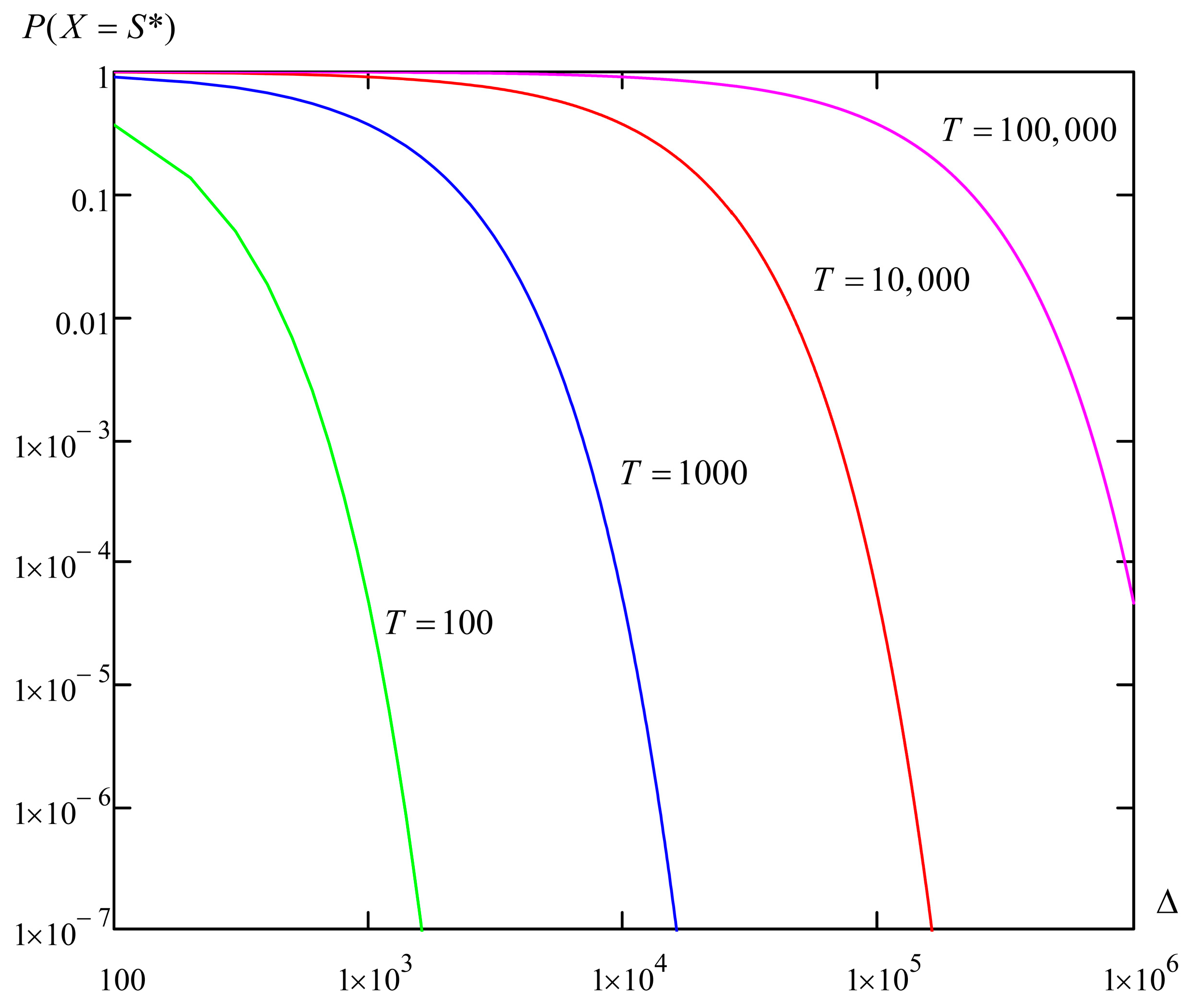
5. Results
6. Discussion of the Results
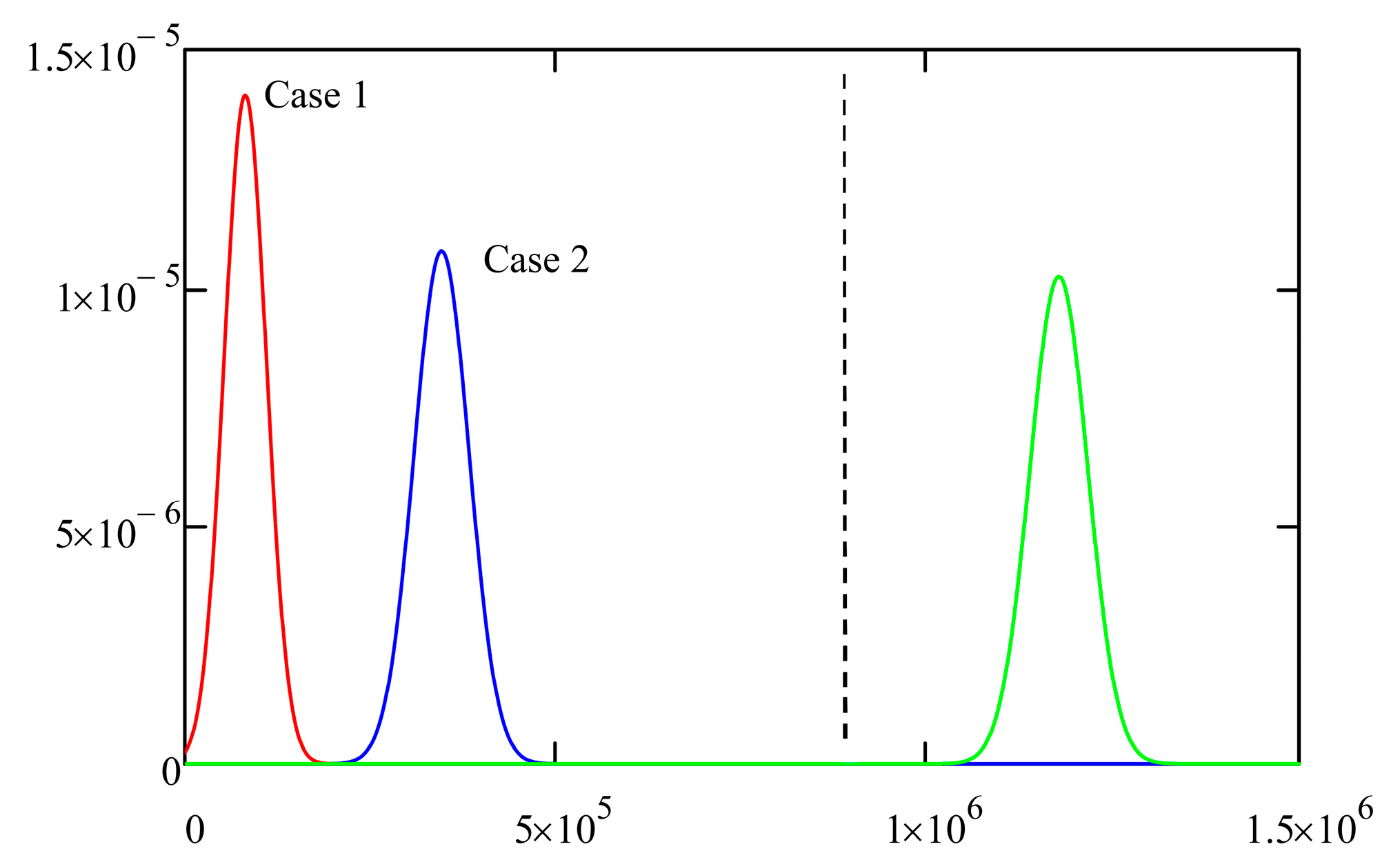
- Case 1: T0 = 100,000, α = 0.9, kout = 1000, kint = 100 (the mean is 81,359.10; the standard deviation is 28,406.44); and
- Case 2: T0 = 100,000, α = 0.7, kout = 10, kint = 10,000 (the mean is 345,715.50; the standard deviation is 37,060.07).
7. Conclusions
Author Contributions
Funding
Institutional Review Board Statement
Informed Consent Statement
Data Availability Statement
Conflicts of Interest
Appendix A
- Starting simulated annealing…
- Parameters:
- Thread count: 8
- Max outer loops in thread: 10
- Max inner loops in thread: 10,000
- Initial temperature: 1000
- Alpha parameter: 0.9
- Max frozen loops: 1,000,000
- cost = 1.56004 × 10⁸ NL = 92 temperature = 1000 Iteration = 2
- cost = 1.47575 × 10⁸ NL = 92 temperature = 1000 Iteration = 4
- …
- cost = 1.27631 × 10⁷ NL = 100 temperature = 1000 Iteration = 218
- cost = 1.25747 × 10⁷ NL = 98 temperature = 1000 Iteration = 232
- cost = 1.38404 × 10⁷ NL = 100 temperature = 1000 Iteration = 233
- cost = 1.36724 × 10⁷ NL = 98 temperature = 1000 Iteration = 235
- cost = 1.36888 × 10⁷ NL = 100 temperature = 1000 Iteration = 236
- cost = 1.32383 × 10⁷ NL = 98 temperature = 1000 Iteration = 239
- cost = 1.38281 × 10⁷ NL = 100 temperature = 1000 Iteration = 243
- cost = 1.37953 × 10⁷ NL = 100 temperature = 1000 Iteration = 245
- cost = 1.23986 × 10⁷ NL = 98 temperature = 1000 Iteration = 249
- cost = 1.21815 × 10⁷ NL = 98 temperature = 1000 Iteration = 260
- cost = 1.19685 × 10⁷ NL = 98 temperature = 1000 Iteration = 271
- cost = 1.24805 × 10⁷ NL = 100 temperature = 1000 Iteration = 280
- cost = 1.23986 × 10⁷ NL = 100 temperature = 1000 Iteration = 291
- …
- cost = 2.72794 × 10⁶ NL = 102 temperature = 1000 Iteration = 54,480
- cost = 2.69926 × 10⁶ NL = 102 temperature = 1000 Iteration = 54,801
- cost = 2.62144 × 10⁶ NL = 102 temperature = 1000 Iteration = 78,822
- cost = 2.62144 × 10⁶ NL = 102 temperature = 900 Iteration = 86,252
- SEARCH COST: 86,253
- target sbox:
- D3, 8E, E7, 8A, 12, AD, 72, 26, 81, 70, 36, 9D, 19, 37, EE, CF, FD, 38, 6D, 1C, F6, 5D, 93, BD, 68, EB, 5C, 77, 2F, 96, 01, 2C, A4, 41, 73, 07, 40, 71, F0, 2B, C1, 4B, 28, E3, AA, D9, 4C, 53, 0E, BE, B3, 1D, 43, 3E, E8, DF, E4, 9B, BB, 2E, 0A, 57, 85, 7A, 1A, E1, 47, 56, C0, ED, B1, F2, DA, AE, E0, 7D, 98, D5, 0F, AC, 25, DD, 67, 33, DC, 65, 0D, D6, DE, A6, F5, 4A, 8F, 2A, 6F, EF, 86, B9, 6E, 6C, C6, 42, 89, 39, F1, 88, A0, A8, 13, EC, 95, A7, C8, 7E, 27, A5, 7B, BA, F8, 22, 3B, 05, 90, 21, AB, 1B, 3A, F7, A9, 60, 50, 10, 18, FA, CC, 04, 5F, 8C, 78, 5A, E2, 94, 0C, 59, 9A, BF, D2, 08, 35, 46, 99, E5, 30, 82, F9, 92, 6A, 1E, 63, 49, E9, 2D, CB, DB, 7F, D8, 4E, F4, 87, 74, C9, 34, 97, 15, F3, 09, 52, 79, 7C, 45, 3C, C5, 03, 44, 58, 31, B4, 8D, 64, 8B, 3D, 3F, EA, E6, D7, D1, 54, 4D, 84, 5E, 69, 0B, 02, 20, 9E, 06, FC, A2, CE, 83, 80, AF, CD, A3, 62, 61, A1, 11, 4F, B6, 17, 5B, C7, 16, C4, BC, C3, B7, 55, 51, 29, 48, B8, 1F, 00, 6B, 24, 32, B0, 75, 9F, D4, C2, B2, 91, CA, FB, 23, B5, 76, 66, 9C, D0, FF, 14, FE,
- NL = 104
- DU = 10
- AI = 3
Appendix B
- Starting simulated annealing…
- Parameters:
- Thread count: 8
- Max outer loops in thread: 100
- Max inner loops in thread: 1000
- Initial temperature: 10,000
- Alpha parameter: 0.5
- Max frozen loops: 1,000,000
- target NL: 104
- cost = 1.19575 × 10⁸ NL = 92 temperature = 10,000 Iteration = 8
- cost = 7.38345 × 10⁷ NL = 94 temperature = 10,000 Iteration = 9
- …
- cost = 2.78036 × 10⁷ NL = 96 temperature = 10,000 Iteration = 95
- cost = 2.78077 × 10⁷ NL = 96 temperature = 10,000 Iteration = 97
- cost = 2.33759 × 10⁷ NL = 98 temperature = 10,000 Iteration = 99
- …
- cost = 2.95322 × 10⁶ NL = 102 temperature = 312.5 Iteration = 41,633
- cost = 2.95322 × 10⁶ NL = 102 temperature = 312.5 Iteration = 43,285
- …
- cost = 2.39206 × 10⁶ NL = 102 temperature = 0.0762939 Iteration = 143,542
- cost = 2.39206 × 10⁶ NL = 102 temperature = 0.038147 Iteration = 144,064
- SEARCH COST: 144,064
- target sbox:
- 31, 7D, B3, 1A, 69, 28, D3, 86, 79, 14, FB, CC, 38, 25, 5C, 3E, C7, DD, 00, 5A, 5D, 97, A7, 62, F7, D9, 60, 44, AB, AC, B6, EC, 3B, DF, 2D, 89, CD, 59, 7E, 13, B9, 78, 2E, BB, EE, A6, 7F, 85, B8, 40, D0, 4F, 30, 9C, 70, 7A, 77, 21, 32, CA, E7, E1, 15, 7B, A1, FA, BA, DA, F4, 3D, 66, 9D, 76, 3C, 84, EB, 54, E8, 26, 96, 68, 63, A4, B1, 53, 6F, 29, 8C, E5, 5F, BD, AA, 6C, A2, F0, 51, 95, 35, FE, 05, EA, F3, 7C, FF, 3A, 10, E4, 0C, 49, 99, E2, B2, E6, 34, 4C, CF, 2A, 45, 87, 50, 57, D8, D7, 91, 8F, 9F, A0, 08, 9B, EF, 16, 0E, F9, 23, 33, FC, 19, 5B, C6, F6, 93, 5E, 1E, E0, 67, 20, 1D, 6E, 24, 2C, 0F, DE, 39, BF, F1, 1B, 07, 4A, C1, B0, D4, 6D, D2, 1F, 22, FD, C4, 04, AD, B5, 72, D1, 88, 56, 92, BC, 9A, C9, 01, A8, 0A, 2B, 46, 55, ED, C5, 61, 75, 2F, 90, F8, 82, 71, 74, 11, 83, 1C, A3, 43, DB, 06, 8D, 47, 81, 12, 52, AF, 02, 4D, E3, C2, 09, 0B, B7, B4, 17, 6A, C0, AE, A9, C3, C8, 48, 80, 4B, F5, F2, 8A, 8E, 37, E9, CB, 3F, 27, 65, 6B, 9E, CE, 18, 0D, BE, 36, 64, 94, DC, 8B, A5, 73, 58, 98, D6, 41, 03, D5, 4E, 42,
- NL = 104
- DU = 10
- AI = 3
Appendix C
- Starting simulated annealing…
- Parameters:
- Thread count: 8
- Max outer loops in thread: 10,000
- Max inner loops in thread: 100
- Initial temperature: 100,000
- Alpha parameter: 0.1
- Max frozen loops: 1,000,000
- cost = 5.88431 × 10⁷ NL = 96 temperature = 100,000 Iteration = 8
- cost = 5.34364 × 10⁷ NL = 96 temperature = 100,000 Iteration = 11
- …
- cost = 1.17514 × 10⁷ NL = 98 temperature = 100,000 Iteration = 262
- cost = 1.15671 × 10⁷ NL = 98 temperature = 100,000 Iteration = 269
- cost = 1.21405 × 10⁷ NL = 100 temperature = 100,000 Iteration = 277
- cost = 1.24641 × 10⁷ NL = 98 temperature = 100,000 Iteration = 280
- cost = 1.13951 × 10⁷ NL = 98 temperature = 100,000 Iteration = 282
- cost = 1.13746 × 10⁷ NL = 98 temperature = 100,000 Iteration = 283
- cost = 1.30744 × 10⁷ NL = 100 temperature = 100,000 Iteration = 285
- cost = 1.23781 × 10⁷ NL = 100 temperature = 100,000 Iteration = 286
- cost = 1.10838 × 10⁷ NL = 98 temperature = 100,000 Iteration = 289
- cost = 1.1776 × 10⁷ NL = 100 temperature = 100,000 Iteration = 292
- cost = 1.07602 × 10⁷ NL = 100 temperature = 100,000 Iteration = 296
- cost = 1.08585 × 10⁷ NL = 100 temperature = 100,000 Iteration = 298
- cost = 1.05759 × 10⁷ NL = 100 temperature = 100,000 Iteration = 334
- cost = 1.08298 × 10⁷ NL = 100 temperature = 100,000 Iteration = 349
- cost = 1.06168 × 10⁷ NL = 100 temperature = 100,000 Iteration = 355
- cost = 1.05513 × 10⁷ NL = 100 temperature = 100,000 Iteration = 367
- cost = 1.05718 × 10⁷ NL = 100 temperature = 100,000 Iteration = 368
- cost = 1.0412 × 10⁷ NL = 100 temperature = 100,000 Iteration = 370
- …
- cost = 6.95501 × 10⁶ NL = 100 temperature = 10,000 Iteration = 759
- cost = 6.97958 × 10⁶ NL = 100 temperature = 10,000 Iteration = 797
- cost = 6.92634 × 10⁶ NL = 100 temperature = 10,000 Iteration = 800
- …
- cost = 2.60096 × 10⁶ NL = 102 temperature = 1 × 10−93 Iteration = 57,822
- cost = 2.60096 × 10⁶ NL = 102 temperature = 1 × 10−93 Iteration = 58,090
- SEARCH COST: 58,090
- target sbox:
- E1, 10, 76, 86, 92, 96, A9, 57, 7B, D9, 87, 91, 3D, C7, 06, 7D, DE, 49, 55, 80, F0, 25, 9E, 6B, 93, 64, BD, C1, 47, B4, 4D, 56, 07, 2F, 84, 23, B9, 21, B0, DC, 2D, 04, 0B, AA, 24, B5, 37, CF, 52, B6, 17, 34, 70, 08, AD, 48, D6, D5, CE, 09, 5C, F3, 0E, D2, D8, F8, 5B, B3, ED, EE, A8, B1, 5F, 95, 9D, 77, 00, BE, E4, 18, 61, DF, F1, CC, 9F, 5E, 6D, 2A, 20, 53, 7A, E2, 05, 1B, 42, 75, 3B, 4A, DD, 99, 7C, 2C, 46, 4F, FF, 35, 38, 8E, CA, D7, 7F, AE, 33, 58, 90, E0, FC, 2B, 3A, 67, 22, 02, 81, BB, 29, 1C, F5, 5D, D4, 36, CB, AC, DB, 45, C6, 2E, 14, 63, 1D, 9C, E8, B7, 94, EB, 54, F4, 8D, 01, 89, 31, FB, C8, 39, EC, AF, 69, E6, A6, A4, 43, 1E, 65, F2, 4E, 28, 8A, C9, F9, E7, 3C, 51, EA, E5, 3F, 82, 5A, FE, F6, 97, F7, 68, 30, C5, 16, BA, C3, 26, A2, DA, 6F, A3, C4, 4C, BC, 40, 72, 11, 8B, 74, 1A, B2, AB, 0D, C0, 03, 3E, 19, A7, A0, 78, 12, EF, 4B, 85, 66, 27, 0F, 62, 8F, D3, FD, C2, 8C, D0, 79, 98, 0C, 1F, 50, 60, 9A, E9, 15, 9B, 41, 6C, 88, 0A, 73, A1, 6A, 32, 59, 6E, 71, E3, 83, FA, A5, BF, B8, 13, 7E, D1, CD, 44,
- NL = 104
- DU = 10
- AI = 3
References
- Menezes, A.J.; van Oorschot, P.C.; Vanstone, S.A.; van Oorschot, P.C.; Vanstone, S.A. Handbook of Applied Cryptography; CRC Press: Boca Raton, FL, USA, 2018; ISBN 978-0-429-46633-5. [Google Scholar]
- Schneier, B. Applied Cryptography: Protocols, Algorithms, and Source Code in C; Wiley: New York, NY, USA, 1996; ISBN 978-0-471-12845-8. [Google Scholar]
- Kuznetsov, A.A.; Potii, O.V.; Poluyanenko, N.A.; Gorbenko, Y.I.; Kryvinska, N. Stream Ciphers in Modern Real-Time IT Systems; Studies in Systems, Decision and Control; Springer Nature: Cham, Switzerland, 2022; ISBN 978-3-030-79770-6. [Google Scholar]
- Carlet, C.; Ding, C. Nonlinearities of S-Boxes. Finite Fields Appl. 2007, 13, 121–135. [Google Scholar] [CrossRef]
- Carlet, C. Vectorial Boolean Functions for Cryptography. In Boolean Models and Methods in Mathematics, Computer Science, and Engineering; Cambrige University Press: New York, NY, USA, 2006. [Google Scholar]
- Matsui, M. Linear Cryptanalysis Method for DES Cipher. In Advances in Cryptology, Proceedings of the EUROCRYPT ’93: Workshop on the Theory and Application of Cryptographic Techniques Lofthus, Norway, 23–27 May 1993; Helleseth, T., Ed.; Springer: Berlin/Heidelberg, Germany, 1994; pp. 386–397. [Google Scholar]
- Mihailescu, M.I.; Nita, S.L. Linear and Differential Cryptanalysis. In Pro Cryptography and Cryptanalysis: Creating Advanced Algorithms with C# and .NET; Mihailescu, M.I., Nita, S.L., Eds.; Apress: Berkeley, CA, USA, 2021; pp. 457–481. ISBN 978-1-4842-6367-9. [Google Scholar]
- Biham, E.; Perle, S. Conditional Linear Cryptanalysis—Cryptanalysis of DES with Less Than 242 Complexity. IACR Trans. Symmetric Cryptol. 2018, 3, 215–264. [Google Scholar] [CrossRef]
- Freyre Echevarría, A. Evolución Híbrida de S-Cajas No Lineales Resistentes a Ataques de Potencia. Master’s Thesis, Universidad de La Habana, Havana, Cuba, 2020. [Google Scholar]
- Álvarez-Cubero, J. Vector Boolean Functions: Applications in Symmetric Cryptography. Ph.D. Thesis, Universidad Politécnica de Madrid, Madrid, Spain, 2015. [Google Scholar]
- Picek, S.; Cupic, M.; Rotim, L. A New Cost Function for Evolution of S-Boxes. Evol. Comput. 2016, 24, 695–718. [Google Scholar] [CrossRef] [PubMed]
- Freyre-Echevarría, A.; Martínez-Díaz, I.; Pérez, C.M.L.; Sosa-Gómez, G.; Rojas, O. Evolving Nonlinear S-Boxes with Improved Theoretical Resilience to Power Attacks. IEEE Access 2020, 8, 202728–202737. [Google Scholar] [CrossRef]
- Ars, G.; Faugère, J.-C. Algebraic Immunities of Functions over Finite Fields; INRIA: Paris, France, 2005; p. 17. [Google Scholar]
- Courtois, N.T.; Bard, G.V. Algebraic Cryptanalysis of the Data Encryption Standard. In Cryptography and Coding, Proceedings of the 11th IMA International Conference, Cirencester, UK, 18–20 December 2007; Galbraith, S.D., Ed.; Springer: Berlin/Heidelberg, Germany, 2007; pp. 152–169. [Google Scholar]
- Bard, G.V. Algebraic Cryptanalysis; Springer: Boston, MA, USA, 2009; ISBN 978-0-387-88756-2. [Google Scholar]
- Daemen, J.; Rijmen, V. Specification of Rijndael. In The Design of Rijndael: The Advanced Encryption Standard (AES); Daemen, J., Rijmen, V., Eds.; Information Security and Cryptography; Springer: Berlin/Heidelberg, Germany, 2020; pp. 31–51. ISBN 978-3-662-60769-5. [Google Scholar]
- Courtois, N.T.; Pieprzyk, J. Cryptanalysis of Block Ciphers with Overdefined Systems of Equations. In Advances in Cryptology, Proceedings of the ASIACRYPT 2002: 8th International Conference on the Theory and Application of Cryptology and Information Security Queenstown, New Zealand, 1–5 December 2002; Zheng, Y., Ed.; Springer: Berlin/Heidelberg, Germany, 2002; pp. 267–287. [Google Scholar]
- Gorbenko, I.; Kuznetsov, A.; Gorbenko, Y.; Pushkar’ov, A.; Kotukh, Y.; Kuznetsova, K. Random S-Boxes Generation Methods for Symmetric Cryptography. In Proceedings of the 2019 IEEE 2nd Ukraine Conference on Electrical and Computer Engineering (UKRCON), Lviv, Ukraine, 2–6 July 2019; pp. 947–950. [Google Scholar]
- Clark, A.J. Optimisation Heuristics for Cryptology. Ph.D. Thesis, Queensland University of Technology, Brisbane City, Australia, 1998. [Google Scholar]
- Millan, W. How to Improve the Nonlinearity of Bijective S-Boxes. In Information Security and Privacy, Proceedings of the Third Australasian Conference, ACISP’98, Brisbane, Australia, 13–15 July 1998; Boyd, C., Dawson, E., Eds.; Springer: Berlin/Heidelberg, Germany, 1998; pp. 181–192. [Google Scholar]
- Clark, J.A.; Jacob, J.L.; Stepney, S. The Design of S-Boxes by Simulated Annealing. In Proceedings of the 2004 Congress on Evolutionary Computation (IEEE Cat. No.04TH8753), Portland, OR, USA, 19–23 June 2004; Volume 2, pp. 1533–1537. [Google Scholar]
- Burnett, L.D. Heuristic Optimization of Boolean Functions and Substitution Boxes for Cryptography. Ph.D. Thesis, Queensland University of Technology, Brisbane City, Australia, 2005. [Google Scholar]
- Delahaye, D.; Chaimatanan, S.; Mongeau, M. Simulated Annealing: From Basics to Applications. In Handbook of Metaheuristics; [Gendreau, M., Potvin, J.-Y., Eds.; International Series in Operations Research & Management Science; Springer International Publishing: Cham, Switzerland, 2019; Volume 272, pp. 1–35. ISBN 978-3-319-91085-7. [Google Scholar]
- McLaughlin, J.; Clark, J.A. Using Evolutionary Computation to Create Vectorial Boolean Functions with Low Differential Uniformity and High Nonlinearity. arXiv 2013, arXiv:1301.6972. [Google Scholar]
- Kuznetsov, A.; Wieclaw, L.; Poluyanenko, N.; Hamera, L.; Kandiy, S.; Lohachova, Y. Optimization of a Simulated Annealing Algorithm for S-Boxes Generating. Sensors 2022, 22, 6073. [Google Scholar] [CrossRef] [PubMed]
- Freyre Echevarría, A.; Martínez Díaz, I. A New Cost Function to Improve Nonlinearity of Bijective S-Boxes. Symmetry 2020, 12, 1896. [Google Scholar] [CrossRef]
- Kuznetsov, A.; Poluyanenko, N.; Kandii, S.; Zaichenko, Y.; Prokopovich-Tkachenko, D.; Katkova, T. Optimizing the Local Search Algorithm for Generating S-Boxes. In Proceedings of the 2021 IEEE 8th International Conference on Problems of Infocommunications, Science and Technology (PIC S T), Kharkiv, Ukraine, 5–7 October 2021; pp. 458–464. [Google Scholar]
- Freyre-Echevarría, A.; Alanezi, A.; Martínez-Díaz, I.; Ahmad, M.; Abd El-Latif, A.A.; Kolivand, H.; Razaq, A. An External Parameter Independent Novel Cost Function for Evolving Bijective Substitution-Boxes. Symmetry 2020, 12, 1896. [Google Scholar] [CrossRef]
- Millan, W.; Clark, A.; Dawson, E. Boolean Function Design Using Hill Climbing Methods. In Information Security and Privacy, Proceedings of the 4th Australasian Conference, ACISP’99 Wollongong, NSW, Australia, 7–9 April 1999; Pieprzyk, J., Safavi-Naini, R., Seberry, J., Eds.; Springer: Berlin/Heidelberg, Germany, 1999; pp. 1–11. [Google Scholar]
- Millan, W.; Clark, A. Smart Hill Climbing Finds Better Boolean Functions. In Workshop on Selected Areas in Cryptology; Queensland University of Technology: Queensland, Australia, 1997. [Google Scholar]
- Souravlias, D.; Parsopoulos, K.E.; Meletiou, G.C. Designing Bijective S-Boxes Using Algorithm Portfolios with Limited Time Budgets. Appl. Soft Comput. 2017, 59, 475–486. [Google Scholar] [CrossRef]
- Wang, J.; Zhu, Y.; Zhou, C.; Qi, Z. Construction Method and Performance Analysis of Chaotic S-Box Based on a Memorable Simulated Annealing Algorithm. Symmetry 2020, 12, 2115. [Google Scholar] [CrossRef]
- Friedli, S.; Velenik, Y. Statistical Mechanics of Lattice Systems: A Concrete Mathematical Introduction, 1st ed.; Cambridge University Press: Cambridge, UK, 2017; ISBN 978-1-107-18482-4. [Google Scholar]
- Eremia, M.; Liu, C.-C.; Edris, A.-A. Heuristic Optimization Techniques. In Advanced Solutions in Power Systems: HVDC, FACTS, and Artificial Intelligence; IEEE: Manhattan, NY, USA, 2016; pp. 931–984. ISBN 978-1-119-17533-9. [Google Scholar]
- Laskari, E.C.; Meletiou, G.C.; Vrahatis, M.N. Utilizing Evolutionary Computation Methods for the Design of S-Boxes. In Proceedings of the 2006 International Conference on Computational Intelligence and Security, Guangzhou, China, 3–6 November 2006; Volume 2, pp. 1299–1302. [Google Scholar]
- Tesar, P. A New Method for Generating High Non-Linearity S-Boxes. Radioengineering 2010, 19, 23–26. [Google Scholar]
- Eiben, A.E.; Smith, J.E. Genetic Algorithms. In Introduction to Evolutionary Computing; Eiben, A.E., Smith, J.E., Eds.; Natural Computing Series; Springer: Berlin/Heidelberg, Germany, 2003; pp. 37–69. ISBN 978-3-662-05094-1. [Google Scholar]
- Ivanov, G.; Nikolov, N.; Nikova, S. Cryptographically Strong S-Boxes Generated by Modified Immune Algorithm. In Cryptography and Information Security in the Balkans, Proceedings of the Second International Conference, BalkanCryptSec 2015, Koper, Slovenia, 3-4 September 2015; Pasalic, E., Knudsen, L.R., Eds.; Springer International Publishing: Cham, Switzerland, 2016; pp. 31–42. [Google Scholar]


| , | , | , | |
|---|---|---|---|
| 76,009.67 (100%) | 79,524.40 (100%) | 80,626.22 (100%) | |
| 81,687.52 (100%) | 90,611.95 (100%) | 78,434.70 (100%) | |
| 81,329.86 (100%) | 88,245.98 (100%) | 85,446.05 (100%) | |
| 80,237.73 (100%) | 72,907.94 (100%) | 90,480.17 (100%) | |
| 92,201.78 (100%) | 82,822.92 (100%) | 85,577.41 (100%) | |
| 85,267.11 (100%) | 80,468.54 (100%) | 83,661.40 (100%) | |
| 86,358.69 (100%) | 79,653.47 (100%) | 83,008.08 (100%) | |
| 77,112.92 (100%) | 82,100.52 (100%) | 85,446.05 (100%) | |
| 80,084.09 (100%) | 84,360.09 (100%) | 80,019.55 (100%) |
| , | , | , | |
|---|---|---|---|
| 82,530.71 (100%) | 84,092.05 (100%) | 82,686.53 (100%) | |
| 83,479.26 (100%) | 81,281.64 (100%) | 83,755.94 (100%) | |
| 84,975.59 (100%) | 79,385.64 (100%) | 88,544.81 (100%) | |
| 82,686.68 (100%) | 83,480.77 (100%) | 93,185.31 (100%) | |
| 82,397.30 (100%) | 81,515.59 (100%) | 80,625.44 (100%) | |
| 85,553.65 (100%) | 78,870.06 (100%) | 82,309.30 (100%) | |
| 83,126.02 (100%) | 89,313.00 (100%) | 86,520.43 (100%) | |
| 78,633.10 (100%) | 82,243.44 (100%) | 81,308.54 (100%) | |
| 86,604.24 (100%) | 90,141.24 (100%) | 83,131.90 (100%) |
| , | , | , | |
|---|---|---|---|
| 81,975.30 (100%) | 79,378.70 (100%) | 83,423.39 (100%) | |
| 88,910.29 (100%) | 88,009.86 (100%) | 83,627.32 (100%) | |
| 84,952.69 (100%) | 83,338.59 (100%) | 77,009.26 (100%) | |
| 80,722.98 (100%) | 82,152.62 (100%) | 90,112.30 (100%) | |
| 75,690.74 (100%) | 83,605.75 (100%) | 84,112.64 (100%) | |
| 82,985.41 (100%) | 82,453.39 (100%) | 80,729.33 (100%) | |
| 86,407.67 (100%) | 82,462.94 (100%) | 84,714.74 (100%) | |
| 82,742.78 (100%) | 80,918.05 (100%) | 86,715.16 (100%) | |
| 81,975.30 (100%) | 79,378.70 (100%) | 83,423.39 (100%) |
| , | , | , | |
|---|---|---|---|
| 129,340.79 (100%) | 82,815.54 (100%) | 84,054.20 (100%) | |
| 153,047.44 (100%) | 88,950.34 (100%) | 80,751.58 (100%) | |
| 177,362.26 (100%) | 83,268.43 (100%) | 79,454.68 (100%) | |
| 185,580.21 (100%) | 86,333.64 (100%) | 82,799.83 (100%) | |
| 226,627.30 (100%) | 92,578.85 (100%) | 91,702.98 (100%) | |
| 281,077.52 (100%) | 87,348.77 (100%) | 80,655.30 (100%) | |
| 345,715.50 (100%) | 94,778.97 (100%) | 83,609.55 (100%) | |
| 503,914.17 (100%) | 106,267.47 (100%) | 79,737.76 (100%) | |
| - (0%) | 153,180.84 (100%) | 81,359.10 (100%) |
| Value Interval | (Normal Distribution) | (Empirical Data) | |
|---|---|---|---|
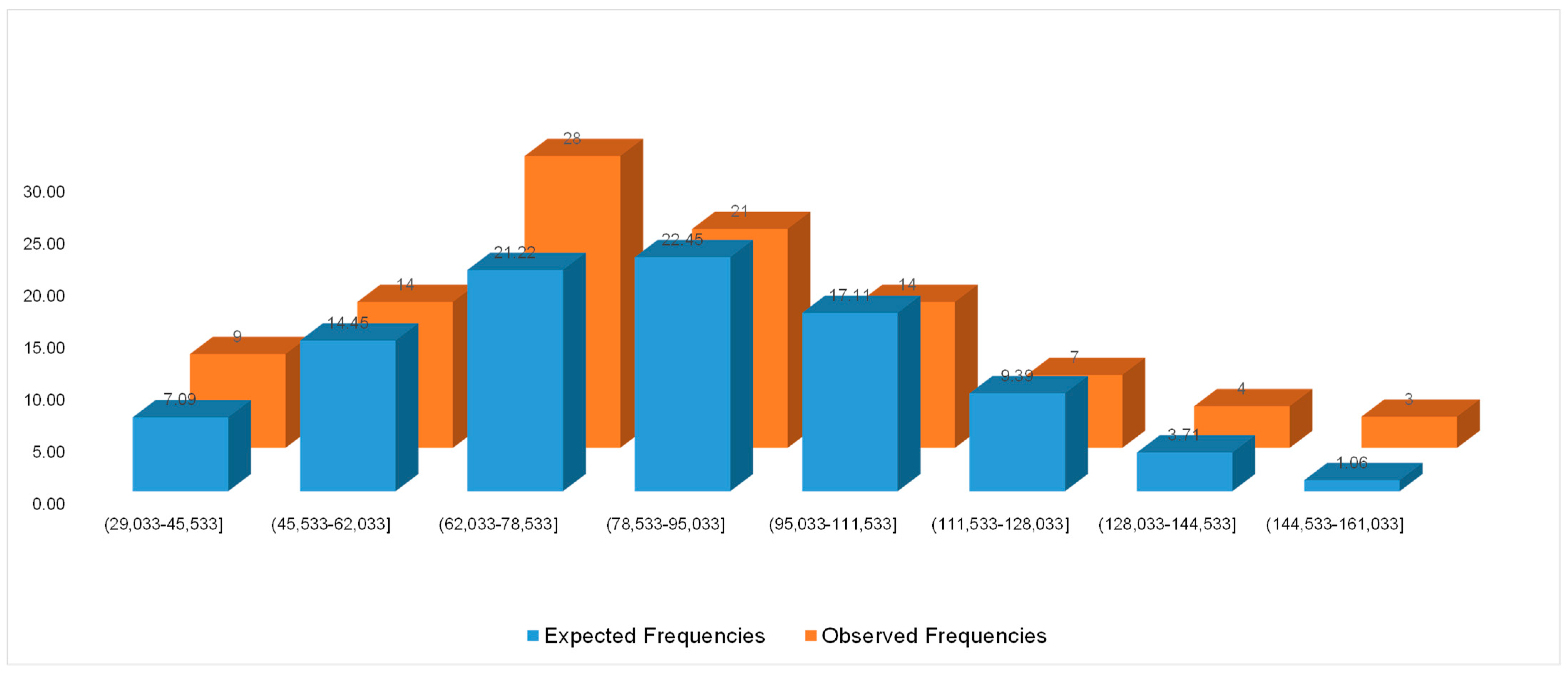
| (29,033–45,533] | 7.09 | 9 | 0.52 |
| (45,533–62,033] | 14.45 | 14 | 0.01 |
| (62,033–78,533] | 21.22 | 28 | 2.16 |
| (78,533–95,033] | 22.45 | 21 | 0.09 |
| (95,033–111,533] | 17.11 | 14 | 0.56 |
| (111,533–128,033] | 9.39 | 7 | 0.61 |
| (128,033–144,533] | 3.71 | 4 | 0.02 |
| (144,533–161,033] | 1.06 | 3 | 3.58 |
| intervals | 7.56 | ||
| . The critical region is >11.070498 | |||
| Value interval | (Normal Distribution) | (Empirical Data) | |
|---|---|---|---|
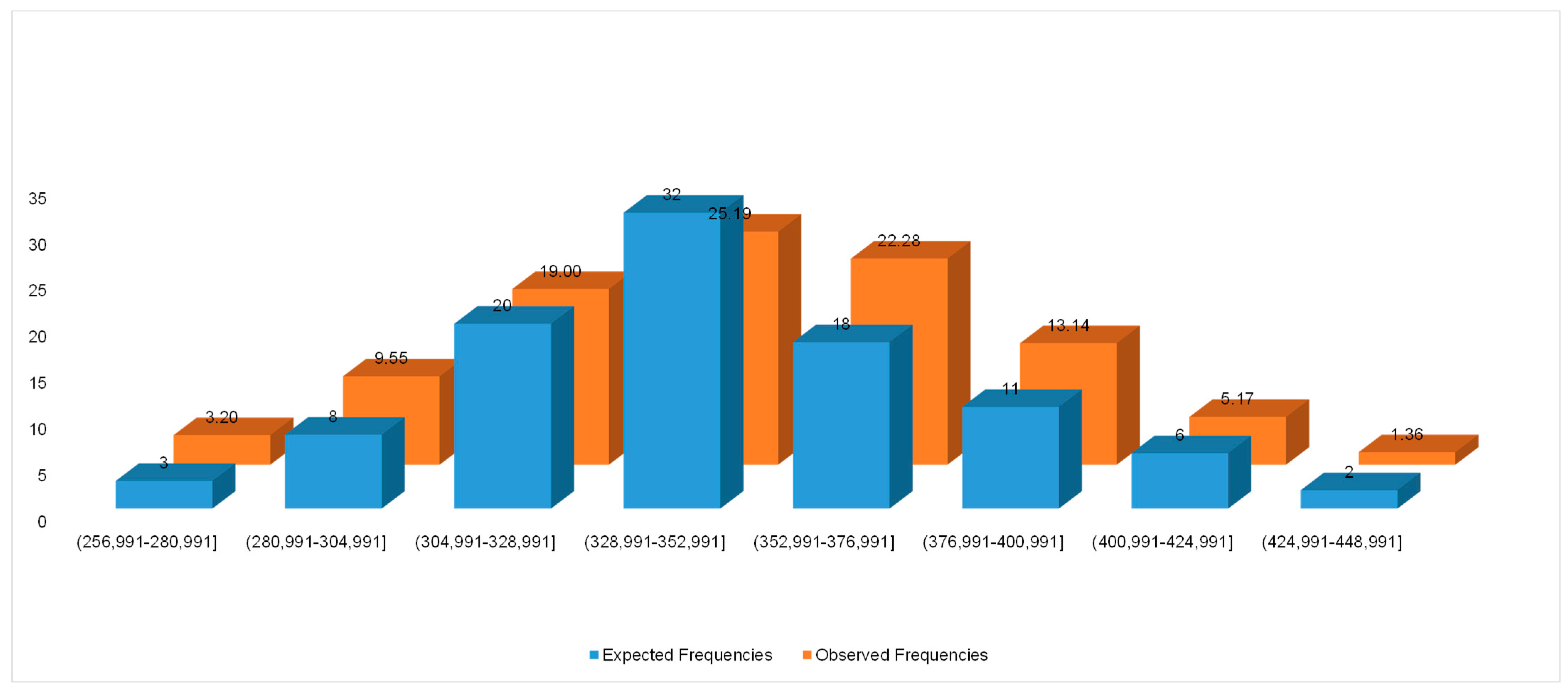
| (256,991–280,991] | 3.20 | 3 | 0.01 |
| (280,991–304,991] | 9.55 | 8 | 0.25 |
| (304,991–328,991] | 19.00 | 20 | 0.05 |
| (328,991–352,991] | 25.19 | 32 | 1.84 |
| (352,991–376,991] | 22.28 | 18 | 0.82 |
| (376,991–400,991] | 13.14 | 11 | 0.35 |
| (400,991–424,991] | 5.17 | 6 | 0.13 |
| (424,991–448,991] | 1.36 | 2 | 0.31 |
| intervals | 3.77 | ||
| . The critical region is >11.070498 | |||
Disclaimer/Publisher’s Note: The statements, opinions and data contained in all publications are solely those of the individual author(s) and contributor(s) and not of MDPI and/or the editor(s). MDPI and/or the editor(s) disclaim responsibility for any injury to people or property resulting from any ideas, methods, instructions or products referred to in the content. |
© 2023 by the authors. Licensee MDPI, Basel, Switzerland. This article is an open access article distributed under the terms and conditions of the Creative Commons Attribution (CC BY) license (https://creativecommons.org/licenses/by/4.0/).
Share and Cite
Kuznetsov, A.; Karpinski, M.; Ziubina, R.; Kandiy, S.; Frontoni, E.; Peliukh, O.; Veselska, O.; Kozak, R. Generation of Nonlinear Substitutions by Simulated Annealing Algorithm. Information 2023, 14, 259. https://doi.org/10.3390/info14050259
Kuznetsov A, Karpinski M, Ziubina R, Kandiy S, Frontoni E, Peliukh O, Veselska O, Kozak R. Generation of Nonlinear Substitutions by Simulated Annealing Algorithm. Information. 2023; 14(5):259. https://doi.org/10.3390/info14050259
Chicago/Turabian StyleKuznetsov, Alexandr, Mikolaj Karpinski, Ruslana Ziubina, Sergey Kandiy, Emanuele Frontoni, Oleksandr Peliukh, Olga Veselska, and Ruslan Kozak. 2023. "Generation of Nonlinear Substitutions by Simulated Annealing Algorithm" Information 14, no. 5: 259. https://doi.org/10.3390/info14050259