Abstract
Falls are a significant health concern leading to increased morbidity and healthcare costs, especially for the elderly. Early and accurate detection of fall events is critical for timely intervention and preventing severe complications. This study presents a novel approach to triaxial accelerometer signals by employing data-adaptive Gaussian average filtering (DAGAF) decomposition in conjunction with machine learning techniques for fall detection. The triaxial accelerometer signals from the FallAllD dataset were decomposed into intrinsic mode functions (IMFs) and a residual component, from which feature vectors were extracted to train support vector machine (SVM) and k-nearest neighbor (kNN) classifiers. Experimental results demonstrate that the combination of the first and the third IMFs with the residual component yields the highest classification accuracy of 96.34%, with SVM outperforming kNN across all performance metrics. This approach significantly improves fall detection accuracy compared to using raw accelerometer signals, highlighting its potential in enhancing wearable fall detection systems. The proposed DAGAF decomposition method not only enhances feature extraction but also provides a promising advancement in the field, suggesting its potential to increase the reliability and accuracy of fall detection in practical applications.
1. Introduction
According to the World Health Organization (WHO), a fall is defined as an unexpected event that results in a person inadvertently coming to rest on the ground, the floor, or another lower level [1]. Falls and their related injuries pose significant health risks, particularly for the elderly. These incidents adversely affect functional independence and quality of life, and are closely associated with increased morbidity, mortality, and healthcare costs [2]. With at least 28% of individuals aged 65 or older experiencing one or more falls annually [3,4], falls have become a critical public health concern. Fatal falls rank as the second leading cause of unintentional injury deaths worldwide, surpassed only by traffic injuries [1]. Early and accurate fall detection is essential for timely intervention and preventing severe complications. Numerous approaches have been explored for fall detection, as extensively reviewed in several articles [5,6,7]. In addition to wearable devices, ambient devices, and cameras [5], other technologies such as acoustics [8], WiFi [9,10], light detection and ranging (LiDAR) technology [11,12], and millimeter-wave (mmWave) radar [13] have also been utilized for fall detection. Multimodal data fusion is another promising technique that has been investigated for this purpose [14]. Given that over 80% of fall-related fatalities occur in low- and middle-income countries [1], there is a critical demand for cost-effective fall detection solutions. Advancements in microelectromechanical system (MEMS) technology have made accelerometers widely available, making wearable devices equipped with these sensors a particularly promising approach for addressing this issue [15]. Feature extraction plays a crucial role in identifying fall events from accelerometer signals, which is essential for effective fall detection. Palmerini et al. proposed a wavelet-based approach for fall detection, in which the mother wavelet was adaptively optimized based on the input accelerometer signal [16]. The main limitations of this study include a relatively high number of false alarms and the use of a small test sample size. Time-frequency analysis using the continuous wavelet transform (CWT) has also been applied to the analysis of accelerometer signal [17]. The CWT spectrogram enables the analysis of instantaneous frequency variations over time while preserving good frequency resolution. Another method that can simultaneously present both time and frequency information is the Hilbert–Huang transform (HHT) [18], which was applied by Erfianto et al. to accelerometer signal for gait analysis [19]. However, time–frequency analysis generally requires more computing resources in terms of data storage and processing speed, which becomes especially critical in scenarios involving wearable fall alarm devices. This demand is particularly pronounced with the HHT due to its reliance on empirical mode decomposition (EMD) [18] or ensemble empirical mode decomposition (EEMD) [20]. The repeated interpolation processes required to extract the intrinsic mode functions (IMFs) significantly increase the computational burden, making the implementation of such an algorithm on a microcontroller unit (MCU) for the wearable device a challenging task. In addition to feature extraction from triaxial accelerometer signals [21], incorporating machine learning [7] and deep learning [6] to improve recognition accuracy has also become a popular research direction. Moreover, Šeketa et al. employed event-centered data segmentation to evaluate detection performance in different window configurations [22]. Santoyo-Ramón et al. utilized one-class classifiers (OCCs) by training the model solely on the majority data from activities of daily living (ADLs), achieving detection performance comparable to that obtained with supervised binary classification [23]. Liu et al. proposed a deep learning-based approach for enhancing accelerometer signals which significantly improved the fall detection accuracy at low sampling rates [24]. Despite these advancements, there remains a demand for innovative techniques that can further improve the accuracy and reliability of fall detection.
This paper explores this issue from a new perspective that has not been investigated in previous studies by utilizing a signal decomposition algorithm for triaxial accelerometer signals before feature extraction. The novel data-adaptive Gaussian average filtering (DAGAF) algorithm [25] is employed to decompose triaxial accelerometer signals into IMFs and the residual component. The performance (including accuracy, sensitivity, specificity, precision, and -score) is compared across various combinations of the decomposed components and the raw triaxial accelerometer signals using machine learning-based classifiers. Performance is also evaluated using different event-based time segments. The results demonstrate that the DAGAF decomposition improves fall detection performance, offering a promising advancement in the field and providing a new direction for future research on signal processing in wearable monitoring devices.
The rest of this paper is organized as follows. Section 2 primarily contains the dataset used, the proposed DAGAF algorithm, feature extraction, classifiers, and the performance metrics. The experimental results and the related discussion are presented in Section 3. Finally, the conclusions are given in Section 4.
2. Materials and Methods
This section is divided into two parts. The first part (Section 2.1) provides details on the dataset used, along with the computing resources (including the software and computing environment) employed in this research. The second part (Section 2.2) introduces the proposed DAGAF decomposition and the associated methods used for verification.
2.1. Materials
2.1.1. Dataset
This study utilized the FallAllD dataset, which was developed by Saleh et al. [15] and can be accessed on IEEE DataPort™ [26]. To capture movement during the experiment, inertial measurement units (IMUs) were placed on the subjects’ neck, chest, and waist. Each IMU contains a triaxial accelerometer (sampling frequency: 238 Hz, measurement range: 8 g), a triaxial gyroscope (sampling frequency: 238 Hz, angular rate: 2000 dps), a triaxial magnetometer (sampling frequency: 80 Hz, full-scale magnetic field: 4 Gauss), and a barometer (sampling frequency: 10 Hz). Özdemir’s study [27] found that fall detection systems using waist-worn accelerometers perform better than those with accelerometers placed at other locations. This study thus focused exclusively on triaxial accelerometer signals collected from the waist.
This dataset was originally collected from 15 healthy young adults (8 males, 7 females) with an average age of 32 years, an average height of 171 cm, and an average weight of 67 kg. To ensure data consistency and relevance, only the data from 10 subjects who performed both fall and ADL scenarios were included in the analysis. The dataset used in this research consists of 1053 ADL instances and 423 fall trials.
Each signal in the original dataset has a duration of 20 s. A previous investigation identified that an impact-defined window consisting of 2 s before the impact (backward) and 1.23 s after the impact (forward) yielded the best performance on the FallAllD dataset [28]. Accordingly, the same impact-defined data segmentation was adopted in this study. Specifically, the peak summarized energy from triaxial accelerometer signals occurred at the 2-s mark, resulting in a length of 3.23 s for each data instance in the dataset used.
2.1.2. Computing Resources
The codes for DAGAF decomposition have been developed in both Python and MATLAB (MathWorks Inc., Natick, Massachusetts, USA), and are available on GitHub [29]. The Python implementation was created using Python 3.9.12, along with the NumPy (version 1.21.5), SciPy (version 1.7.3), and Matplotlib (version 3.5.3) libraries. The MATLAB code was developed using MATLAB 2020b. Additionally, the Statistics and Machine Learning Toolbox is required for classification analyses involving support vector machine (SVM) and -nearest neighbor (NN) classifiers. In this study, all of the statistical tests and computational experiments were conducted in the MATLAB environment on a MacBook Pro (Apple M1 Max, 64 GB of memory, Apple Inc., Cupertino, CA, USA).
2.2. Methods
2.2.1. Data-Adaptive Gaussian Average Filtering (DAGAF) Decomposition
The process of DAGAF decomposition shares similarities with the widely used empirical mode decomposition (EMD) [18] and its modified variant, ensemble empirical mode decomposition (EEMD) [20]. The primary difference is that DAGAF employs an iterative lowpass filtering process with the Gaussian window [25], instead of the sifting procedure that extracts the instantaneous mean from the interpolated local maxima and the minima [18,20]. Beyond addressing the commonly mentioned limitations associated with EMD and EEMD (such as the boundary effect, mode mixing, unnecessary redundant decomposition, and the lack of a rigorous mathematical formulation [30]), DAGAF has demonstrated its effectiveness in analyzing nonstationary biomedical signal across a wide range of scenarios [25]. This study is the first attempt to use DAGAF to decompose triaxial accelerometer signals into IMFs and a residual component to extract the subtle fluctuations that are difficult to observe in the original signals.
Let the signal to be analyzed be denoted as for . Note that may represent the accelerometer signal from the x-, y-, and z-axis, or any other signal required for further decomposition. The discrete Gaussian window with a length of points is given by
where is a parameter inversely proportional to the standard deviation of the Gaussian distribution. In this study, is set to 4.0728, resulting in the end values being as small as 0.025% of the maximum window value. Under this condition, the characteristics of the continuous-time Gaussian function are approximately preserved in its discrete-time counterpart. A notable feature is that the corresponding spectrum retains the bell shape of the Gaussian distribution centered at 0 [31]. To maintain energy consistency after filtering, a normalized Gaussian window is used in practical applications. The normalized Gaussian window is obtained as follows:
As previously mentioned, the signal is defined over the interval , while the normalized Gaussian window, as shown in Equation (2), is defined over the interval . To perform the filtering operation using , the signal must be extended at both boundaries. The developed codes provide four types of signal extension methods [29]. Following the type used in [25], this paper also employs the “double-symmetrical reflection” extension method, which has demonstrated good performance in various scenarios. This extension is applied to both boundaries in all computational experiments. The signal extended by this method is given as follows:
where denotes the mean value of . The instantaneous mean is then obtained using the moving-average operation as follows:
Due to the symmetric nature of the Gaussian window , the computation in Equation (4) is essentially a convolution sum between and . In the frequency domain, this operation corresponds to the direct multiplication between the spectra of and . Given that the spectrum of the Gaussian window forms a bell-shaped curve symmetrically centered at 0, this indicates that the moving-average operation in Equation (4) inherently functions as a lowpass filtering on by the normalized Gaussian window . The key aspect in the filtering operation is to determine the appropriate window length for . For this issue, the criterion proposed by Cicone et al. [32] is adopted in this study, and the value of is determined as follows:
where is the length of the signal to be analyzed, is the number of local extrema (including the local maxima and the local minima) present in the signal to be analyzed, is a parameter chosen around 1.6 (the value 1.6 is used in all computational experiments), and the symbol denotes the floor operation, which rounds a positive number down to the nearest integer. In the developed codes [29], the second derivative test is used to identify the locations of local extrema in the analyzed signal.
Once the instantaneous mean has been derived using Equation (4), the intrinsic mode function (IMF) can be obtained using the following expression:
Such a decomposition process is applied iteratively to using the same procedure until any predefined stop criterion is met. There are three stop criteria built in the developed codes [29]. The first one is based on the energy ratio (in dB) between the original signal and the i-th IMF, which must fall within a predefined threshold [33]. If this energy ratio exceeds the threshold, it indicates that the energy of the new IMF is significantly smaller than that of the original signal, suggesting that further decomposition is unnecessary. The second criterion assesses the energy ratio between the residual component and the separated IMF after each decomposition. If this ratio drops below a specified threshold, indicating that the residual component is nearly flat, the decomposition process will also be terminated. In the developed codes [29], the default threshold values are 20 dB for the original signal-to-IMF ratio and 0.001 for residue-to-IMF ratio, and these default values were used in all computational experiments. The third stop criterion is associated with the length of Gaussian window. Based on Equation (5), the window length is determined from the number of local extrema present in the analyzed signal. If the value of is too small, the estimated window length may exceed or be equal to the signal length. In this case, the signal to be analyzed appears to be a simple mode that is nearly flat in pattern, and it is not necessary to continue the decomposition process. Accordingly, the third stop criterion that will terminate the decomposition process is mathematically expressed as:
Given the aforementioned background, the computational procedure of DAGAF is summarized as follows:
(i) Based on the number of local extrema in the signal to be analyzed, calculate the value of using Equation (5) and verify the value of according to Equation (7). If the stop criterion is met, terminate the process. Otherwise, construct the Gaussian window of length according to Equations (1) and (2).
(ii) Extend the signal at both ends according to Equation (3) and compute the instantaneous mean using the moving-average operation as specified in Equation (4).
(iii) Derive the IMF according to Equation (6) and check if any energy ratio-based stop criterion has been fulfilled. If not, repeat steps (i) to (iii). Otherwise, terminate the entire procedure.
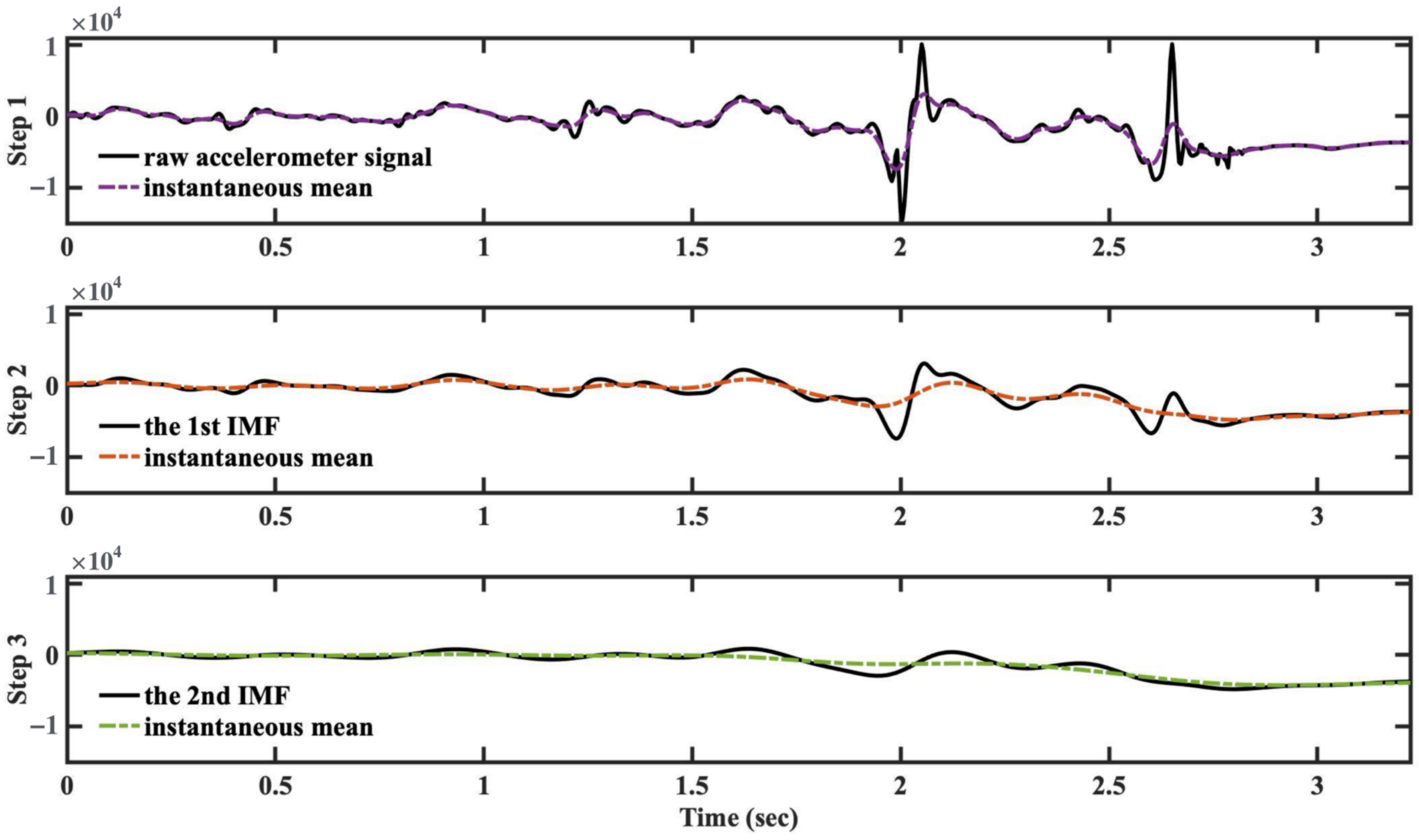
In this study, the DAGAF algorithm was employed to perform a three-level decomposition on all triaxial accelerometer signals. Specifically, each signal was processed through three iterations of decomposition, resulting in three IMFs labeled as (the first decomposed IMF), (the second decomposed IMF), and (the third decomposed IMF), respectively. The residual component, which is denoted as in this paper, represents the remaining part of the signal after extracting the three IMFs. Figure 1 presents an example of this three-level decomposition for the z-axis accelerometer signal, corresponding to a jogging to stumbling/tripping event, recorded at the waist position of subject 1 from the FallAllD dataset.
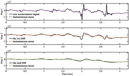
Figure 1.
Iterative procedure of three-level decomposition using the proposed DAGAF decomposition algorithm, demonstrated with the z-axis accelerometer signal (jogging to stumbling/tripping) collected at the waist position from subject 1 of the FallAllD dataset. In each subfigure, the solid line (in black color) shows the raw accelerometer signal (in Step 1) or the IMF (in Steps 2 and 3), while the dash-dotted line (in three different colors) indicates the instantaneous mean sifted by a Gaussian window.
By examining the subfigures of Figure 1 from top (Step 1) to bottom (Step 3), it can be observed that the patterns of the solid black line (representing the original raw signal in Step 1 and , in Steps 2 and 3) along with the dash-dotted line (representing the corresponding instantaneous mean at each step) become simpler and flatter progressively. This observation supports the decision to limit the decomposition process to three iterations in this study. The consistent effectiveness of this three-level decomposition across all triaxial accelerometer signals further reinforces the validity of this choice.
2.2.2. Feature Extraction
In this study, each sample consists of the accelerometer signals collected from three orthogonal axes. The raw data, without conversion to acceleration unit, were used directly in figure demonstration and computational analysis. Let and represent either the raw signals or the combination of components obtained through the DAGAF algorithm at time index n along the x-, y-, and z-axis, respectively, where . Before extracting the features, the following energy-related vectors are derived:
Having obtained , , , and , the following features are used to construct the feature vector:
(1) Statistical measures: The mean, standard deviation, and variance are computed for each of the six data, resulting in 18 features.
(2) Extreme values: The maximum, minimum, and range (the difference between the maximum and minimum) are determined for each of the six data, yielding an additional 18 features.
(3) Higher-order statistics: The skewness (the third central moment) and kurtosis (the fourth central moment) are calculated for each of the six data, adding 12 more features to the vector.
(4) Pearson’s correlation coefficients: The correlation coefficients are derived for the following pairs: versus , versus , versus , versus , versus , and versus , adding 6 more features.
In summary, a total of 54 features are included in the feature vector for each signal to be analyzed. These features have been verified to be effective in fall detection [24,34], and therefore are also adopted in this study.
2.2.3. Classifiers
To assess the effectiveness of DAGAF decomposition in fall detection, two classical machine learning classifiers, SVM and NN, were employed in this study. These classifiers have been demonstrated to be more reliable than other methods, such as naïve Bayes and decision trees, in fall detection tasks [24,34]. The classifiers used in this study are briefly described as follows:
(1) SVM is a powerful supervised learning algorithm designed to find the optimal hyperplane that separates data points from different classes with the maximum margin. The core idea of SVM is to maximize the margin between the closest data points (called support vectors) of different classes. This optimization problem can be formulated by minimizing
subject to the following constraint:
where is the weight vector that defines the hyperplane, the symbol denotes the Euclidean norm of the weight vector , is the bias term, is the feature vector of the k-th sample, is the corresponding class label for the k-th sample, and is the total number of samples. The goal of SVM is to find the weight vector and the bias that maximize the margin between classes. When the data are not linearly separable, a kernel function can be applied to map the input features into a higher-dimensional space, allowing for the separation of more complex patterns. In this study, we use the radial basis function (RBF) kernel, which is defined as:
where is a positive-valued parameter that controls the spread of the kernel, and represents the Euclidean distance between feature vectors and . The RBF kernel is particularly effective for handling nonlinear relationships in high-dimensional feature spaces. To enhance the classification performance, we used the Bayesian optimization to fine-tune the parameters of the RBF kernel, specifically the kernel parameter and the regularization parameter . The regularization term controls the trade-off between maximizing the margin and minimizing the classification error. The optimization objective function can be expressed as:
In this study, the SVM classifier was used to classify ADLs and fall activities based on the feature set consisting of 54 features (refer to Section 2.2.2 for details on feature extraction). These features capture diverse characteristics of the data, allowing the SVM classifier to detect the subtle differences between the ADL and fall classes. Both parameters and were initially set to 1.
(2) NN is an instance-based learning method used for classification. It classifies a new data point by identifying the closest neighbors in the training set and assigning the most frequent class label among these neighbors. The core concept of NN is that data points close to each other in feature space are likely to belong to the same class. Typically, proximity between data points is measured using Euclidean distance. Once the distances between the query point and all points in the training set have been obtained, the algorithm selects the nearest data points. The class label of the query point is then determined by a majority vote among these neighbors, with the most frequent class being assigned to the query point. NN is a nonparametric method, making it effective for datasets where little prior knowledge is available. Previous research [28] has shown that fall detection achieves the highest accuracy with when using Euclidean distance. Consequently, the 3NN classifier with Euclidean distance was also employed in this study. To enhance classification performance, a comprehensive set of 54 features was extracted from the proposed signal combination or the raw accelerometer signal. These features include statistical measures (mean, standard deviation, and variance), extreme values (maximum, minimum, and the range between them), higher-order statistics (skewness and kurtosis), and Pearson’s correlation coefficients. These features capture diverse characteristics of the data, enabling the NN classifier to more effectively distinguish between ADLs and fall activities with acceptable accuracy.
2.2.4. Performance Metrics
In this study, the leave-one-subject-out (LOSO) cross-validation method was employed to evaluate the classification performance. In the LOSO approach, data from a single subject are reserved as the testing dataset, while data from the remaining subjects form the training dataset. Given that the dataset used in this study consisted of 10 subjects, this process was repeated 10 times, with each subject serving as the test dataset once. The overall performance was then calculated as the average of the results across all 10 iterations.
Fall detection outcomes are classified into two categories: ADL and fall, making this a binary classification problem. In this context, a fall is considered a positive outcome, while recognizing an ADL is considered a negative outcome. The performance of a fall detection system is quantitatively assessed by categorizing the outcomes into four types of counts as follows:
(1) True positives (TP): The number of instances where the system correctly identifies a fall when the fall has actually occurred.
(2) False positives (FP): The number of instances where the system incorrectly identifies an ADL as a fall.
(3) True negatives (TN): The number of instances where the system correctly identifies an ADL when no fall has occurred.
(4) False negatives (FN): The number of instances where the system fails to identify a fall, instead incorrectly classifying it as an ADL.
The objective of a fall detection system is to minimize the occurrence of both false positives (FP) and false negatives (FN) to enhance overall performance. Common metrics for evaluating binary classification performance include accuracy, sensitivity, specificity, precision, and the -score [35]. These metrics are widely used in the literature to assess the effectiveness of fall detection systems [15,21,22,23,24,28,34]. Higher values of these metrics generally indicate better system performance.
Accuracy is defined as the ratio of correctly classified samples (both positive and negative) to the total number of samples, as given by the following equation:
Sensitivity (or recall) represents the proportion of correctly classified positive samples (i.e., falls) to the total number of actual positive samples, and is defined as follows:
Specificity (or inverse recall) is defined as the ratio of correctly classified negative samples (i.e., ADLs) to the total number of actual negative samples, and is given by
Precision represents the proportion of correctly classified positive samples to the total number of predicted positive samples, as indicated by the following equation:
-score is the harmonic mean of sensitivity and precision. It balances the trade-off between sensitivity and precision, particularly in datasets with an imbalanced class distribution. Given that the dataset used in this study comprises 1053 ADL instances and 423 fall trials, the -score offers a balanced evaluation on classification performance by accounting for both FP and FN. The -score is defined as follows:
2.2.5. Statistical Analysis
The objective of the statistical analysis was twofold. First, its aim was to examine whether there is statistical significance between the proposed signal combination and the raw accelerometer signal for each feature under the same activity (ADL or fall). Second, its objective was to determine whether the same feature shows statistical significance between ADL and fall activities within the same signal combination. Several statistical tests were employed to achieve the desired objectives. The first test was the Shapiro–Wilk normal test, which was used to assess whether the derived features of each signal combination, under the same activity, follow a normal distribution. For the first objective, a paired-samples test was conducted. If the values of the same feature are normally distributed, a paired-samples t-test was used. Otherwise, the nonparametric Wilcoxon signed-rank test was applied. For the second objective, an independent sample test was used. If the values of the same feature followed a normal distribution, an independent sample t-test was performed. Otherwise, the nonparametric Wilcoxon rank-sum test was applied.
3. Results and Discussion
In this study, the DAGAF algorithm was employed to perform a three-level decomposition on triaxial accelerometer signals. Each signal underwent this decomposition process three times, resulting in components labeled as (the first derived IMF), (the second derived IMF), (the third derived IMF), and Res (the residual component). In addition, according to the study by Liu et al. [28], the same impact-defined window, which spans 2 s before the impact (backward) and 1.23 s after the impact (forward), was adopted for the datasets in this study.
The first experiment aimed to evaluate fall detection performance by comparing the classification results obtained from various combinations of the decomposed components with those directly from the raw signals. In this experiment, fifty-four features were extracted from each signal to be analyzed (see Section 2.2.2 for details on feature extraction). Two classifiers, SVM and NN (), were employed to assess and compare their effectiveness in the fall detection task. The test results are summarized in Table 1, with the highest values highlighted in bold for each metric. The results demonstrate that combining the residual component with the raw signal or certain IMFs can enhance classification performance across both classifiers. Notably, the combinations “”, “”, and “” consistently outperformed other combinations as well as the raw signals across all tests. Specifically, the highest accuracy of 96.34% was achieved using the combination “” with the SVM classifier, which also exhibited the highest sensitivity (92.91%), specificity (98.29%), precision (95.56%), and -score (94.22%) compared to other combinations and the raw signals. Additionally, the SVM classifier consistently outperformed the NN () classifier across all metrics. For this reason, the SVM classifier was used in subsequent computational experiments. Another notable result is that the performance of the combination “” was comparable to “”. It even surpassed the latter in terms of sensitivity, precision, and -score when using the NN () classifier. Although the computation load of GADAF decomposition is relatively lighter than that of wavelet-based spectrogram and HHT, the proposed DAGAF decomposition requires an iterative filtering procedure to extract IMFs, making its implementation on an MCU for real-time applications a challenging task. However, the good performance of “” offers an alternative solution for this issue. Since is essentially a very low-frequency component contained in the raw signal, developing a lowpass filter that can adaptively extract a residual component similar to that in DAGAF decomposition seems to be a promising direction for future research.

Table 1.
Performance metrics (accuracy, sensitivity, specificity, precision, and -score) for SVM and NN classifiers across various signal combinations.
These findings suggest that incorporating the residual component along with the raw signal or the specific IMFs (the first IMF and either the second or third IMF) enhances the performance in classifying ADL and fall activities. The consistent improvement across all performance metrics highlights the effectiveness of these combinations in capturing critical information embedded in the raw signals, thereby enabling more reliable fall detection.
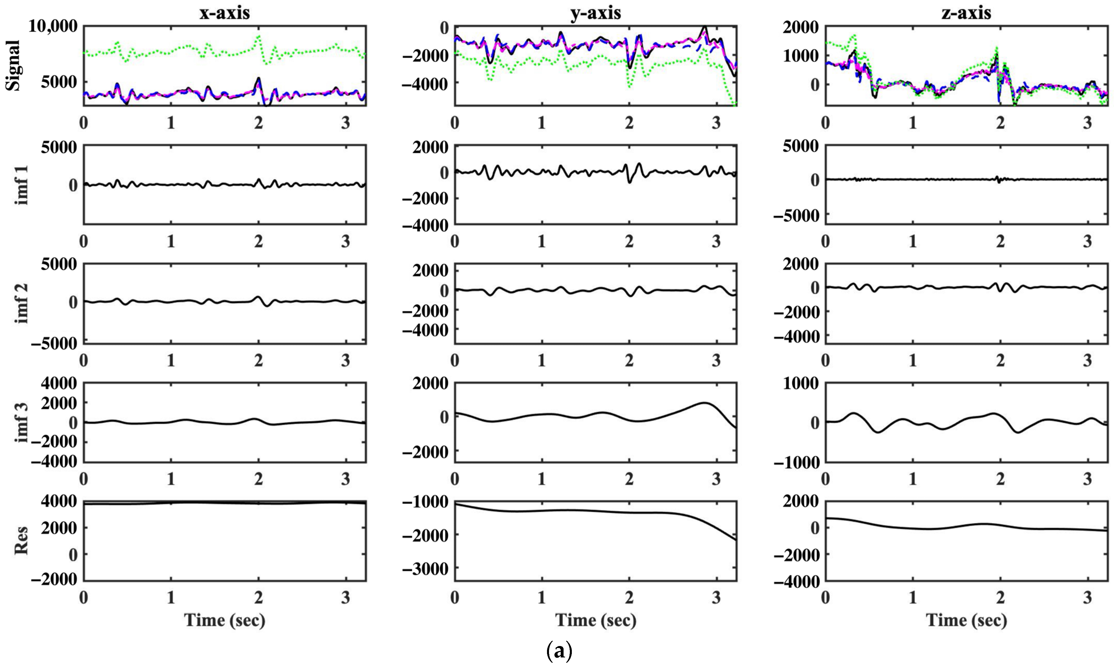
As described previously, the combinations “”, “”, and “” consistently outperform other combinations and the raw signals across all tests. By examining the patterns of the separated components after DAGAF decomposition, valuable insights can be acquired for the information captured by these decomposed components. Figure 2 presents the three-level decomposition of triaxial accelerometer signals recorded at the waist position from subject 1 of the FallAllD dataset during (a) a daily activity (sitting down) and (b) a forward fall (walking to stumbling/tripping). This decomposition reveals the IMFs and residual component for each axis, highlighting the signal characteristics associated with both ADLs and fall activities. In this figure, the vertical axis ranges were intentionally adjusted to ensure consistency at the same decomposition level for signals from both ADLs and fall activities. Notably, a marked difference was observed in , where the fall signals exhibited more densely oscillated patterns compared to the ADL signals, likely reflecting the abrupt and rapid movements appeared in a fall event. Similar distinct characteristics were also observed in , , and across all axes. Even for the low-frequency residual component (labeled as in the figure), it can be observed that the dynamic ranges during fall were greater than that during ADL activity across all axes. These differing patterns likely contribute to a more varied distribution of the extracted features in the feature space, thereby enhancing the ability of classifiers to distinguish between falls and ADLs. Moreover, as observed in Table 1, the combinations “”, “”, and “” demonstrated superior performance compared to other combinations or single decomposed components. This indicates that the richness in the oscillatory characteristics within various IMFs provides a diverse set of discriminative features, which in turn facilitates a more effective separation in the feature space when using a combination of decomposed components for the fall detection task.
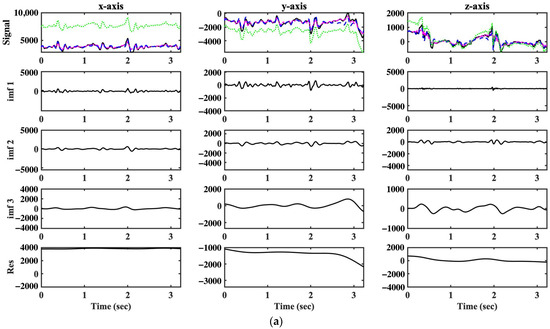
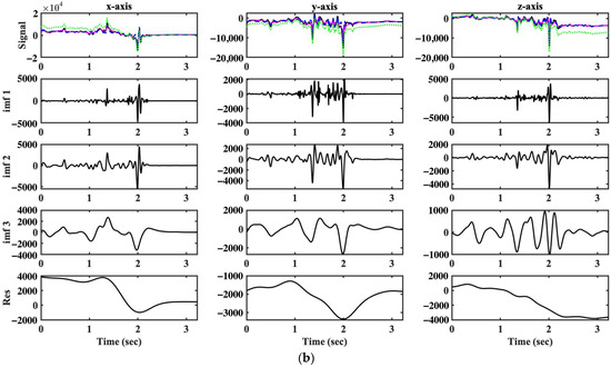
Figure 2.
Three-level decomposition of triaxial accelerometer signals collected at the waist position from subject 1 of the FallAllD dataset during (a) a daily activity (sitting down) and (b) a forward fall (walking to stumbling/tripping). In both (a,b), each subfigure (from top to bottom) presents the raw accelerometer signal (solid black line), three IMFs, and the residual component (labeled as Res) after three-level decomposition for the x-, y-, and z-axis signals (from left to right). The top subfigures in both (a,b) also display the patterns for the combinations of “” (blue dashed line), “” (green dotted line), and “” (magenta dash-dotted line).
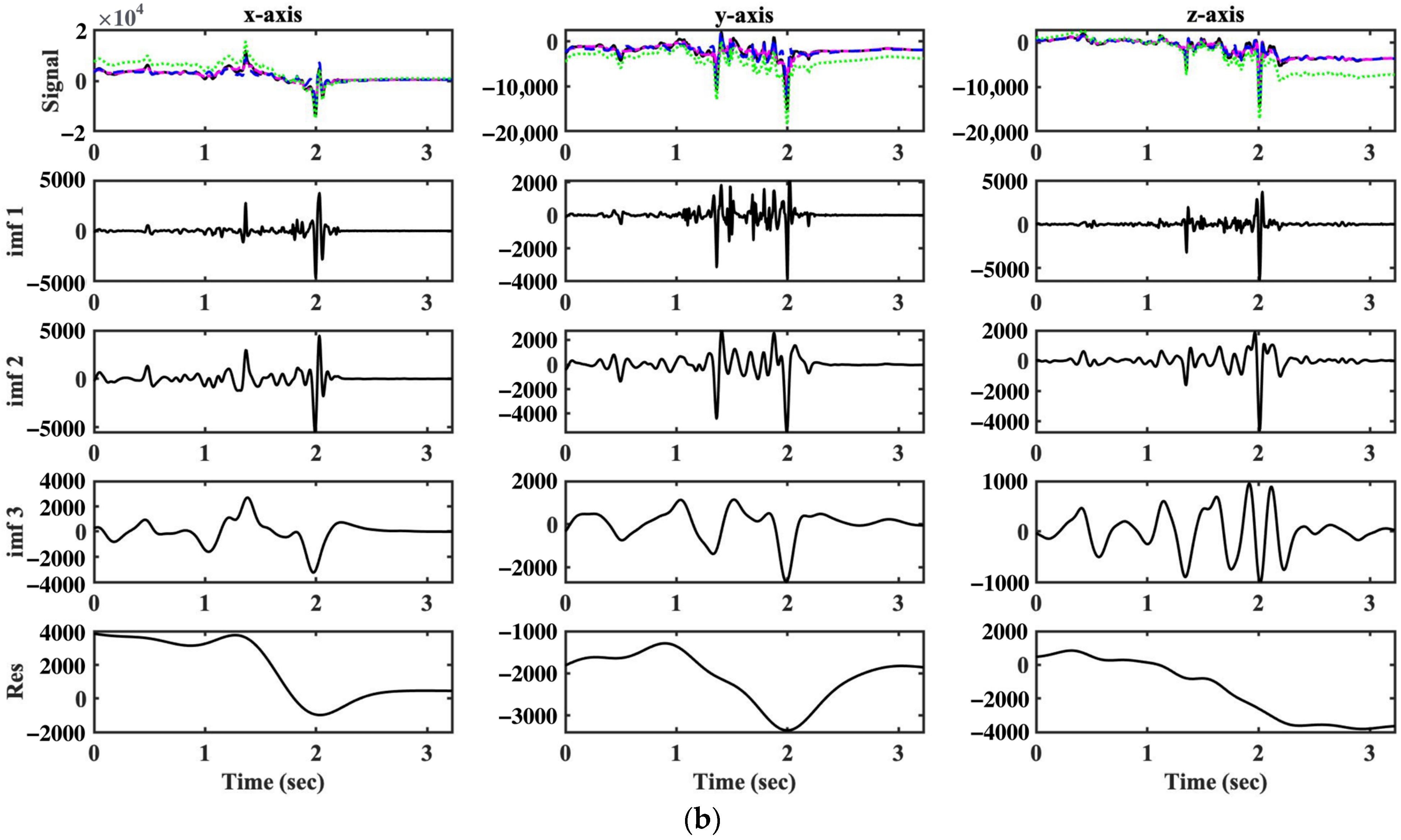
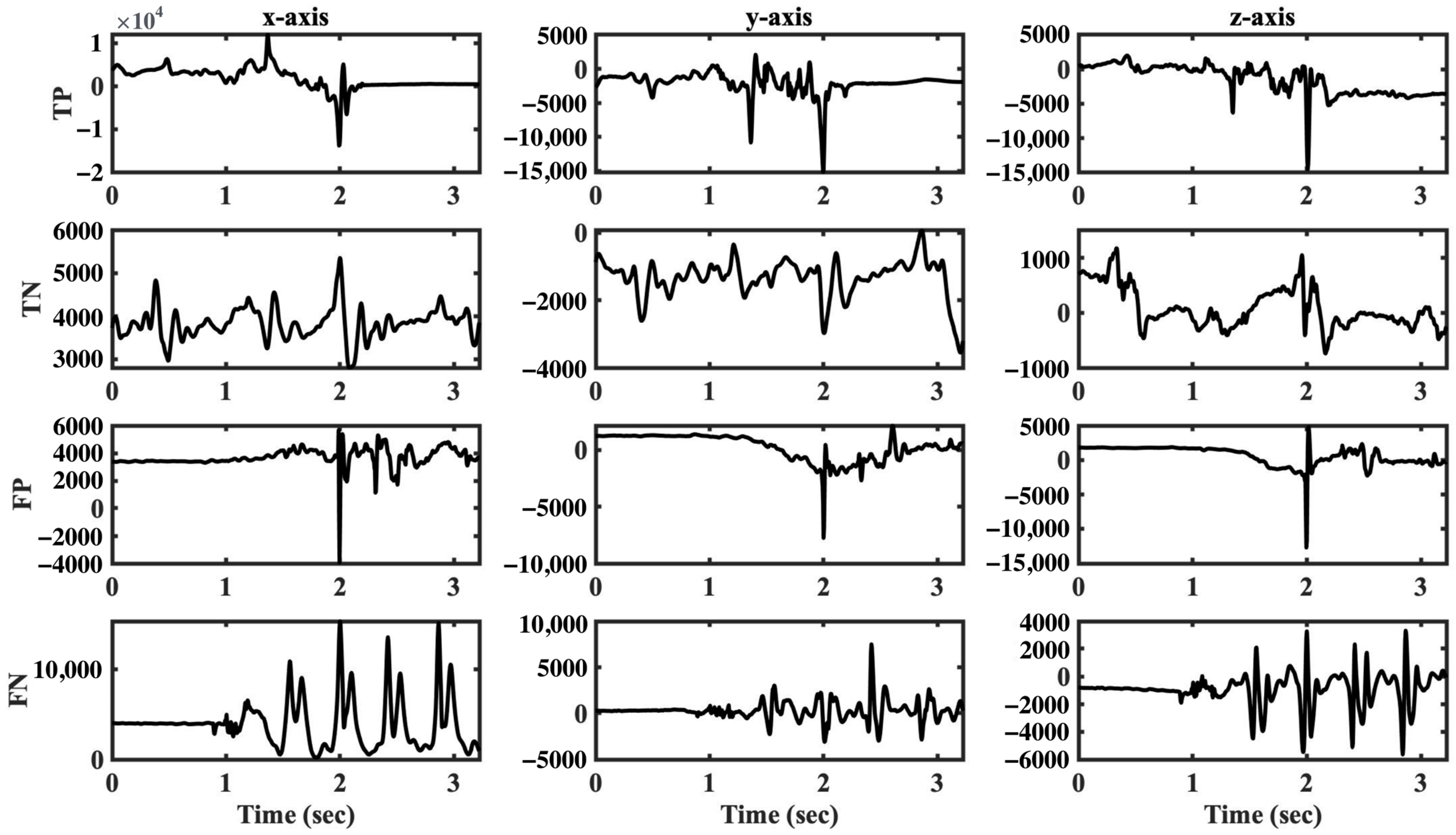
Even though a clear distinction can be observed with the help of DAGAF decomposition, analyzing the patterns of accelerometer signals in fall activities and ADLs remain a complex task. Figure 3 presents the examples of TP, TN, FP, and FN by both SVM and 3NN classifiers. The triaxial accelerometer signals shown in this figure are from subject 1 of the FallAllD dataset during a forward fall (walking to stumbling/tripping) for TP, a daily activity (sitting down) for TN, a daily activity (standing up) for FP, and from subject 2 of the FallAllD dataset during a forward fall (jogging to stumbling/tripping) for FN, respectively. From this figure, it is evident that feature engineering is necessary because the activity cannot be easily identified solely based on the patterns in the selected examples.
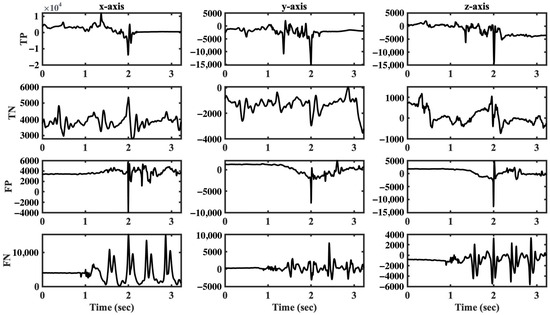
Figure 3.
Examples for TP, TN, FP, and FN (from top to bottom) by both SVM and 3NN classifiers. The triaxial accelerometer signals of the examples are from subject 1 of the FallAllD dataset during a forward fall (walking to stumbling/tripping) for TP, a daily activity (sitting down) for TN, a daily activity (standing up) for FP, and from Subject 2 of the FallAllD dataset during a forward fall (jogging to stumbling/tripping) for FN, respectively. The signals collected at the waist position are used in the examples.
To examine the characteristics of the selected features across different signal combinations in ADLs and fall activities, we also performed two types of statistical analysis. The first analysis was to verify whether there exists a statistical significance between the proposed signal combination and the raw accelerometer signal for each feature under the same activity. The second analysis was to determine whether the same feature shows a statistical significance between ADLs and fall activities within the same signal combination. The results of these tests are summarized in Table 2. The results of the Shapiro–Wilk normal test showed that none of the features in the proposed signal combinations or the raw accelerometer signals followed a normal distribution. Therefore, nonparametric methods were used for both tests. For comparing features between the proposed signal combination and the raw accelerometer signal within the same activity, the Wilcoxon signed-rank test was employed for statistical testing. The asterisk (*) in the table indicates a significant difference between the proposed signal combinations and the “raw” signal for the same feature in the same activity, evaluated at a significance level of 0.05 () using the Wilcoxon signed-rank test. For comparing features between ADL and fall activities within each signal, the Wilcoxon rank-sum test was applied. The dagger (†) in the table denotes a significant difference between ADLs and fall activities for the same feature in the same combination, evaluated at a significance level of 0.05 () using the Wilcoxon rank-sum test. The results in Table 2 indicate that the statistical significance is observed across different features, with each feature demonstrating statistical significance in at least one signal combination. This finding supports that the proposed signal combinations indeed introduce measurable statistical deviations in the feature characteristics.
Table 2.
Statistical analysis for 54 features in ADLs and fall activities across the proposed signal combinations.
Based on the study by Liu et al. [28], the same impact-defined window (2 s before the impact and 1.23 s after the impact) was adopted for the datasets in this study. In this context, the second experiment was designed to compare the performance of raw signals and three out-performing combinations (“”, “”, and “”) across five different time segments using the SVM classifier. The experimental results are summarized in Table 3, where the highest values for each metric across five different time segments are highlighted in bold. It can be observed that using signals of the whole length consistently achieves the highest performance across all metrics when compared to the signals of shorter segment. Furthermore, the combinations “”, “”, and “” generally enhanced classification performance across different time segments when compared to the raw signals. Among them, the combination “” or “” consistently achieved the best performance across all metrics and time segments. For instance, when analyzing signals of the whole segment (length of 3.23 s), the combination “” achieved an accuracy of 96.34%, sensitivity of 92.91%, specificity of 98.29%, precision of 95.56%, and an -score of 94.22%. Interestingly, the shorter segments containing the impact (which occurs at 2 s) demonstrated slightly lower yet comparable performance to the whole segment across all metrics. However, excluding the impact from the analysis segment (i.e., using the 0~1.8 s window in the experiments) results in a significant performance drop across various metrics. In this scenario, sensitivity is the most significantly impacted metric, dropping to a low value of 52.01% in the raw triaxial accelerometer signals. The low sensitivity is nearly equivalent to a random guess in classifying ADLs and fall activities. However, sensitivity increases to 68.79% while using the combination “”. This significant improvement in sensitivity underscores the advantage of using DAGAF decomposition for fall detection, even when the signal does not fully encompass the impact event. These results also suggest that including the impact event within the analysis segment is crucial for enhancing the effectiveness of fall detection.
Table 3.
Performance metrics (accuracy, sensitivity, specificity, precision, and -score) for SVM classifier applied to three different signal compositions across different time segments.
The proposed DAGAF decomposition for triaxial accelerometer signals introduces a novel approach to feature extraction in fall detection. To evaluate its effectiveness, it is essential to compare the performance of this method with that of other studies employing machine learning classifiers for fall detection. In this regard, Table 4 presents a summary of the performance metrics (accuracy, sensitivity, specificity, precision, and -score), allowing for a direct comparison between the proposed method and other studies that have used the same database (the FallAllD dataset) for fall detection. The highest values for each metric are highlighted in bold. The results in Table 4 clearly demonstrate that the proposed DAGAF method, especially the combination “”, outperforms previous studies across all metrics. Specifically, this combination achieved an accuracy of 96.34%, a sensitivity of 92.91%, a specificity of 98.29%, a precision of 95.56%, and an -score of 94.22%. These results surpass those reported in previous studies, such as Liu et al. [24], which achieved an accuracy of 95.60% and an -score of 92.16% using an enhanced preprocessing technique on triaxial accelerometer signals. The studies referenced in [15,21,22,23] did not report all performance metrics. Among these, the most competitive result is the sensitivity of 92.90% obtained by Ramón et al. [23] using the one-class NN (OC-NN) classifier trained with the majority data from ADLs, which is only slightly lower than the sensitivity achieved by the proposed approach. Please note that only the result covering the impact-window (denoted as W1) is presented in Table 4 for Šeketa et al. [22].
Table 4.
Comparison of performance metrics (accuracy, sensitivity, specificity, precision, and -score) with other studies.
In summary, the results clearly demonstrate that the proposed DAGAF decomposition consistently outperforms conventional raw signal-based approaches as well as other related studies across various performance metrics. This indicates that DAGAF decomposition significantly enhances the reliability of fall detection systems. Moreover, the superior performance of the proposed method highlights its potential for practical integration into wearable devices, where accurate and reliable fall detection is crucial.
4. Conclusions
This study presents a novel approach for fall detection by applying DAGAF decomposition to triaxial accelerometer signals in combination with machine learning classifiers. Although conceptually similar to EMD, the proposed DAGAF algorithm stands out for its unique use of Gaussian average filtering to compute the instantaneous mean. The length of Gaussian filter is dynamically adjusted based on the number of extrema in the analyzed signal, making the proposed method a data-adaptive decomposition. While the DAGAF algorithm has been successfully applied in various biomedical scenarios [25], this study marks its first application in the domain of fall detection. To facilitate further research, the detailed mathematical formulation of the DAGAF algorithm is provided, along with the codes implemented in both MATLAB and Python, which are accessible on GitHub [29].
The three-level DAGAF decomposition was consistently applied throughout all computational experiments in this study. This choice was driven by its applicability to all signals in the FallAllD dataset, thereby ensuring consistency across all analyses. After applying the three-level DAGAF decomposition, each signal was separated into components labeled as (the first derived IMF), (the second derived IMF), (the third derived IMF), and Res (the residual component). The same impact-defined window used by Liu et al. [28], which covers 2 s before the impact (backward) and 1.23 s after the impact (forward), was adopted for the dataset in this study. To evaluate the effectiveness of the proposed algorithm in fall detection, computational experiments were conducted comparing the classification performance across various component combinations against the raw signals (refer to Table 1). The results indicate that specific component combinations significantly improve classification performance in fall detection. Specifically, the combination of , , and Res with an SVM classifier achieves the highest performance metrics, with an accuracy of 96.34%, a sensitivity of 92.91%, a specificity of 98.29%, a precision of 95.56%, and an -score of 94.22%. This combination outperforms all other tested combinations, including the use of raw signals.
This study also examined the characteristics of the selected features across different signal combinations in ADLs and fall activities using two types of statistical analysis. The first analysis assessed whether there exists a statistical significance between the proposed signal combination and the raw accelerometer signal for each feature within the same activity. The second analysis evaluated whether the same feature exhibits a statistical significance between ADLs and fall activities within the same signal combination. Nonparametric methods were used in both statistical tests since none of the features in the proposed signal combinations or the raw accelerometer signals followed a normal distribution. The Wilcoxon signed-rank test was used to compare features between the proposed signal combination and the raw accelerometer signal within the same activity, while the Wilcoxon rank-sum test was employed to compare features between ADLs and fall activities within each signal. The results of these tests are summarized in Table 2. The table shows that statistical significance was observed across different features, with each feature demonstrating statistical significance in at least one signal combination. This finding indicates that the proposed signal combinations introduce statistical deviations in the feature characteristics.
To assess the impact of selected time segments on fall detection, computational experiments were conducted across five different time segments using the SVM classifier. The performance of the two top-performing combinations (“”, “”, and “”) were compared against the raw signals in classifying ADLs and fall activities (see Table 3). It was found that the combination “” or “” consistently outperformed in all performance metrics across all time segments. The signals of the whole segment (length of 3.23 s) consistently achieved higher performance metrics than those of the shorter segment. Moreover, the performance dropped significantly if the impact event was not included in the signal segment to be analyzed (0~1.8 s window in the experiments); the sensitivity dropped to 52.01% using the raw signals. However, the sensitivity increased to 68.79% for the combination “” in this scenario.
As compared with other studies using the same database, the combination “” with the SVM classifier outperforms previous studies across all performance metrics (refer to Table 4). These findings suggest that the DAGAF decomposition not only improves the feature extraction process but also provides a promising advancement in the field of fall detection. This research holds significant potential for advancing the development of effective and reliable wearable monitoring systems, which are crucial for improving the safety monitoring on elderly individuals.
From Table 1, it is noteworthy that the performance of the combination “” is comparable to “”. It even surpasses the latter in terms of sensitivity, precision, and -score when using the NN () classifier. Although the computation load of DAGAF decomposition is lower than that of wavelet-based spectrogram and HHT, the DAGAF algorithm requires an iterative filtering process to extract IMFs, which makes its implementation on an MCU challenging for real-time applications. However, the good performance of “” offers a viable solution to this challenge. Since is essentially a very low-frequency component within the raw signal, developing a lowpass filter that can adaptively extract a residual component similar to that in DAGAF is a promising direction for future research. In addition, the proposed DAGAF decomposition has potential to be incorporated in the analysis of multimodal data sources to further improve the accuracy and reliability of fall detection tasks. Using multiple time segment windows, similar to how [22] was conducted, in combination with DAGAF decomposition is also another promising direction for further development.
Author Contributions
Conceptualization, Y.-D.L.; methodology, Y.-D.L., C.-J.L., M.-H.S. and J.-H.H.; software, Y.-D.L., C.-J.L., M.-H.S. and J.-H.H.; validation, C.-J.L., M.-H.S. and J.-H.H.; formal analysis, C.-J.L., M.-H.S. and J.-H.H.; investigation, C.-J.L., M.-H.S. and J.-H.H.; resources, Y.-D.L.; data curation, C.-J.L., M.-H.S. and J.-H.H.; writing—original draft preparation, Y.-D.L.; writing—review and editing, Y.-D.L.; visualization, Y.-D.L., C.-J.L., M.-H.S. and J.-H.H.; supervision, Y.-D.L.; project administration, Y.-D.L.; funding acquisition, Y.-D.L. All authors have read and agreed to the published version of the manuscript.
Funding
This research was funded by National Science and Technology Council, Taiwan (contract number: NSTC 110-2221-E-035-006-MY3 and NSTC 113-2221-E-035-011).
Institutional Review Board Statement
Not applicable.
Informed Consent Statement
Not applicable.
Data Availability Statement
The FallAllD dataset is available on IEEE DataPort™ [26], and the Python and MATLAB codes for DAGAF decomposition are accessible on GitHub [29].
Acknowledgments
The authors would like to thank Kai-Chun Liu for his kind sharing of his related knowledge and his experience in fall detection. This article could not have been finished without his help.
Conflicts of Interest
The authors declare no conflicts of interest.
References
- World Health Organization. Falls. Available online: https://www.who.int/news-room/fact-sheets/detail/falls (accessed on 24 September 2024).
- Montero-Odasso, M.; Van Der Velde, N.; Martin, F.C.; Petrovic, M.; Tan, M.P.; Ryg, J.; Aguilar-Navarro, S.; Alexander, N.B.; Becker, C.; Blain, H. World guidelines for falls prevention and management for older adults: A global initiative. Age Ageing 2022, 51, afac205. [Google Scholar] [CrossRef] [PubMed]
- World Health Organization. WHO Global Report on Falls Prevention in Older Age. Available online: https://www.who.int/publications/i/item/9789241563536 (accessed on 24 September 2024).
- Ganz, D.A.; Latham, N.K. Prevention of falls in community-dwelling older adults. N. Engl. J. Med. 2020, 382, 734–743. [Google Scholar] [CrossRef] [PubMed]
- Mubashir, M.; Shao, L.; Seed, L. A survey on fall detection: Principles and approaches. Neurocomputing 2013, 100, 144–152. [Google Scholar] [CrossRef]
- Islam, M.M.; Tayan, O.; Islam, M.R.; Islam, M.S.; Nooruddin, S.; Kabir, M.N.; Islam, M.R. Deep learning based systems developed for fall detection: A review. IEEE Access 2020, 8, 166117–166137. [Google Scholar] [CrossRef]
- Usmani, S.; Saboor, A.; Haris, M.; Khan, M.A.; Park, H. Latest research trends in fall detection and prevention using machine learning: A systematic review. Sensors 2021, 21, 5134. [Google Scholar] [CrossRef]
- Principi, E.; Droghini, D.; Squartini, S.; Olivetti, P.; Piazza, F. Acoustic cues from the floor: A new approach for fall classification. Expert Syst. Appl. 2016, 60, 51–61. [Google Scholar] [CrossRef]
- Wang, H.; Zhang, D.; Wang, Y.; Ma, J.; Wang, Y.; Li, S. RT-Fall: A real-time and contactless fall detection system with commodity WiFi devices. IEEE Trans. Mob. Comput. 2017, 16, 511–526. [Google Scholar] [CrossRef]
- Hu, Y.; Zhang, F.; Wu, C.; Wang, B.; Liu, K.R. DeFall: Environment-independent passive fall detection using WiFi. IEEE Internet Things J. 2021, 9, 8515–8530. [Google Scholar] [CrossRef]
- Frøvik, N.; Malekzai, B.A.; Øvsthus, K. Utilising LiDAR for fall detection. Healthc. Technol. Lett. 2021, 8, 11–17. [Google Scholar] [CrossRef]
- Piñeiro, M.; Araya, D.; Ruete, D.; Taramasco, C. Low-cost LIDAR-based monitoring system for fall detection. IEEE Access 2024, 12, 72051–72061. [Google Scholar] [CrossRef]
- Rezaei, A.; Mascheroni, A.; Stevens, M.C.; Argha, R.; Papandrea, M.; Puiatti, A.; Lovell, N.H. Unobtrusive human fall detection system using mmwave radar and data driven methods. IEEE Sens. J. 2023, 23, 7968–7976. [Google Scholar] [CrossRef]
- Qi, P.; Chiaro, D.; Piccialli, F. FL-FD: Federated learning-based fall detection with multimodal data fusion. Inf. Fusion 2023, 99, 101890. [Google Scholar] [CrossRef]
- Saleh, M.; Abbas, M.; Le Jeannès, R.B. FallAllD: An open dataset of human falls and activities of daily living for classical and deep learning applications. IEEE Sens. J. 2020, 21, 1849–1858. [Google Scholar] [CrossRef]
- Palmerini, L.; Bagalà, F.; Zanetti, A.; Klenk, J.; Becker, C.; Cappello, A. A wavelet-based approach to fall detection. Sensors 2015, 15, 11575–11586. [Google Scholar] [CrossRef] [PubMed]
- Tocco, F.; Solinas, R.; Velluzzi, F.; Massidda, M.; Mattana, D.V.; Fois, A.; Melis, L.; Bertetto, A.M.; Bonisoli, E.; Venturini, S. A mechatronic tool for revealing inverse relationships among heart’s stroke volume and head’s linear acceleration induced by moored boats rolling in elderly sailors with unchamged body sizes: A non-drug anti-hypertensive advantage? Int. J. Mech. Control 2024, 25, 133–142. [Google Scholar] [CrossRef]
- Huang, N.E.; Shen, Z.; Long, S.R.; Wu, M.C.; Shih, H.H.; Zheng, Q.; Yen, N.-C.; Tung, C.C.; Liu, H.H. The empirical mode decomposition and the Hilbert spectrum for nonlinear and non-stationary time series analysis. Proc. R. Soc. Lond. Ser. A Math. Phys. Eng. Sci. 1998, 454, 903–995. [Google Scholar] [CrossRef]
- Erfianto, B.; Rizal, A.; Hadiyoso, S. Empirical mode decomposition and Hilbert spectrum for abnormality detection in normal and abnormal walking transitions. Int. J. Environ. Res. Public Health 2023, 20, 3879. [Google Scholar] [CrossRef]
- Wu, Z.; Huang, N.E. Ensemble empirical mode decomposition: A noise-assisted data analysis method. Adv. Adapt. Data Anal. 2009, 1, 1–41. [Google Scholar] [CrossRef]
- Silva, C.A.; García− Bermúdez, R.; Casilari, E. Features selection for fall detection systems based on machine learning and accelerometer signals. In Proceedings of the Advances in Computational Intelligence: 16th International Work-Conference on Artificial Neural Networks, IWANN 2021, Virtual Event, 16–18 June 2021; pp. 380–391. [Google Scholar]
- Šeketa, G.; Pavlaković, L.; Džaja, D.; Lacković, I.; Magjarević, R. Event-centered data segmentation in accelerometer-based fall detection algorithms. Sensors 2021, 21, 4335. [Google Scholar] [CrossRef]
- Santoyo-Ramón, J.A.; Casilari, E.; Cano-García, J.M. A study of one-class classification algorithms for wearable fall sensors. Biosensors 2021, 11, 284. [Google Scholar] [CrossRef]
- Liu, K.-C.; Hung, K.-H.; Hsieh, C.-Y.; Huang, H.-Y.; Chan, C.-T.; Tsao, Y. Deep-learning-based signal enhancement of low-resolution accelerometer for fall detection systems. IEEE Trans. Cogn. Dev. Syst. 2021, 14, 1270–1281. [Google Scholar] [CrossRef]
- Lin, Y.-D.; Tan, Y.K.; Tian, B. A novel approach for decomposition of biomedical signals in different applications based on data-adaptive Gaussian average filtering. Biomed. Signal Process. Control 2022, 71, 103104. [Google Scholar] [CrossRef]
- Saleh, M.; Abbas, M.; Le Jeannès, R.B. FallAllD: An Open Dataset of Human Falls and Activities of Daily Living for Classical and Deep Learning Applications. Available online: https://ieee-dataport.org/open-access/fallalld-comprehensive-dataset-human-falls-and-activities-daily-living (accessed on 24 September 2024).
- Özdemir, A.T. An analysis on sensor locations of the human body for wearable fall detection devices: Principles and practice. Sensors 2016, 16, 1161. [Google Scholar] [CrossRef] [PubMed]
- Liu, K.-C.; Hsieh, C.-Y.; Huang, H.-Y.; Hsu, S.J.-P.; Chan, C.-T. An analysis of segmentation approaches and window sizes in wearable-based critical fall detection systems with machine learning models. IEEE Sens. J. 2020, 20, 3303–3313. [Google Scholar] [CrossRef]
- Liu, K.-C.; Lin, Y.-D. DAGAF. Available online: https://github.com/t22302856/DAGAF (accessed on 3 August 2024).
- Feng, Z.; Zhang, D.; Zuo, M.J. Adaptive mode decomposition methods and their applications in signal analysis for machinery fault diagnosis: A review with examples. IEEE Access 2017, 5, 24301–24331. [Google Scholar] [CrossRef]
- Harris, F.J. On the use of windows for harmonic analysis with the discrete Fourier transform. Proc. IEEE 1978, 66, 51–83. [Google Scholar] [CrossRef]
- Cicone, A.; Liu, J.; Zhou, H. Adaptive local iterative filtering for signal decomposition and instantaneous frequency analysis. Appl. Comput. Harmon. Anal. 2016, 41, 384–411. [Google Scholar] [CrossRef]
- Rato, R.; Ortigueira, M.D.; Batista, A. On the HHT, its problems, and some solutions. Mech. Syst. Signal Process. 2008, 22, 1374–1394. [Google Scholar] [CrossRef]
- Hsieh, C.-Y.; Liu, K.-C.; Huang, C.-N.; Chu, W.-C.; Chan, C.-T. Novel hierarchical fall detection algorithm using a multiphase fall model. Sensors 2017, 17, 307. [Google Scholar] [CrossRef]
- Tharwat, A. Classification assessment methods. Appl. Comput. Inform. 2021, 17, 168–192. [Google Scholar] [CrossRef]
Disclaimer/Publisher’s Note: The statements, opinions and data contained in all publications are solely those of the individual author(s) and contributor(s) and not of MDPI and/or the editor(s). MDPI and/or the editor(s) disclaim responsibility for any injury to people or property resulting from any ideas, methods, instructions or products referred to in the content. |
© 2024 by the authors. Licensee MDPI, Basel, Switzerland. This article is an open access article distributed under the terms and conditions of the Creative Commons Attribution (CC BY) license (https://creativecommons.org/licenses/by/4.0/).