Comparison of Cluster-Based Sampling Approaches for Imbalanced Data of Crashes Involving Large Trucks

Abstract

Severe and fatal crashes involving large trucks result in significant social and economic losses for human society. Unfortunately, the notably low proportion of severe and fatal injury crashes involving large trucks creates an imbalance in crash data. Models trained on imbalanced crash data are likely to produce erroneous results. Therefore, there is a need to explore novel sampling approaches for imbalanced crash data, and it is crucial to determine the appropriate combination of a machine learning model, sampling approach, and ratio. This study introduces a novel cluster-based under-sampling technique, utilizing the k-prototypes clustering algorithm. After initial cluster-based under-sampling, the consolidated cluster-based under-sampled data set was further resampled using three different sampling approaches (i.e., adaptive synthetic sampling (ADASYN), NearMiss-2, and the synthetic minority oversampling technique + Tomek links (SMOTETomek)). Later, four machine learning models (logistic regression (LR), random forest (RF), gradient-boosted decision trees (GBDT), and the multi-layer perceptron (MLP) neural network) were trained and evaluated using the geometric mean (G-Mean) and area under the receiver operating characteristic curve (AUC) scores. The findings suggest that cluster-based under-sampling coupled with the investigated sampling approaches improve the performance of the machine learning models developed on crash data significantly. In addition, the GBDT model combined with ADASYN or SMOTETomek is likely to yield better predictions than any model combined with NearMiss-2. Regarding changes in sampling ratios, increasing the sampling ratio with ADASYN and SMOTETomek is likely to improve the performance of models up to a certain level, whereas with NearMiss-2, performance is likely to drop significantly beyond a specific point. These findings provide valuable insights for selecting optimal strategies for treating the class imbalance issue in crash data.

1. Introduction

Large trucks play a crucial role in the freight industry and the global economy. In the United States (US), these trucks were responsible for transporting 65% of the total shipment weight in 2017 [1]. Despite constituting only 4% of registered vehicles, they are involved in 11% of all fatal crashes in the US [2]. Furthermore, large truck occupant fatalities increased by 23% from 2020 to 2021. The statistics on fatal crashes involving large trucks highlight the need to study the key factors contributing to the severity of these incidents. However, the disproportionately low proportion of severe and fatal crashes involving large trucks poses a significant challenge, creating highly imbalanced crash data. In the field of data mining and information extraction, the uneven distribution of majority and minority classes is recognized as a class imbalance issue. Models trained on imbalanced datasets often achieve high accuracy scores by predominantly labeling instances as the majority class. In the context of road crash data, the majority class pertains to no-injury or property damage-only crashes, which are not the classes of interest. The class of interest, severe and fatal crashes, typically constitutes the minority class. This class imbalance presents a significant obstacle to accurately estimating the key factors contributing to severe and fatal crashes involving large trucks.

The currently available approaches for the class imbalance issue can be divided into four categories; data-level approaches, algorithm-level approaches, cost-sensitive approaches, and ensemble classifiers. Data-level approaches add a pre-processing step, where the training data are resampled to create a balance between the majority and minority class observations [3]. Typical data-level approaches encompass oversampling, under-sampling, and a combination of over- and under-sampling (hybrid sampling). Many of studies have reviewed these approaches and made comparisons between them [4,5,6,7]. In recent years, cluster-based under-sampling of observations involving the majority class coupled with other sampling approaches has become significantly popular [8,9,10,11]. Cluster-based under-sampling removes redundant observations involving the majority class. This helps the model separate the minority class from the majority class, especially when some regions of the majority and minority classes overlap in the feature space.

Whereas data-level approaches are more of an external process, algorithm-level approaches are more of an internal process. In the algorithm-level approach, existing algorithms are modified to account for the minority class [12]. In a cost-sensitive approach, the objective is to minimize the total cost of errors for the majority and minority classes [13]. Ensemble classifiers try to improve the prediction performance of a single classifier by combining the predictions of multiple classifiers [14]. Algorithm-level and cost-sensitive approaches are difficult to apply for crash severity analysis because crash severity is defined differently across the world.

Several studies on crash severity have employed data-level approaches [15,16,17,18] and ensemble classifiers [19] to address the class imbalance issue. However, there is a lack of a comparative study to determine the most effective approach for class imbalance in crash severity analysis. Such a study would contribute to the literature by illustrating the advantages and limitations of different approaches, serving as a valuable reference for future road safety researchers and crash data analysts. The current study specifically focuses on data-level approaches, as they show greater potential in addressing imbalanced learning by enhancing the distribution of datasets rather than relying solely on improvements based on supervised learning methods [20]. Moreover, data-level approaches are context-agnostic, means they can be applied to different fields with the class imbalance issue.

In this study, a novel cluster-based under-sampling (CU) technique was combined with three different sampling approaches (ADASYN, NearMiss-2, and SMOTETomek). Adaptive synthetic sampling (ADASYN) is an over-sampling approach, NearMiss-2 is an under-sampling approach, and SMOTETomek is a hybrid-sampling approach that combines the synthetic minority over-sampling technique (SMOTE) and Tomek links (an under-sampling approach). These sampling approaches were also applied to the data set without CU. The effectiveness of these sampling approaches was evaluated using four machine learning models. Through this experiment, the study aimed to answer the following questions: (1) Does incorporating cluster-based under-sampling improve the performance of the machine learning models? (2) What is the optimal combination of the machine learning model, sampling approach, and ratio for imbalanced crash data? (3) Which sampling approach produces the best results? (4) How do changes in the sampling ratios affect the performance of the machine learning models?

2. Literature Review

Considering the scope of this study, the literature review encompasses road crash-related studies that addressed the class imbalance issue, machine learning models for crash severity analysis, and clustering algorithms for heterogeneity in crash data.

2.1. Road Crash-Related Studies on Imbalanced Data

Though the issue of class imbalance in the crash data has existed for decades, not all currently available approaches have been explored for treating class imbalance issue in crash data. Mohammadpour, Khedmati, and Zada [15] have used SMOTE to over-sample the minority class in imbalanced truck-involved crash data. The study trained random forests (RF), k-nearest neighbor (KNN), gradient-boosted decision trees (GBDT), a multi-layer perceptron (MLP) neural network, and support vector machines (SVM) on the truck-involved crash data resampled by SMOTE. The study indicated that the RF model resulted the most accurate results for the balanced data set. Jeon et al. [16] employed both under-sampling and over-sampling approaches to address the class imbalance issue in crash data collected from Michigan Traffic Crash Facts (MTCF). The study recommended under-sampling with bagging as an effective approach. Fiorentini and Losa [17] trained four machine learning models on a training set that was resampled using the random under-sampling approach. The models were evaluated using metrics such as the accuracy, true positive rate (recall), false positive rate, true negative rate, precision, and F1 score. The findings indicated that the models based on random under-sampling could predict fatal crashes more accurately. Jiang et al. [19] proposed two ensemble methods (AdaBoost and gradient boosting) to address the class imbalance issue in crash data, with the F1 score as the evaluation metric. The study indicated that gradient boosting outperformed mixed logit models, AdaBoost, and artificial neural networks. Al-Mamlook et al. [21] compared several machine learning models for predicting traffic accident severity. In their study, they incorporated the SMOTE sampling approach before training the models. The data-level approach included under-sampling, oversampling, or a combination of both, while the ensemble of classifiers approach included classifiers such as AdaBoost, RF, and GBDT. Morris and Yang [18] combined cluster-based under-sampling techniques with three over-sampling approaches (random over-sampling, ADASYN, and SMOTE). The study explored the effects of these sampling approaches on three ensemble machine learning models and a statistical model. The findings suggested that cluster-based under-sampling coupled with ADASYN is likely to yield the best results.

2.2. Machine Learning Models for Crash Severity Analysis

A plethora of studies have used different variants of statistical models for crash severity prediction [22,23,24,25]. However, modeling the nonlinear relationship between the key factors and crash severity using statistical models is inappropriate. Moreover, statistical models have model-specific assumptions, and violation of those assumptions is likely to yield erroneous results [26]. In light of these limitations, researchers have opted for different types of machine learning models for predicting the severity of various road crashes. Commonly used machine learning models include decision trees (DT) [27,28], RF [27,29,30], gradient-boosted decision trees (GBDT) [31], SVM [27,32], KNN [33], artificial neural networks (ANNs) [34,35], and naïve Bayes classifiers [33,34]. To determine which machine learning model is superior, several studies have conducted comparative analyses. Zhang et al. [27] compared two commonly used statistical models (the ordered probit and multinomial logit models) with four machine learning models (KNN, DT, RF, and SVM). Their findings indicated that the RF model produced the best prediction results for crash injury severity. Infante et al. [36] also compared statistical models (logistic regression) with machine learning models (C5.0, RF, SVM, KNN, and naïve Bayes). The study reported that the machine learning models did not perform well on small samples of imbalanced data. For such datasets, logistic regression models were likely to outperform machine learning models. In addition to [27], another study also indicated that the RF model is superior to logistic regression, naïve Bayes, and AdaBoost [21]. This study applied SMOTE to handle the class imbalance issue. Iranitalab and Khattak [37] conducted a comparative study between the k-means and latent class clustering-based multinomial logit models, KNN, SVM, and RF. The study incorporated a crash cost-based accuracy measure and reported that, in general, KNN performed well and was particularly effective in severe crashes.

2.3. Clustering Algorithm in Road Crash-Related Studies

Several studies have demonstrated the benefits of applying clustering algorithms before crash severity analysis [37,38,39]. Song and Fan [38] and De Ona et al. [39] used latent class clustering, which is a statistical model-based clustering approach, and the final class solution depends on the user. An alternative clustering method is the similarity-based approach, aiming to maximize the similarities among observations within clusters while emphasizing dissimilarity between clusters, typically quantified by some distance measure. The k-means, k-modes, and hierarchical clustering techniques fall under similarity-based approaches. Iranitalab and Khattak [37] and Nandurge and Dharwadkar [40] used k-means clustering for crash data analysis. The k-means clustering algorithm accepts data sets only in numerical form. For data sets with only categorical variables, the k-modes clustering algorithm was introduced. This algorithm was jointly applied with Bayesian networks for road accident analysis [41]. Taamneh et al. [35] combined hierarchical clustering and ANNs for classification of traffic crashes. The study reported that cluster-based ANNs yielded better prediction results. However, the hierarchical clustering algorithm was comparatively time-consuming and required huge space. Due to its inherent ability to handle datasets with both numerical and categorical variables, the k-prototypes clustering algorithm was chosen for this study.

3. Materials and Methods

3.1. Data Description

The comparison was conducted on crash data from the Crash Report Sampling System (CRSS) of the US National Highway Traffic Safety Administration (NHTSA). The CRSS comprises police-reported crashes involving various vehicles, pedestrians, and cyclists. The study focused specifically on large truck crashes from 2016 to 2019 in the US, defined by the NHTSA as trucks with a gross vehicle weight rating (GVWR) exceeding 10,000 pounds. Data were collected from multiple tables (crash, vehicle, and person) in the CRSS database, with each observation in the crash data table representing a unique crash event identified by a case number variable.

The study focused on predicting the severity of large truck crashes, with the target variable determined by the most severely injured person involved. Severity was classified using the KABCO scale in the CRSS database [42], where fatal and suspected serious injuries were grouped as major injuries (K + A), and suspected minor injuries, possible injuries, and no injuries were combined as minor injuries (B + C + O) to create a binary classification. While a multi-class approach is also viable, this study opted for a binary formation [43,44,45].

After linking the data tables and transforming the severity of injuries, only observations that referred to the most severely injured person in the crashes were kept, and the observations with duplicated case numbers were removed. The redundant features and observations with values such as “reported as unknown” and “unknown” were also removed. The final data set included 8365 observations and 22 input features. The descriptive statistics for the selected variables are shown in

Table 1. Descriptive statistics of selected factors.

Factors	Frequency (% ${\hspace{0.17em}}^1$)	Factors	Frequency (% ${\hspace{0.17em}}^1$)
Crash Characteristics		Vehicle-Related Factors
Collision Type		Vehicle Count	Mean = 2.01, ${\hspace{0.17em}}^2$ Std = 0.63
Rear End	2579 (30.83)	Occupant Count	Mean = 1.27, ${\hspace{0.17em}}^2$ Std = 0.65
Sideswipe	2288 (27.35)	Cargo Body
No Collision	1608 (19.22)	Yes	4217 (50.41)
Angle	1431 (17.11)	No	4148 (49.59)
Others	275 (3.29)	Spatial Attributes
Head-on	184 (2.20)	Land Use
Rollover		Rural	2619 (31.31)
Yes	492 (5.88)	Urban	5746 (68.69)
No	7873 (94.12)	Interstate
Hit and Run		Yes	2156 (25.77)
Yes	310 (3.71)	No	6209 (74.23)
No	8055 (96.29)	Intersection
Speeding Related		Yes	2933 (35.06)
Yes	610 (8.31)	No	5432 (64.94)
No	6731 (91.69)	Road and Traffic Attributes
Driver-Related Factors		Road Alignment
Sex		Straight	7430 (88.82)
Male	6559 (78.41)	Curved	935 (11.18)
Female	1806 (21.59)	Speed Limit
Age		Medium	3476 (41.55)
Middle	3933 (47.02)	Low	2811 (33.60)
Young	3260 (38.97)	High	2078 (24.85)
Old	1172 (14.01)	Environmental Factors
Drinking		Lighting
Yes	237 (2.83)	Daylight	6521 (77.96)
No	8128 (97.17)	Dark	1597 (19.09)
Restrain Use		Other	247 (2.95)
Yes	8076 (96.55)	Weather
No	289 (3.45)	Clear	5874 (70.22)
Temporal Characteristics		Cloudy	1437 (17.18)
Time of Day		Rain	761 (9.10)
Day	6620 (79.14)	Others	293 (3.50)
Night	1745 (20.86)	Road Surface Condition
Day of Week		Dry	6882 (82.27)
Weekday	7021 (83.93)	Wet	1163 (13.90)
Weekend	1344 (16.07)	Others	320 (3.83)

¹ Percentage of the categories. ² Std = standard deviation.

From here on, this data set will be referred to as the original data set (ODS).

3.2. Clustering Method

In this study, we used the k-prototypes clustering algorithm because it is highly suitable for data sets with both numerical and categorical input features. The k-prototypes clustering algorithm is a hybrid algorithm that was derived from the popular k-means clustering algorithm [46]. While the distance between the numerical features was obtained through the Euclidean distance function, the distance between the categorical features was obtained through a simple matching coefficient. Equation (1) shows the distance function between the observations and the cluster’s center:

$$E=\sum _{l=1}^k\sum _{i=1}^n{y}_{il}d(X_i,Q_l)$$

(1)

Here, the objective of the k-prototypes clustering algorithm is to minimize the distance function (E) and segment the given data set. X denotes the given data set. In Equation (1), $Q_l$ is the center for cluster l, $y_{il}$ is the dummy variable that equals 0 when observation i is assigned to cluster l, and d($X_i$, $Q_l$) is the distance measure for both the numerical and categorical variables in brief. Equation (2) shows the expansion of Equation (1) into the components of numerical and categorical features:

$$d(X_i,Q_l)=\sum _{j=1}^p{(x_{ij}^r-q_{lj}^r)}^2+{\gamma }_l\sum _{j=p+1}^m\delta (x_{ij}^c,q_{ij}^c)$$

(2)

In Equation (2), the first part refers to the squared Euclidean distance function for the numerical features, and the second part refers to the simple matching coefficient for the categorical features. Here, $q_{lj}^r$ and $q_{lj}^2$ represent the center of the numerical and categorical features for cluster l, respectively. In Equation (2), superscript r represents the numerical features, and superscript c represents the categorical features. In the second term of Equation (2), ${\gamma }_l$ is used to balance the influence of categorical and numerical features during the clustering process. The complete distance function for cluster l is computed using the equation below:

$$E_l=\sum _{i=1}^n{y}_{il}\sum _{j=1}^{m_r}{(x_{ij}^r-q_{ij}^r)}^2+{\gamma }_l\sum _{i=1}^n{y}_{il}\sum _{j=1}^{m_r}\delta (x_{ij}^c,q_{ij}^c)=E_l^r+E_l^c$$

(3)

The second term $E_l^c$ in Equation (3) is further explained by Equation (4). In Equation (4), $C_j$ is the set of all the discrete values of the categorical variable j, and $p(c_j\in C_j|l)$ is the probability of the discrete value $q_j$ from the set $C_j$ being in cluster l:

$$E_l^c={\gamma }_l\sum _{j=1}^{m_c}{n}_l(1-p(q_{ij}^c\in C_j|l))$$

(4)

3.3. Sampling Approaches

ADASYN [47], which stands for adaptive synthetic sampling, is an over-sampling algorithm for imbalanced data sets. When dealing with imbalanced data sets, it focuses on hard-to-predict observations involving the minority class. First, the ADASYN algorithm calculates the ratio between the observations involving the minority class and the majority class. This allows the algorithm to focus on the minority class observations that are hard to predict. Secondly, it randomly selects an observation involving the minority class and finds its k-nearest neighbors. Then, it calculates the ratio between these neighbors and observations involving the majority class. A higher ratio indicates that there is a greater number of observations involving the majority class in the neighborhood of the initially selected observation involving the minority class. Later, the ADASYN algorithm creates more synthetic versions for this observation. The desired ratio of observations involving minority class and majority class is expressed as N_re-minority/N_majority, where N_re-minority refers to the number of observations involving the minority class after resampling and N_majority refers to the number of observations involving the majority class.

NearMiss [48] refers to a collection of under-sampling algorithms that tackle imbalanced data sets by removing the majority class observations that are closest to the minority class observations. The NearMiss algorithm initially calculates the distances between all observations involving the majority and minority classes. Later, it selects n majority class observations that have the smallest distances to the minority class observations. There are three versions of the NearMiss algorithm. NearMiss-1 selects the majority class observations for which the average distances to the k-nearest minority class-involved observations are the smallest. NearMiss-2 selects the majority class observations for which the average distances to the k-farthest minority class observations are the smallest. NearMiss-3 works in two steps. First, it will keep the k-nearest majority class neighbors for each minority class observation. Later, from those neighbors, it will select those with the smallest average distances to the minority class observations. The desired ratio of observations involving the minority class and the majority class after resampling is expressed as N_minority/N_re-majority. Here, N_re-majority refers to the number of observations involving the majority class after resampling, and N_minority refers to the number of observations involving the minority class. In this study, we used only the NearMiss-2 sampling approach, since it outperformed the other two [48].

SMOTETomek is a hybrid sampling approach. This hybrid-sampling approach is a combination of SMOTE [49] over-sampling and the Tomek links [50] under -sampling approach. SMOTE tackles imbalanced data sets by strategically synthesizing new observations for the minority class. Initially, the SMOTE algorithm randomly selects a minority class- observation and finds its k-nearest neighbors. Then, the algorithm calculates the differences between the initially selected observation with the minority class and its k-nearest neighbors. Later, the differences are multiplied by a number between 0 and 1. In this way, new observations are generated based on all or some of the nearest neighbors. On the other hand, the Tomek links refer to the pair of minority and majority class-involved observations that are each other’s nearest neighbors. Between these two observations, the algorithm removes the observation with the majority class to create balance in the data set. For the desired ratio of observations involving the minority class and observations involving the majority class, SMOTETomek follows the same formula as ADASYN.

3.4. Machine Learning Models

To compare different data-sampling algorithms, we used four machine-learning models from the sci-kit-learn library in Python. The models are described below.

The logistic regression (LR) [51] classifier is a popular supervised machine learning model particularly used for binary classification. The LR classifier uses the sigmoid function to predict the probability of an event. In this study, it predicts whether the severity of a crash involving large trucks will be major or minor injuries. The sigmoid function maps any real-valued number in the range from 0 to 1. This makes the sigmoid function suitable for predicting probabilities, which also range from 0 to 1.

Random forest (RF) was first introduced by Breiman [52]. It can be used for both classification and regression tasks. The RF classifier is an ensemble of individual and uncorrelated decision trees. The final prediction is determined by majority voting by those decision trees. The term “random” in RF comes from two aspects. First, each decision tree is developed on a random subset of the training data and selected with replacement. Secondly, while building the decision trees, a random subset of features is used at each split. This technique is known as bagging (bootstrap aggregation).

Gradient-boosted decision trees (GBDT) is another popular ensemble learning method for classification and regression tasks. It also belongs to the family of boosting algorithms, where each weak learner (decision trees) is trained sequentially to minimize the loss function. The term “gradient” indicates the optimization of the gradient of a loss function. Typically, the log loss is used for classification with probabilistic outputs. Here, the objective is to correct the errors made by an ensemble of trees at each iteration. Elyassami et al. [53] compared the decision trees (DT), RF, and GBDT models for the prediction of crash severity on a data set collected from the Maryland State Police in the US. The results indicated that the GBDT model was superior to the RF and DT models.

Multilayer perceptron (MLP) [54] is a widely popular artificial neural network model. It belongs to the class of feedforward neural networks. MLPs learn complex relationships between the input and output features through several interconnected layers. A typical neural network architecture has three layer types: one input layer, one output layer, and hidden layers between the input and output layer. The input layer receives the input features, and the output layer produces prediction results. Each hidden layer consists of multiple neurons. The term “multilayer” comes from having multiple hidden layers.

3.5. Performance Metrics

The components of a confusion matrix are widely used metrics for evaluating the performance of a model for classification tasks. For a binary classification task, the outputs are typically referred to as positive and negative classes. The components of a confusion matrix are: TP (True Positives: correctly identified positive cases), TN (True Negatives: correctly identified negative cases), FP (False Positives: negative cases incorrectly classified as positive), and FP (False Negatives: positive cases incorrectly classified as negative). Based on these components, we can obtain the following matrices to evaluate the performances of a model:

$$Accuracy=\frac{TP+TN}{TP+FP+FN+TN}$$

(5)

$$Sensitivity or Recall=\frac{TP}{TP+FN}$$

(6)

$$Specificity=\frac{TN}{TN+FP}$$

(7)

For a nearly balanced data set, these metrics are sufficient to evaluate the performance of a model for classification tasks. However, models developed on the untreated imbalanced data sets tend to favor the majority class [55]. While the sensitivity score indicates how well the classifier correctly identifies the positive class, the specificity indicates how well the classifier correctly identifies the negative class. Instead of using these metrics, we used the geometric mean and receiver operating characteristic area under the curve (ROC AUC) score. The geometric mean (G-Mean) indicates how well a model performs at the threshold where the TP rate and TN rate are equal. It is inclined to maximize the TPs and TNs while keeping them relatively balanced [56]. Equation (8) shows the formula for the G-Mean. In addition to the G-Mean, we used the receiver operating characteristic area under the curve (ROC AUC) score. The ROC [57] is a graphical representation of the trade-off between the TPs and FPs. It shows that any model cannot increase the number of TPs without incrementing of FPs. The ROC AUC score quantifies the area under the ROC curve into a single measure to indicate the performance of a model across different probability thresholds. Equation (9) shows the formula for the AUC score:

$$G-Mean=\sqrt{Sensitivity\times Specificity}$$

(8)

$$AUC=\frac{1+TP-FP}{2}$$

(9)

4. Results

4.1. Workflow

To balanced the collected data set, we followed a multi-step process. First, the imbalanced data set was clustered using k-prototypes clustering algorithm. Within in cluster, the major and minor injury observations were separated. Then, the distances between the cluster centers and minor injury crash observations were calculated, resulting in distance matrices corresponding to the number of clusters. These matrices were then utilized to identify the farthest minor injury observation from each cluster’s center. Following this, the distances between the identified minor injury observations and major injury observations were computed. Finally, to under-sample each cluster, the nearest major injury observations were systematically removed, matching the number of minor injury observations in each cluster. The distances between the observations were calculated using the same distance function as in the k-prototypes clustering algorithm. The value of $\gamma$ was set to 0.70 since there were more categorical features than numerical features.

After under-sampling the major injury observations, the major injury observations were concatenated with the minor injury observations for each cluster. Subsequently, the under-sampled clusters were concatenated. Then, the ODS and cluster-based under-sampled data set (CUDS) were split into train and test sets using a 70/30 ratio. Later, the train sets were resampled using ADASYN, NearMiss-2, and SMOTETomek. Four machine learning models were trained on the resampled train sets. Lastly, the models were tested on the test sets and evaluated using G-Mean and AUC scores. Figure 1 shows the resampling process and model development workflow.

4.2. Clustering

To cluster the crash data using k-prototypes algorithm, we first needed to determine the optimal number of clusters. The optimal number of clusters was obtained by visualizing the within-cluster sum of squares (WCSS) in a line plot. This method is known as the elbow method. The elbow method involves executing the clustering algorithm on a data set across a range of k values, typically ranging from two to a predetermined upper limit. Then, the WCSS is computed for each k value and visualized through a line plot. The graphical representation often exhibits an arm-like structure. The optimal number of clusters for clustering is identified at the “elbow” of this arm, where the addition of more clusters ceases to yield a substantial reduction in the WCSS. Figure 2 indicates that the optimal number of clusters is three.

Table 2. Number of observations and proportion of major and minor injury crashes in ODS and clusters.

	ODS	CL1	CL2	CL3
Total Number of Observations	8365	4373	2031	1961
Minor Injury Crashes (%)	87.76	87.54	93.3	82.51
Major Injury Crashes (%)	12.24	12.46	6.7	17.49

shows the total number of observations and the proportions of minor and major injury crashes involving large trucks in the original data set (ODS) and each cluster.

4.3. Performances of Models Trained on Imbalanced ODS and CUDS

In this study, the machine learning models were developed using the sci-kit-learn library in Python [58]. The models were used almost in their default settings. For RF and GBDT, the number of decision trees (estimators) was 100. For RF, we used the “gini” criterion, and for GBDT, the log loss function was used. For MLP, the activation function and solver were “logistic” and “adam”, respectively. Models trained on the ODS and CUDS were compared with the models trained on the resampled data sets.

Table 3. Performance of models developed on Imbalanced ODS and CUDS.

	Imbalanced ODS				Imbalanced CUDS
Data Sets	LR	RF	GBDT	MLP	LR	RF	GBDT	MLP
G-Mean	45.57	44.28	46.92	45.91	54.86	54.3	53.43	53.69
AUC	59.63	58.04	60.22	59.77	64.1	63.46	63.34	63.45

Notes: Scores are expressed as percentages.

shows the G-Mean and AUC scores of the LR, RF, GBDT, and MLP models tested on the train sets of imbalanced ODS and CUDS.

The G-Mean and AUC scores in Table 3 clearly indicate that the models developed on the imbalanced CUDS outperformed those developed on the imbalanced ODS. G-Mean scores for ODS models ranged from 44 to 47, while CUDS models achieved 53 to 55. Similarly, AUC scores went from 58 to 60.5 for ODS models and 63 to 64.5 for CUDS models. While GBDT performed best among models developed on the imbalanced ODS, the LR model emerged as the leader on the imbalanced CUDS, achieving the highest G-Mean and AUC scores.

4.4. Performances of Models Trained on Resampled ODS

In the imbalanced train set of the ODS, the number of major and minor injury observations was 5138 and 717, respectively. To observe how changes in the number of major and minor injury observations impacted model performance, we resampled the data sets at ratios of 0.25, 0.50, 0.75, and 1, respectively.

Table 4. Number of major and minor injury observations in ODS after resampling.

	0.25		0.50		0.75		1
Sampling Approaches	Major	Minor	Major	Minor	Major	Minor	Major	Minor
ADASYN	5138	1313	5138	2342	5138	3967	5138	4996
NearMiss-2	2868	717	1434	717	956	717	717	717
SMOTETomek	5078	1224	5093	2524	5093	3808	5099	5099

shows the number observations in the resampled train sets of the ODS after resampling by ADASYN, NearMiss-2, and SMOTETomek.

Table 5. Performance of models developed on resampled ODS.

		G-Mean				AUC
Data Set	Models	0.25	0.50	0.75	1	0.25	0.50	0.75	1
ADASYN	LR	52.25	60.87	66.23	66.16	62.33	65.86	67.85	67.01
	RF	$\underline{53.86}$	55.33	59.19	58.3	62.03	62.13	63.57	62.63
	GBDT	52.24	61.16	67.99	$\underline{67.88}$	62.71	$\underline{66.5}$	69.6	$\underline{68.67}$
	MLP	53.31	$\underline{61.39}$	65.88	65.78	$\underline{62.76}$	66.24	67.6	67.05
NearMiss-2	LR	61.81	66.29	$\underline{64.16}$	$\underline{59.72}$	66.47	66.5	$\underline{64.77}$	$\underline{61.97}$
	RF	59.98	61.93	50.84	44.05	61.42	62.59	56.89	54.28
	GBDT	60.53	65.34	56.28	47.1	62.51	65.41	60.33	55.44
	MLP	$\underline{61.84}$	65.94	61.42	58.76	66.52	66.1	62.53	60.76
SMOTETomek	LR	51.02	62.13	65.54	66.3	61.66	66.57	67.67	67.38
	RF	$\underline{52.51}$	54.57	59.25	58.49	61.68	61.71	63.84	62.72
	GBDT	51.9	$\underline{63.03}$	$\underline{66.9}$	67.05	$\underline{62.48}$	$\underline{67.51}$	69.22	68.14
	MLP	52.1	62.88	64.56	66.99	62.06	66.77	67.21	68.29

Notes: Scores are expressed as percentages. Column-wise highest value is underlined. Row-wise highest value is italicized for G-Mean and AUC separately.

exhibits the G-Mean and AUC scores of the models trained on the train set of the ODS after resampling by ADASYN, NearMiss-2, and SMOTETomek. When ADASYN resampling was implemented at a ratio of 0.25, the G-Mean scores favored the RF model, while the AUC scores favored the MLP model. At a ratio of 0.50, the G-Mean scores identified the MLP model as optimal, whereas the AUC scores favored the GBDT model. At ratios of 0.75 and 1, both the G-Mean and AUC scores consistently favored the GBDT model as the most promising model. The highest G-Mean and AUC scores were achieved by the GBDT model at a ratio of 0.75, while the lowest G-Mean score could be ascribed to the GBDT model at a ratio of 0.25, and the lowest AUC score could be ascribed to the RF model at a ratio of 0.25.

When the ODS was resampled by NearMiss-2 at a ratio of 0.25, both the G-Mean and AUC scores indicated that it was better to apply the MLP model. At ratios of 0.50, 0.75, and 1, both the G-Mean and AUC scores indicated that it was best to apply the LR model. While the highest G-Mean score was achieved by the LR model at a ratio of 0.50, the highest AUC score was achieved by MLP at a ratio of 0.25. The RF model was the worst performing model when the ODS was resampled by NearMiss-2 at a ratio of one.

The G-Mean and AUC scores revealed varied model performances when the ODS was resampled by SMOTETomek at different ratios. At a ratio of 0.25, while the G-Mean scores favored the RF model as the most promising model, the AUC score favored GBDT as the most promising model. At ratios of 0.50 and 0.75, both the G-Mean and AUC scores indicated that the GBDT model was the best choice. At a ratio of one, the G-Mean scores indicated that the GBDT model was the best one, but the AUC scores indicated that the MLP model was the best one.

Figure 3 and Figure 4 graphically present the results from Table 5. The G-Mean line plots for ADASYN and SMOTETomek indicate that the G-Mean scores of LR, GBDT, and MLP were likely to increase sharply when the sampling ratio was increased from 0.25 to 0.75. Beyond 0.75, further increases in the sampling ratio were less likely to affect their G-Mean scores. The AUC scores of LR, GBDT, and MLP were also likely to follow a similar pattern. While increasing the sampling from 0.25 to 0.75, the G-Mean and AUC scores of RF also increased but not as sharply as for the other models. After reaching 0.75, the G-Mean and AUC scores of RF decreased slightly.

According to the G-Mean line plot for NearMiss-2, increasing the sampling ratio from 0.25 to 0.50 led to an increase in the G-Mean scores for all four models. Beyond 0.50, the G-Mean scores were likely to decrease significantly. For GBDT and RF, the rate of decrease was higher than that of LR and MLP. The AUC line plot for NearMiss-2 indicates that GBDT and RF were also likely to follow a similar pattern. However, the AUC scores of LR and MLP were likely to decrease gradually as the sampling ratio increased from 0.25 to 1.

4.5. Performances of Models Trained on Resampled CUDS

In the imbalanced train set of the CUDS, the number of major and minor injury observations was 4421 and 717, respectively.

Table 6. Number of major and minor injury observations in CUDS after resampling.

	0.25		0.50		0.75		1
Sampling Approaches	Major	Minor	Major	Minor	Major	Minor	Major	Minor
ADASYN	4421	1207	4421	2116	4421	3515	4421	4421
NearMiss-2	2868	717	1434	717	956	717	717	717
SMOTETomek	4370	1054	4379	2168	4383	3277	4385	4385

shows the number observations in the resampled train sets of the CUDS after resampling by ADASYN, NearMiss-2 and SMOTETomek.

Table 7. Performance of models developed on resampled CUDS.

		G-Mean				AUC
Data Set	Models	0.25	0.50	0.75	1	0.25	0.50	0.75	1
ADASYN	LR	$\underline{61.34}$	70.11	69.73	70.05	$\underline{67.44}$	72.27	70.65	70.46
	RF	59.29	63.26	62.52	64.34	65.64	67.14	65.81	67.04
	GBDT	59.09	68.73	71.26	$\underline{71.03}$	66.36	71.62	72.07	$\underline{71.24}$
	MLP	57.92	70.66	69.1	69.9	65.55	72.38	70.3	70.57
NearMiss-2	LR	60.81	66.89	66.71	65.21	66.18	67.74	66.72	65.5
	RF	59.96	63.6	58.08	52.46	61.77	63.61	59.78	56.87
	GBDT	58.45	64.76	62.03	58.06	60.96	64.79	62.68	60.58
	MLP	$\underline{61.11}$	66.02	66.79	$\underline{65.38}$	$\underline{66.22}$	67.18	66.79	$\underline{65.66}$
SMOTETomek	LR	59.11	69.64	70.76	70.97	66.13	71.99	71.94	71.59
	RF	56.25	63.64	63.41	63.58	63.93	67.7	66.74	66.54
	GBDT	57.09	68.69	$\underline{70.95}$	71.98	65.04	71.57	$\underline{72.25}$	72.41
	MLP	$\underline{60.8}$	$\underline{69.64}$	69.28	70.1	$\underline{67.06}$	71.99	71.22	71.02

Notes: Scores are expressed as percentages. Column-wise highest value is underlined. Row-wise highest value is italicized for G-Mean and AUC separately.

presents the G-Mean and AUC scores of the machine learning models trained on resampled training sets of the CUDS. When ADASYN was applied to the CUDS at a ratio of 0.25, both the G-Mean and AUC scores suggested that the LR model was likely to outperform the other models. At a ratio of 0.50, the MLP model exhibited superior performance. Conversely, at ratios of 0.75 and 1, the G-Mean and AUC scores consistently favored the GBDT model, with the highest G-Mean score achieved at a ratio of 0.75, while the MLP model obtained the highest AUC score at a ratio of 0.50.

When NearMiss-2 was applied to the CUDS, the MLP model demonstrated the highest G-Mean and AUC scores for sampling ratios of 0.25, 0.75, and 1 but not for the ratio of 0.50. At a ratio of 0.50, the LR model resulted in the highest G-Mean and AUC scores. Notably, the worst performing model was the RF model at a sampling ratio of one.

When the CUDS underwent resampling using SMOTETomek, the performances of the models were consistent to some extent. At ratios of 0.25 and 0.50, the G-Mean and AUC scores clearly favored the MLP model. On the other hand, at ratios of 0.75 and 1, the G-Mean and AUC scores indicated that the GBDT model was superior to the other models. While the GBDT model resulted in the highest G-Mean and AUC scores at a ratio of one, the RF model resulted in the lowest G-Mean and AUC scores at a ratio of 0.25.

Figure 5 and Figure 6 depict the G-Mean and AUC scores outlined in Table 7 through line plots. The G-Mean line plots for ADASYN and SMOTETomek suggest that increasing the sampling ratio from 0.25 to 0.50 is likely to result in a sharp increase in the G-Mean scores for the LR, GBDT, and MLP models. The rise in G-Mean scores for RF was less pronounced compared with the other models. The AUC line plots for ADASYN and SMOTETomek exhibit a similar trend. Further increasing the sampling from 0.50 to 1 is less likely to yield significant changes in the G-Mean and AUC scores of the models.

The impact of variations in sampling ratios on the performance of models developed on data sets resampled by NearMiss-2 differed from that of ADASYN and SMOTETomek. Increasing the sampling ratio from 0.25 to 0.50 is likely to lead to a sharp increase in the G-Mean scores of the models. However, escalating the sampling ratio from 0.50 to 1 is likely to result in a significant decrease in the G-Mean scores of RF and GBDT, while the changes in the G-Mean scores of LR and MLP are likely to be more gradual.

Conversely, the AUC scores of RF and GBDT exhibited a sharp increase when the sampling ratio for NearMiss-2 was raised from 0.25 to 0.50. Within this range, the AUC scores of LR and MLP remained relatively stable. Increasing the sampling ratio from 0.50 to 1 is likely to cause a marked decrease in both the G-Mean and AUC scores of RF and GBDT. In contrast, the LR and MLP models are less likely to experience such a sharp decline in G-Mean and AUC scores with an increase in the sampling ratio from 0.50 to 1.

5. Discussion

This study aimed to compare the ADASYN, NearMiss-2, and SMOTETomek sampling approaches that were coupled a novel cluster-based under-sampling (CU) technique. Before applying these sampling approaches to ODS and cluster-based under-sampled data set (CUDS), LR, RF, GBDT and MLP models were employed on the trains sets of ODS and CUDS. The G-Mean and AUC scores indicated that models developed on CUDS are superior to models developed on ODS. The effectiveness CU coupled with ADASYN, NearMiss-2, and SMOTETomek, respectively was also evaluated through the performance of these machine learning models. The ODS was also resampled using these sampling approaches. The comparison between results obtained on resampled ODS and CUDS indicated that CU combined with over-sampling or under-sampling or hybrid-sampling is clearly better than applying the sampling approaches directly to raw imbalanced crash data.

When comparing the models developed on data sets resampled by ADASYN, the highest G-Mean and AUC scores obtained on the resampled CUDS were 1.05 and 1.04 times higher, respectively, than those obtained on the resampled ODS. Similarly, for the models developed on data sets resampled by NearMiss-2, the highest G-Mean and AUC scores obtained on the resampled CUDS were 1.01 and 1.02 times higher, respectively, compared with the resampled ODS. In the case of models developed on data sets resampled by SMOTETomek, the highest G-Mean and AUC scores obtained on the resampled CUDS were 1.07 and 1.05 times higher, respectively, than those obtained on the resampled ODS. These findings consistently underscore the enhanced performance of models trained on the resampled CUDS compared with their counterparts trained on the resampled ODS. In addition, the G-Mean and AUC scores obtained on both the ODS and CUDS suggest that resampling using ADASYN and SMOTETomek produces almost similar results.

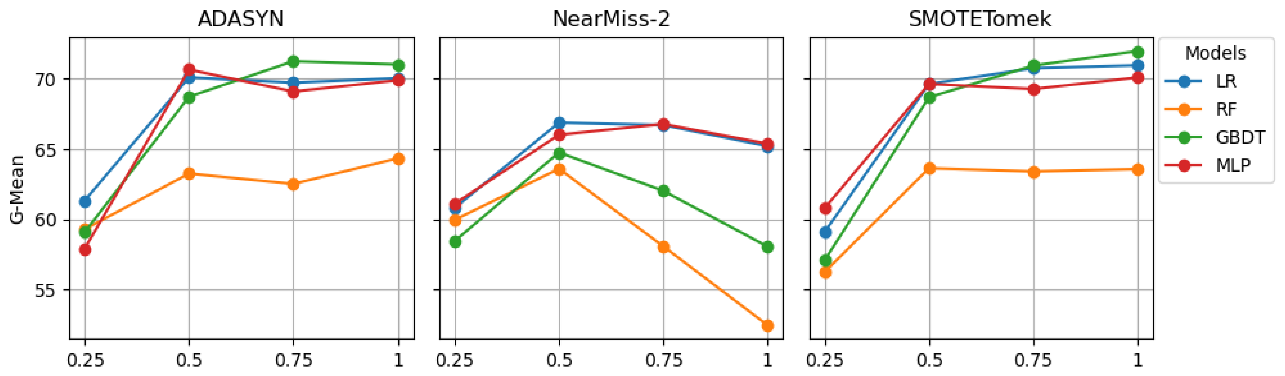
When examining the optimal combination of a machine learning model and a sampling approach, the results obtained on the resampled ODS indicated that the GBDT model tends to outperform LR, RF, and MLP when resampling is carried out using ADASYN and SMOTETomek. The optimal sampling ratio with ADASYN was 0.75, while with SMOTETomek, the optimal sampling ratios were 0.75 and 1. Conversely, when resampling was conducted using NearMiss-2, the G-Mean scores suggest that LR is likely to perform well, with an optimal sampling ratio of 0.50, while the AUC scores indicate that the MLP model is more likely to excel with an optimal sampling ratio of 0.25.

Addressing the effectiveness of different models on the resampled CUDS, the G-Mean scores suggested that the GBDT model was the best choice for ADASYN resampling, with an optimal sampling ratio of 0.75. However, the AUC scores favored the MLP model, suggesting its superiority with an optimal sampling ratio of 0.50. In the case of SMOTETomek, both the G-Mean and AUC scores favored the GBDT model as the optimal choice at a sampling ratio of one. On the other hand, for the CUDS resampled by NearMiss-2, both the G-Mean and AUC scores indicate that the LR model is likely to perform the best, especially at a sampling ratio of 0.50. These findings provide valuable insights into the interplay between the machine learning models, sampling approaches, and optimal ratios for addressing class imbalance in crash severity analysis.

Resampling the ODS using ADASYN and SMOTETomek revealed that increasing the sampling ratio from 0.25 to 0.75 significantly enhanced the performance of LR, GBDT, and MLP, while the increase in performance for RF was comparatively more gradual. Furthermore, increasing the sampling ratio from 0.75 to 1 did not result in a substantial change in the models’ performance. In the case of resampling the ODS using NearMiss-2, raising the sampling ratio from 0.25 to 0.50 is likely to improve model performance. However, increasing the ratio from 0.50 to 1 led to a pronounced reduction in the models’ effectiveness. In general, the performances of models are expected to decrease as the number of observations for training decline.

Similar trends were observed when resampling the CUDS using ADASYN and SMOTETomek. Increasing the sampling ratio from 0.25 to 0.50 significantly improved the performance of LR, GBDT, and MLP. The impact of changes in the sampling ratios for resampling the CUDS using NearMiss-2 mirrored that of the ODS. These findings shed light on the nuanced effects of varying sampling ratios on different machine learning models, providing valuable insights for optimizing the handling of class imbalance in crash severity analysis.

6. Conclusions

This study makes a significant contribution by introducing a novel cluster-based under-sampling technique, incorporating the same distance function as in k-prototypes clustering for calculating the distances between major and minor injury observations. Furthermore, the findings highlighted that the combination of cluster-based under-sampling and explored sampling approaches substantially improves the performance of machine learning models. In addition, our results indicate that ADASYN and SMOTETomek enhance model performance to a similar level and are likely to outperform NearMiss-2. Notably, the GBDT model is likely to perform well on crash data resampled by ADASYN and SMOTETomek, while the LR model is preferable with NearMiss-2. Lastly, increasing the sampling ratio while applying ADASYN and SMOTETomek is likely to enhance the performance of models up to a certain level, while with NearMiss-2, the performance is likely to drop significantly after a certain point. This comparative study may work as a reference for future road safety researchers and analysts to choose an appropriate combination of sampling approaches and machine learning models. Authorities and individuals interested in discovering more accurate estimations of the key factors of crash severity may also utilize the proposed cluster-based sampling approaches.

Like any other study, this study also has some limitations. First of all, this study opted for a binary formation regarding crash severity, where major injury crashes constituted both severe and fatal injuries. A multi-class formation is also a viable approach and may yield different results when the proposed cluster-based under-sampling technique is applied. Secondly, only three sampling approaches were tested in this study. Future researchers can use more novel variants of under-sampling and over-sampling approaches. In addition, they may compare the proposed cluster-based under-sampling technique with existing cluster-based under-sampling techniques. Also, future researchers can opt for more advanced machine learning models such as convolutional neural networks and XGBoost. Lastly, the distribution of major and minor injury crashes in the collected crash data was not extremely imbalanced. The proposed cluster-based under-sampling technique should be tested on more imbalanced data set.

References

1. Bureau of Transportation Statistics. Freight Figures and Facts 2017; Technical Report; United States Department of Transportation: Washington, DC, USA, 2017.
2. Federal Motor Carrier Safety Administration Analysis Division. Large Truck and Bus Crash Facts 2020; Technical Report; United States Department of Transportation: Washington, DC, USA, 2020.
3. Batista, G.E.d.A.P.A.; Bazzan, A.L.C.; Monard, M.C. Balancing training data for automated annotation of keywords: A case study. In Proceedings of the 2003 Workshop on Open-Source Information Systems (WOB’03), Rio de Janeiro, Brazil, 3–5 December 2003; pp. 10–19. [Google Scholar]
4. Devi, D.; Biswas, S.K.; Purkayastha, B. A Review on Solution to Class Imbalance Problem: Undersampling Approaches. In Proceedings of the 2020 International Conference on Computational Performance Evaluation (ComPE), Shillong, India, 2–4 July 2020. [Google Scholar] [CrossRef]
5. Hasanin, T.; Khoshgoftaar, T.M.; Leevy, J.L.; Bauder, R.A. Severely imbalanced Big Data challenges: Investigating data sampling approaches. J. Big Data 2019, 6, 107. [Google Scholar] [CrossRef]
6. Haixiang, G.; Yijing, L.; Shang, J.; Mingyun, G.; Yuanyue, H.; Bing, G. Learning from class-imbalanced data: Review of methods and applications. Expert Syst. Appl. 2017, 73, 220–239. [Google Scholar] [CrossRef]
7. Leevy, J.L.; Khoshgoftaar, T.M.; Bauder, R.A.; Seliya, N. A survey on addressing high-class imbalance in big data. J. Big Data 2018, 5, 1–30. [Google Scholar] [CrossRef]
8. Onan, A. Consensus clustering-based undersampling approach to imbalanced learning. Sci. Program. 2019, 2019, 5901087. [Google Scholar] [CrossRef]
9. Yen, S.J.; Lee, Y.S. Cluster-based under-sampling approaches for imbalanced data distributions. Expert Syst. Appl. 2009, 36, 5718–5727. [Google Scholar] [CrossRef]
10. Gupta, S.; Jivani, A. A Cluster-based Under-Sampling solution for handling Imbalanced Data. Int. J. Emerg. Technol. 2019, 10, 160–170. [Google Scholar]
11. Akash, A.H.; Mahi, F.F.; Mondal, T.; Rahman, M.N.; Ishrak, I.F.; Rahman, M.A.; Arnob, S.; Alvee, S.M. Clustering-Based Under-Sampling with Normalization in Class-Imbalanced Data. In Proceedings of the 2022 IEEE International Conference on Current Development in Engineering and Technology (CCET), Bhopal, India, 23–24 December 2022; IEEE: New York, NY, USA, 2022; pp. 1–6. [Google Scholar]
12. Liu, B.; Ma, Y.; Wong, C.K. Improving an association rule based classifier. In Proceedings of the Principles of Data Mining and Knowledge Discovery: 4th European Conference, PKDD 2000, Lyon, France, 13–16 September 2000; Springer: Berlin/Heidelberg, Germany, 2000; pp. 504–509. [Google Scholar]
13. Chawla, N.V.; Cieslak, D.A.; Hall, L.O.; Joshi, A. Automatically countering imbalance and its empirical relationship to cost. Data Min. Knowl. Discov. 2008, 17, 225–252. [Google Scholar] [CrossRef]
14. Galar, M.; Fernandez, A.; Barrenechea, E.; Bustince, H.; Herrera, F. A review on ensembles for the class imbalance problem: Bagging-, boosting-, and hybrid-based approaches. IEEE Trans. Syst. Man Cybern. Part C Appl. Rev. 2011, 42, 463–484. [Google Scholar] [CrossRef]
15. Mohammadpour, S.I.; Khedmati, M.; Zada, M.J.H. Classification of truck-involved crash severity: Dealing with missing, imbalanced, and high dimensional safety data. PLoS ONE 2023, 18, e0281901. [Google Scholar] [CrossRef]
16. Jeong, H.; Jang, Y.; Bowman, P.J.; Masoud, N. Classification of motor vehicle crash injury severity: A hybrid approach for imbalanced data. Accid. Anal. Prev. 2018, 120, 250–261. [Google Scholar] [CrossRef]
17. Fiorentini, N.; Losa, M. Handling imbalanced data in road crash severity prediction by machine learning algorithms. Infrastructures 2020, 5, 61. [Google Scholar] [CrossRef]
18. Morris, C.; Yang, J.J. Effectiveness of resampling methods in coping with imbalanced crash data: Crash type analysis and predictive modeling. Accid. Anal. Prev. 2021, 159, 106240. [Google Scholar] [CrossRef] [PubMed]
19. Jiang, L.; Xie, Y.; Wen, X.; Ren, T. Modeling highly imbalanced crash severity data by ensemble methods and global sensitivity analysis. J. Transp. Saf. Secur. 2022, 14, 562–584. [Google Scholar] [CrossRef]
20. Barua, S.; Islam, M.M.; Yao, X.; Murase, K. MWMOTE—Majority weighted minority oversampling technique for imbalanced data set learning. IEEE Trans. Knowl. Data Eng. 2012, 26, 405–425. [Google Scholar] [CrossRef]
21. AlMamlook, R.E.; Kwayu, K.M.; Alkasisbeh, M.R.; Frefer, A.A. Comparison of machine learning algorithms for predicting traffic accident severity. In Proceedings of the 2019 IEEE Jordan International Joint Conference on Electrical Engineering and Information Technology (JEEIT), Amman, Jordan, 9–11 April 2019; IEEE: New York, NY, USA, 2019; pp. 272–276. [Google Scholar]
22. Savolainen, P.T.; Mannering, F.L.; Lord, D.; Quddus, M.A. The statistical analysis of highway crash-injury severities: A review and assessment of methodological alternatives. Accid. Anal. Prev. 2011, 43, 1666–1676. [Google Scholar] [CrossRef] [PubMed]
23. Al Mamlook, R.E.; Abdulhameed, T.Z.; Hasan, R.; Al-Shaikhli, H.I.; Mohammed, I.; Tabatabai, S. Utilizing machine learning models to predict the car crash injury severity among elderly drivers. In Proceedings of the 2020 IEEE International Conference on Electro Information Technology (EIT), Naperville, IL, USA, 31 July–1 August 2020; IEEE: New York, NY, USA, 2020; pp. 105–111. [Google Scholar]
24. Haq, M.T.; Zlatkovic, M.; Ksaibati, K. Occupant injury severity in passenger car-truck collisions on interstate 80 in Wyoming: A Hamiltonian Monte Carlo Markov Chain Bayesian inference approach. J. Transp. Saf. Secur. 2022, 14, 498–522. [Google Scholar] [CrossRef]
25. Ahmadi, A.; Jahangiri, A.; Berardi, V.; Machiani, S.G. Crash severity analysis of rear-end crashes in California using statistical and machine learning classification methods. J. Transp. Saf. Secur. 2020, 12, 522–546. [Google Scholar] [CrossRef]
26. Chang, L.Y.; Chien, J.T. Analysis of driver injury severity in truck-involved accidents using a non-parametric classification tree model. Saf. Sci. 2013, 51, 17–22. [Google Scholar] [CrossRef]
27. Zhang, J.; Li, Z.; Pu, Z.; Xu, C. Comparing prediction performance for crash injury severity among various machine learning and statistical methods. IEEE Access 2018, 6, 60079–60087. [Google Scholar] [CrossRef]
28. Wahab, L.; Jiang, H. Severity prediction of motorcycle crashes with machine learning methods. Int. J. Crashworthiness 2020, 25, 485–492. [Google Scholar] [CrossRef]
29. Tang, J.; Liang, J.; Han, C.; Li, Z.; Huang, H. Crash injury severity analysis using a two-layer Stacking framework. Accid. Anal. Prev. 2019, 122, 226–238. [Google Scholar] [CrossRef]
30. Lee, J.; Yoon, T.; Kwon, S.; Lee, J. Model evaluation for forecasting traffic accident severity in rainy seasons using machine learning algorithms: Seoul city study. Appl. Sci. 2019, 10, 129. [Google Scholar] [CrossRef]
31. Zheng, Z.; Lu, P.; Lantz, B. Commercial truck crash injury severity analysis using gradient boosting data mining model. J. Saf. Res. 2018, 65, 115–124. [Google Scholar] [CrossRef] [PubMed]
32. Li, Z.; Liu, P.; Wang, W.; Xu, C. Using support vector machine models for crash injury severity analysis. Accid. Anal. Prev. 2012, 45, 478–486. [Google Scholar] [CrossRef]
33. Singh, J.; Singh, G.; Singh, P.; Kaur, M. Evaluation and classification of road accidents using machine learning techniques. In Proceedings of the Emerging Research in Computing, Information, Communication and Applications: ERCICA 2018, Bangalore, India, 24–25 February 2018; Springer: Berlin/Heidelberg, Germany, 2019; Volume 1, pp. 193–204. [Google Scholar]
34. Kumeda, B.; Zhang, F.; Zhou, F.; Hussain, S.; Almasri, A.; Assefa, M. Classification of road traffic accident data using machine learning algorithms. In Proceedings of the 2019 IEEE 11th International Conference on Communication Software and Networks (ICCSN), Chongqing, China, 12–15 June 2019; IEEE: New York, NY, USA, 2019; pp. 682–687. [Google Scholar]
35. Taamneh, M.; Taamneh, S.; Alkheder, S. Clustering-based classification of road traffic accidents using hierarchical clustering and artificial neural networks. Int. J. Inj. Control Saf. Promot. 2017, 24, 388–395. [Google Scholar] [CrossRef]
36. Infante, P.; Jacinto, G.; Afonso, A.; Rego, L.; Nogueira, V.; Quaresma, P.; Saias, J.; Silva, M.; Costa, R.; Gois, P.; et al. Comparison of Statistical and Machine-Learning Models on Road Traffic Accident Severity Classification. Computers 2022, 11, 80. [Google Scholar] [CrossRef]
37. Iranitalab, A.; Khattak, A. Comparison of four statistical and machine learning methods for crash severity prediction. Accid. Anal. Prev. 2017, 108, 27–36. [Google Scholar] [CrossRef] [PubMed]
38. Song, L.; Fan, W. Combined latent class and partial proportional odds model approach to exploring the heterogeneities in truck-involved severities at cross and T-intersections. Accid. Anal. Prev. 2020, 144, 105638. [Google Scholar] [CrossRef]
39. De Ona, J.; López, G.; Mujalli, R.; Calvo, F.J. Analysis of traffic accidents on rural highways using Latent Class Clustering and Bayesian Networks. Accid. Anal. Prev. 2013, 51, 1–10. [Google Scholar] [CrossRef]
40. Nandurge, P.A.; Dharwadkar, N.V. Analyzing road accident data using machine learning paradigms. In Proceedings of the 2017 International Conference on I-SMAC (IoT in Social, Mobile, Analytics and Cloud) (I-SMAC), Palladam, India, 10–11 February 2017; IEEE: New York, NY, USA, 2017; pp. 604–610. [Google Scholar]
41. Tiwari, P.; Kalitin, D. A Conjoint Analysis of Road Accident Data using K-modes Clustering and sayesian Networks (Road Accident Analysis using clustering and classification). In Proceedings of the Second International Conference on Research in Intelligent and Computing in Engineering, Telangana, India, 25–27 September 2017. [Google Scholar]
42. National Center for Statistics and Analysis. Crash Report Sampling System CRSS Analytical User’s Manual 2016–2019; Technical Report; National Highway Traffic Safety Administration: Washington, DC, USA, 2020.
43. Pahukula, J.; Hernandez, S.; Unnikrishnan, A. A time of day analysis of crashes involving large trucks in urban areas. Accid. Anal. Prev. 2015, 75, 155–163. [Google Scholar] [CrossRef]
44. Al-Bdairi, N.S.S.; Hernandez, S. An empirical analysis of run-off-road injury severity crashes involving large trucks. Accid. Anal. Prev. 2017, 102, 93–100. [Google Scholar] [CrossRef] [PubMed]
45. Al-Bdairi, N.S.S.; Hernandez, S.; Anderson, J. Contributing Factors to Run-Off-Road Crashes Involving Large Trucks under Lighted and Dark Conditions. J. Transp. Eng. Part A Syst. 2018, 144, 04017066. [Google Scholar] [CrossRef]
46. Huang, Z. Extensions to the k-means algorithm for clustering large data sets with categorical values. Data Min. Knowl. Discov. 1998, 2, 283–304. [Google Scholar] [CrossRef]
47. He, H.; Bai, Y.; Garcia, E.A.; Li, S. ADASYN: Adaptive synthetic sampling approach for imbalanced learning. In Proceedings of the 2008 IEEE International Joint Conference on Neural Networks (IEEE World Congress on Computational Intelligence), Hong Kong, China, 1–8 June 2008. [Google Scholar] [CrossRef]
48. Mani, I.; Zhang, I. kNN approach to unbalanced data distributions: A case study involving information extraction. In Proceedings of the Workshop on Learning from Imbalanced Datasets, Washington, DC, USA, 21 August 2003; ICML: Baltimore, MA, USA, 2003; Volume 126, pp. 1–7. [Google Scholar]
49. Chawla, N.V.; Bowyer, K.W.; Hall, L.O.; Kegelmeyer, W.P. SMOTE: Synthetic minority over-sampling technique. J. Artif. Intell. Res. 2002, 16, 321–357. [Google Scholar] [CrossRef]
50. Tomek, I. Two modifications of CNN. IEEE Trans. Syst. Man Cybern. 1976, 6, 769–772. [Google Scholar]
51. Berkson, J. Application of the logistic function to bio-assay. J. Am. Stat. Assoc. 1944, 39, 357–365. [Google Scholar]
52. Breiman, L. Random forests. Mach. Learn. 2001, 45, 5–32. [Google Scholar] [CrossRef]
53. Elyassami, S.; Hamid, Y.; Habuza, T. Road crashes analysis and prediction using gradient boosted and random forest trees. In Proceedings of the 2020 6th IEEE Congress on Information Science and Technology (CiSt), Agadir-Essaouira, Morocco, 12–18 December 2021; IEEE: New York, NY, USA, 2021; pp. 520–525. [Google Scholar]
54. Haykin, S.S. Neural Networks and Learning; Chapter 4: Multilayer Perceptrons; Pearson Education: London, UK, 2009. [Google Scholar]
55. Loyola-González, O.; Martínez-Trinidad, J.F.; Carrasco-Ochoa, J.A.; García-Borroto, M. Study of the impact of resampling methods for contrast pattern based classifiers in imbalanced databases. Neurocomputing 2016, 175, 935–947. [Google Scholar] [CrossRef]
56. Seliya, N.; Khoshgoftaar, T.M.; Van Hulse, J. A study on the relationships of classifier performance metrics. In Proceedings of the 2009 21st IEEE International Conference on Tools with Artificial Intelligence, Newark, NJ, USA, 2–4 November 2009; IEEE: New York, NY, USA, 2009; pp. 59–66. [Google Scholar]
57. Bradley, A.P. The use of the area under the ROC curve in the evaluation of machine learning algorithms. Pattern Recognit. 1997, 30, 1145–1159. [Google Scholar] [CrossRef]
58. Pedregosa, F.; Varoquaux, G.; Gramfort, A.; Michel, V.; Thirion, B.; Grisel, O.; Blondel, M.; Prettenhofer, P.; Weiss, R.; Dubourg, V.; et al. Scikit-learn: Machine learning in Python. J. Mach. Learn. Res. 2011, 12, 2825–2830. [Google Scholar]
Figure 1. Workflow for the application of cluster-based under-sampling coupled with different sampling approaches.
Information 15 00145 g001
Figure 2. Optimal number for clustering.
Information 15 00145 g002
Figure 3. G-Mean scores of models developed on resampled ODS.
Information 15 00145 g003
Figure 4. AUC scores of models developed on resampled ODS.
Information 15 00145 g004
Figure 5. G-Mean scores of models developed on resampled CUDS.
Information 15 00145 g005
Figure 6. AUC scores of models developed on resampled CUDS.
Information 15 00145 g006