Abstract
With the rapid growth of the data scale in data centers, the high reliability of storage is facing various challenges. Specifically, hardware failures such as disk faults occur frequently, causing serious system availability issues. In this context, hardware fault prediction based on AI and big data technologies has become a research hotspot, aiming to guide operation and maintenance personnel to implement preventive replacement through accurate prediction to reduce hardware failure rates. However, existing methods still have weaknesses in terms of accuracy due to the impacts of data quality issues such as the sample imbalance. This article proposes a disk fault prediction method based on classification intensity resampling, which fills the gap between the degree of data imbalance and the actual classification intensity of the task by introducing a base classifier to calculate the classification intensity, thus better preserving the data features of the original dataset. In addition, using ensemble learning methods such as random forests, combined with resampling, an integrated classifier for imbalanced data is developed to further improve the prediction accuracy. Experimental verification shows that compared with traditional methods, the F1-score of disk fault prediction is improved by 6%, and the model training time is also greatly reduced. The fault prediction method proposed in this paper has been applied to approximately 80 disk drives and nearly 40,000 disks in the production environment of a large bank’s data center to guide preventive replacements. Compared to traditional methods, the number of preventive replacements based on our method has decreased by approximately 21%, while the overall disk failure rate remains unchanged, thus demonstrating the effectiveness of our method.
1. Introduction
With the explosive growth of data scale, the high reliability of storage faces enormous challenges as the data foundation carries financially distributed information systems. The disk is the most important medium of storage. The self-monitoring analysis and reporting technology (SMART) of the disk can analyze the working status of the hard disk and detect various attributes of the disk. The main research method is based on feature selection, selecting the main features that affect hard disk fault prediction and then establishing disk fault prediction models using machine learning algorithms such as decision trees, support vector machines, Bayesian networks, and neural networks [1,2,3]. However, standard machine learning models cannot deal with imbalanced data very well. This article proposes a disk fault prediction method based on classification intensity resampling. Considering that in practical applications, even if the imbalance ratio is the same, different datasets may exhibit extremely different classification intensities. By introducing a base classifier to calculate the classification intensity, the gap between the imbalance degree of the dataset and the actual classification intensity of the task is filled, thus better preserving the data features of the original dataset and improving model performance. By integrating ensemble learning methods, such as random forest, with resampling techniques, an ensemble classifier tailored for unbalanced data was ultimately developed, further enhancing prediction accuracy.
2. Research Background
2.1. The Current Research Status
Many distributed information systems rely on large-scale, low-cost, ordinary devices, such as disks, which are prone to hardware failures. These failures often lead to system availability issues, posing challenges to the overall performance and reliability of the system. However, the existing hardware fault prediction methods based on big data and AI technology are limited by issues such as sample imbalance, complex physical characteristics of various hardware, and diverse fault types, resulting in low accuracy and generalization as well as inefficient preventive replacement. The current focus of operation and maintenance and research hotspots include disk fault prediction.
Specifically, disk fault prediction is mainly based on self-monitoring analysis and reporting technology (SMART) analysis, directly predicting the fault state at a certain moment in the future. Microsoft proposed a transfer learning approach [4,5], and some scholars have proposed data-screening methods with deep learning [6,7,8,9,10,11]. Some progress has been made in model accuracy, but it is still difficult to effectively solve the sample imbalance problem caused by scarce fault samples. A comparison of commonly used disk fault prediction methods is shown in Table 1.

Table 1.
Comparison of commonly used disk fault prediction methods.
It can be seen that the aforementioned methods have not fundamentally solved the problem of sample imbalance, limiting accuracy.
2.2. Issues and Challenges
With the explosive growth of data scale, the high reliability of storage, as the data foundation of financial distributed information systems, faces enormous challenges. The disk is the most important medium of storage, and sudden disk failure can directly affect the stable operation of business systems. The SMART analysis of the disk can analyze the working status of the hard disk and detect various attributes of the disk. Currently, the main practice of operation and maintenance personnel is to predict faults based on SMART analysis of the disk and implement preventive replacement to ensure the high reliability of the disk. Currently, the preventive replacement of disks faces a dilemma. On the one hand, if the false positive rate is too high, frequent replacement will lead to resource waste. On the other hand, if the false positive rate is reduced to improve accuracy, there may be omissions, and failure to replace on time may lead to business losses. SMART includes 255 attributes related to hard disk failures, such as temperature, humidity, pressure, the total number of reassigned sectors, and start–stop times. The main research method is based on feature selection, selecting the main features that affect hard disk failure prediction and then establishing a disk failure prediction model through machine learning algorithms, e.g., decision trees, support vector machines, Bayesian networks, and neural networks, to detect hidden problems in advance and improve the reliability of data storage in data centers. Although this method has improved prediction accuracy compared with traditional methods, the F1-score is still insufficient. The main difficulty is that the number of abnormal samples in SMART data is extremely scarce and the categories are imbalanced. Standard machine learning models cannot deal with imbalanced data well. The implicit optimization goal of these models is classification accuracy. However, classification accuracy itself is not a reasonable evaluation index under the conditions of imbalanced categories because it tends to judge all samples as majority classes. In the premise that minority class samples contain more important information, this classifier has poor performance in practical applications.
To solve the problem of class imbalance learning, researchers have proposed a series of solutions, which can be roughly divided into two categories: data-level methods and algorithm-level methods. Data-level methods balance the data distribution or remove noise by adding or deleting samples in the dataset (also known as resampling methods), and the modified dataset is used to train a standard learner. However, conventional random undersampling and SMOTE oversampling techniques based on nearest neighbors have poor performance in preserving the original data features [12,13,14]. As for algorithm-level methods, by modifying existing standard machine learning methods to correct the influence of different class sample sizes on them, standard learning methods can also adapt to imbalanced learning scenarios but rely on specific domain knowledge and have poor practical application effects [15,16].
Considering that in practical applications, even if the imbalance ratio is the same, different datasets may exhibit very different classification intensities. Therefore, how to integrate data-level methods with algorithm-level methods and take into account the classification intensity of data during data resampling is an important yet challenging issue.
3. Model Architecture
This article proposes a disk failure prediction method based on classification intensity resampling. It fills the gap between the imbalance level of the dataset and the actual classification intensity of the task, thus better preserving the data characteristics of the original dataset and maximizing the effectiveness of the model. In addition, using ensemble learning methods such as random forest combined with resampling, we developed an ensemble classifier for imbalanced data to further improve the prediction accuracy.
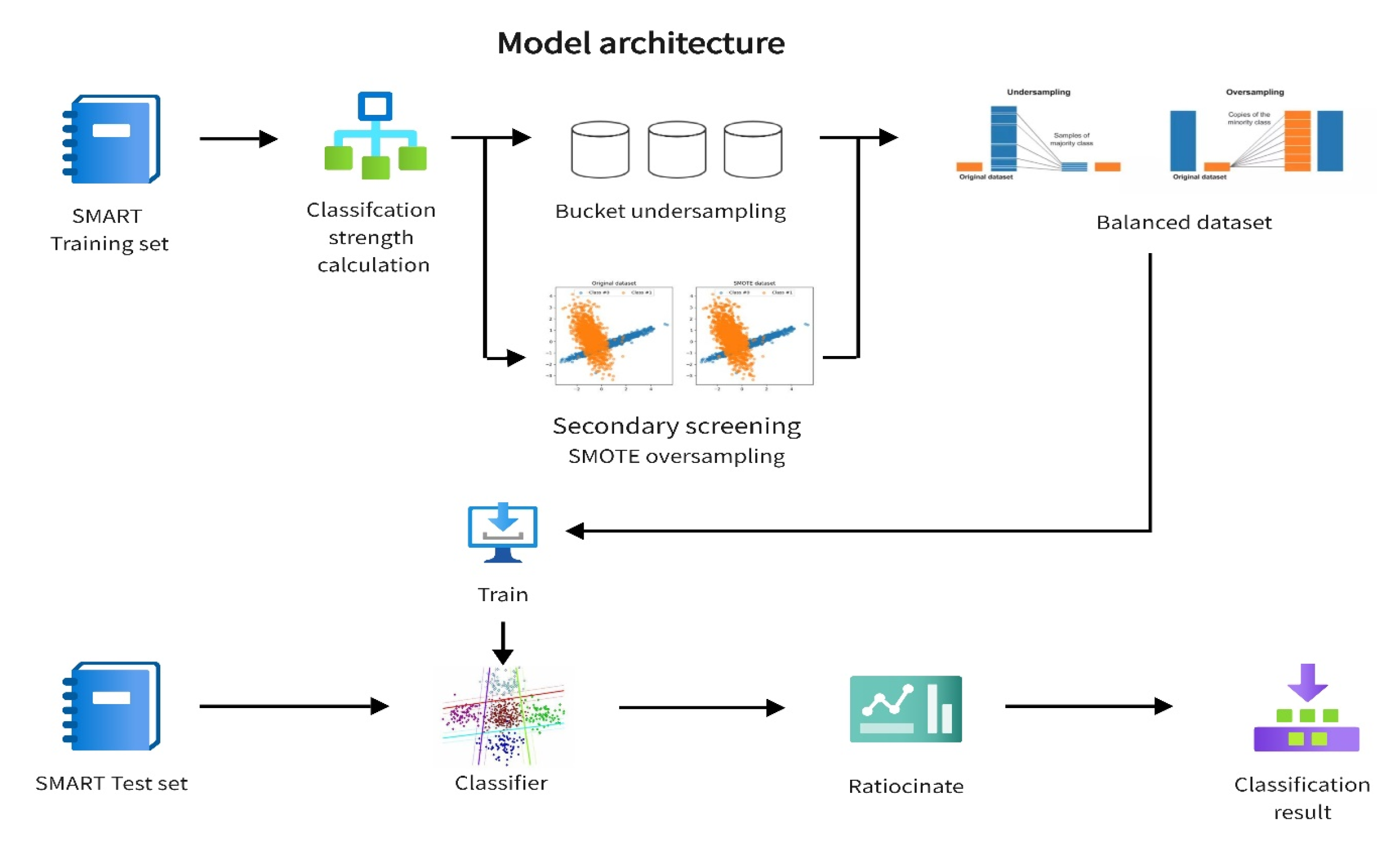
Figure 1 illustrates the architecture of the proposed model which consists of classification intensity calculation based on base classifiers, bucket undersampling, secondary screening SMOTE oversampling, and retraining the base classifier based on balanced datasets.

Figure 1.
Model architecture.
4. Classification Intensity Calculation
Formally, we use F to represent a classifier. For a sample , we use to represent the probability that the classifier outputs a positive sample when inputting x. Due to the minority rate samples being marked as 1 and the majority class samples being marked as 0, classification intensity can be formally defined as probability , since the true label is binary (0 or 1).
The definition of each sample in the imbalanced dataset is as follows: D represents the training set, each sample point is represented by , the minority class is , and the majority class is .
For P, classification intensity means the probability of the minority class samples being hit. This definition represents confidence. When the value is large, it indicates that it is very close to the true label, which has guiding significance for oversampling; For N, classification intensity means the probability of the majority class samples being misjudged. This definition quantifies the difficulty of classification. When the value is large, it indicates a significant difference from the true label, making classification more difficult.
In practical applications, even if the imbalance ratio is the same, different datasets may exhibit extremely different classification difficulties. The classification intensity carries more information about the implicit distribution of the dataset and can better reflect the classification difficulty of the task.
Secondly, classification intensity serves as a bridge between data sampling strategies and classifier learning capabilities. Most existing resampling methods are completely independent of the classifier used. However, different classifiers may have significant performance differences on the same imbalanced data classification task and exhibit completely different behavior patterns. When conducting resampling, the differences in the learning abilities of different models should be taken into account, and the definition of classification intensity implies the information about the learning abilities of different models.
A model considering classification intensity can achieve the following:
- (1)
- Due to the fact that classification intensity is defined by a given learner, the distribution of classification intensity itself varies depending on the learning ability of different classifiers. This enables the model to naturally adapt to the learning process of different classifiers and obtain the optimal optimization process based on the different classification abilities of the learners.
- (2)
- The model can be used to collaborate with any classifier and improve its classification performance on large-scale imbalanced datasets in an integrated manner.
In actual production, our main concern is the classification performance of the classifier on the original imbalanced dataset. Therefore, when evaluating the classification model, we do not resample the dataset, leaving it in a category-imbalanced state. The technical details of classification intensity calculation are presented in Algorithm 1.
| Algorithm 1 Classification intensity calculation |
| Input: Training set D;
Base learner f Output: Initial classifier ;
Sample classification intensity 1. Initialization: minority sample set in , majority sample set in ; 2. Calculate the number of majority and minority samples , ; 3. Using random majority class subsampling to obtain a majority class subset . Make . 4. Using balanced dataset training initial classifier ; 5. Utilize predict the probability of all samples being misjudged in ; 6. Utilize predict the probability of all samples being hitted in ; return |
In this article, a random forest is introduced as the base learner. Random forest is an ensemble learning method based on decision trees and utilizes the results of multiple decision trees for classification or regression. In a random forest, each decision tree classifies or regresses the data and ultimately obtains the final result by averaging or voting the output results of all decision trees. This ensemble learning method effectively avoids the problem of overfitting a single decision tree.
For a dataset with m samples and n features, the random forest algorithm can be constructed by the following steps: Step a. Sample N subsets of the training set. Firstly, bootstrap sampling is performed on the original dataset D to generate N subsets of data with size . At the same time, k features are randomly selected as reference feature sets for decision tree training. Step b. Build a decision tree. Use the CART algorithm (Classification and Regression Tree) to construct a decision tree for each subset until the preset stop conditions (such as tree depth, number of leaf nodes, etc.) are met. Since each decision tree is trained on different subsets of data, each decision tree in a random forest is different. The main advantages of random forests include good model robustness, robustness to missing data, and the ability to handle high-dimensional data. Meanwhile, since random forests can generate feature importance, they can also be used for feature selection.
5. Bucket Undersampling
In the processing of imbalanced datasets, random undersampling is the most commonly used and simplest undersampling method, which mainly achieves undersampling by randomly selecting a portion of the samples from the majority class without any processing for the minority class. When randomly selecting majority class samples, there is randomness, which leads to a decrease or loss of some important information in the majority class. When the data imbalance ratio increases significantly, the loss of important information increases sharply, ultimately leading to a sharp decrease in the comprehensive classification performance of the classifier in imbalanced datasets as the imbalance degree increases.
For majority class samples, classification intensity quantifies the difficulty of classification. When a sample exhibits a high classification intensity value, it indicates greater difficulty in accurate classification, thereby implying a higher informational value and deserving a higher sampling rate. Conversely, a low classification intensity value suggests easier accurate classification, resulting in a lower information density and thus deserving less retention.
The idea of bucketing is analogous to that of a “histogram”. Since classification intensity is expressed as a probability value ranging from 0 to 1, several buckets can be established, each encompassing a specific probability range. For instance, if five buckets are set, the probability range for the first bucket would be 0–0.2; for the second bucket, it would be 0.2–0.4; and so on, with the fifth bucket encompassing the range of 0.8–1. Each sample point is then assigned to the corresponding bucket based on its calculated classification intensity value. Under the approach proposed in this paper, the first bucket, despite containing the largest number of samples, exhibits the lowest classification intensity and thus receives the lowest sampling weight. Conversely, the fifth bucket, containing the samples with the highest classification intensity and the smallest sample size, receives the highest sampling weight.
The main idea of bucket undersampling proposed in this article is to randomly undersample each bucket based on the average classification intensity of each bucket as a weight. Although there are a large number of buckets with low classification intensity, they only need to retain a small portion to represent their corresponding distribution of “skeletons” because they have been well classified by the base classifier, which is used to prevent the learner from being affected by noise in a few classes.
However, since the classifier has already learned such samples well, the majority of them can be discarded in subsequent training since the weight is relatively small. The stronger the classification intensity of the bucket, the higher the weight and the more samples are sampled. The sample points in this bucket may be closer to the classification boundary, making it difficult for the base classifier to recognize. From the perspective of information extraction, this type of sample has the largest amount of information during model training and should be retained more. Therefore, compared to random undersampling, bucket-based undersampling can better preserve the most valuable information in the original dataset without losing the “skeleton” of data distribution. The technical details of bucket undersampling are presented in Algorithm 2.
| Algorithm 2 Bucket undersampling |
| Input: Majority class sample set N;
Number of buckets divided k; Majority sample classification intensity ; Output: Sample set N after sub-bucket undersampling 1. Determine the probability numerical interval for each sub-bucket with the interval for the i-th bucket 2. Based on distribution, according to the interval of buckets, load each sample point into k buckets, and the samples in each bucket are 3. Calculate the average classification intensity of each bucket with the average classification intensity of the i-th bucket ; 4. Calculate the sampling weight of each bucket, and the sampling weight of the i-th bucket is ; 5. Randomly sample each bucket based on its sampling weight with the i-th bucket having a sampling amount of ; return Return the sample set after sub-bucket undersampling |
6. Secondary Screening SMOTE Oversampling
By simply copying a few class samples to achieve sample increase, random oversampling makes it easy to make the model classification area too specific, resulting in insufficient generalization and ultimately leading to overfitting of the model classification [17].
The SMOTE (Synthetic Minority Oversampling Technique) algorithm is an improved method for random oversampling, which is currently widely used. It creates minority class samples through synthesis instead of simply copying minority classes to achieve oversampling. The technical details of SMOTE oversampling are presented in Algorithm 3.
| Algorithm 3 SMOTE oversampling |
| Input: minority sample x;
x’s adjacent sample set X Output: New Sample 1. Repeat until the required oversampling rate is completed do 2. Calculate the distance between the minority sample x and its k-nearest neighbors and randomly select a neighbor sample 3. Randomly specify proportions 4. Combining x and Two samples, according to Synthesize new sample 5. End repeat return Return New Sample |
SMOTE randomly synthesizes a few instances along the line connecting them and their selected nearest neighbors, ignoring the nearby majority instances, which can easily blur the boundaries of minority class samples and reduce the accuracy of the algorithm [18]. For minority class samples, a high classification intensity value indicates closer proximity to the true label, representing a higher degree of confidence. Drawing inspiration from the concept of “semi-supervision”, we calculate the classification intensity for the oversampled points randomly generated by SMOTE and retain those with higher confidence, thereby enhancing the performance of oversampling.
The main idea of the secondary screening SMOTE oversampling method proposed in this article is to use a base classifier to calculate the classification intensity of each sample point for the samples generated by SMOTE, ensuring that it is not lower than the average classification intensity of minority class samples. By performing secondary screening on SMOTE and retaining sample points with high reliability, oversampling compared to standard SMOTE can effectively reduce the disturbance of noise points on classification boundaries and avoid algorithm overfitting. The technical details of secondary screening oversampling are presented in Algorithm 4.
| Algorithm 4 Secondary screening oversampling |
| Input: minority class sample set P;
Oversampling rate R; Minority sample classification intensity ; Initial classifier Output: oversampled dataset 1. Calculate the average classification intensity of minority class samples 2. Based on the oversampling rate R, use SMOTE to oversample P and obtain the sampling dataset ; 3. Calculate the classification intensity f for each sample in the oversampling dataset ; 4. Keep Sample points with form an oversampling dataset return Return oversampled datase ; |
7. Classifier Training
For the classifier training, the above sampling methods can be flexibly selected based on the imbalance ratio of the original dataset, and the final balanced dataset can be constructed. Through actual data verification, when the imbalance ratio of the original dataset is within 100, only sub-bucket undersampling is used. When the imbalance ratio is greater than 100, it is recommended to use both bucket undersampling and secondary screening SMOTE oversampling to construct a balanced dataset. Afterwards, based on the constructed balanced dataset, the base classifier is retrained to obtain the final prediction model. The technical details of classifier training are presented in Algorithm 5.
| Algorithm 5 Classifier Training |
| Input: Dataset imbalance ratio ;
Undersampled dataset ; Oversampling dataset ; Classifier f Output: Final classifier 1. If then 2. Only using bucket undersampling method to construct a balanced dataset ; 3. Else if then 4. Using bucket undersampling and secondary screening SMOTE oversampling methods to construct a balanced dataset ; 5. End if 6. Train classifier f using a balanced dataset to obtain the final classifier return Return ; |
8. Experiment and Analysis
The innovation of this model lies in the novel undersampling and oversampling methods proposed, and the balanced dataset constructed can better reflect the information of the source data, thus achieving better prediction results. Therefore, the focus of the experimental analysis is verifying the effectiveness of bucket undersampling and secondary screening SMOTE oversampling through actual data and analyze and compare the optimal combination usage strategy of this model.
Based on this, the experiment considers three types of evaluation scenarios, including the evaluation of the effects of bucket undersampling and random undersampling; the evaluation of the effects of secondary screening SMOTE oversampling and SMOTE oversampling; and the evaluation of the effects of bucket undersampling alone, secondary screening SMOTE oversampling alone, and mixed sampling.
8.1. Experimental Environment
Number of Servers: 1; Server Model: Intel(R) Xeon E5-2650v2 specifications: CPU@2.60 GHz with 32 GB RAM; Operating System: CentOS 7.3; Programming Language: Python; Experimental Tool: Jupyter notebook.
8.2. Datasets
This article uses two types of datasets. The first is the SMART dataset [19], which is sourced from the hard drive model ST31000524NS manufactured by Seagate. This dataset is a public dataset with existing faulty disk labels, and 11 features are selected through feature selection. The ones marked with ’raw’ are the original values of the attributes, as shown in Table 2. Randomly select a certain number of minority and majority class samples from the dataset to construct experimental sets with different imbalances. The basic information is shown in Table 3. The purpose is to compare the effectiveness of resampling methods in various imbalanced datasets.
Table 2.
SMART dataset properties.
Table 3.
SMART datasets with different unbalance ratios.
The second type of dataset [20,21] has different imbalanced ratios and can further verify the generalization of the methods in this article. In addition to being used for disk SMART data, it is also applicable to other imbalanced and classified datasets. Please refer to Table 4 for details.
Table 4.
Other imbalanced datasets.
8.3. Evaluating Indicator
Table 5 presents the confusion matrix of the binary classification results with the first column showing the actual labels of the samples and the first row showing the predicted labels of the samples. Among them, TP (True Positive), TN (True Negative), FP (False Positive), and FN (False Negative) are composed of four values, where TP is the positive example of correct classification, TN is the negative example of correct classification, FP is the positive example of incorrect classification, and FN is the negative example of incorrect classification.
Table 5.
Confusion matrix for binary classification problems.
Based on the confusion matrix, this article evaluates the performance of classification models on imbalanced datasets using three indicators, i.e., recall, precision, and F1-score, as described below.
For the binary classification of imbalanced datasets, we hope that as many positive samples can be detected as possible to ensure that the model has a high recall rate in this case. The higher the value, the greater the recall and precision rates of the current classification algorithm, indicating better classification performance. Compared to accuracy, is more suitable for evaluating the classification performance of imbalanced datasets.
8.4. Experimental Plan and Analysis
This article of the experiment is based on the two types of datasets mentioned above, and the specific parameters in the experiment are set as follows. The seed used to generate a random number generator in a random forest is set to 0. The sub-bucket undersampling method sets the number of sub-buckets to 10 each time, and the secondary screening oversampling method extracts five samples each time to construct new samples based on SMOTE. The experimental evaluation indicators Recall, Precision, and F1-score are obtained by simulating 100 mean values with random forest parameters defaulted. To better compare the computational complexity and time consumption of algorithms, the experimental time was obtained by averaging 1000 simulations of the model.
We designed three comparative analysis scenarios, namely the comparison between bucket undersampling and random undersampling, the comparative analysis between the secondary screening SMOTE oversampling and standard SMOTE oversampling, and the comprehensive comparative analysis.
- (1)
- Comparative analysis of bucket undersampling and random undersampling
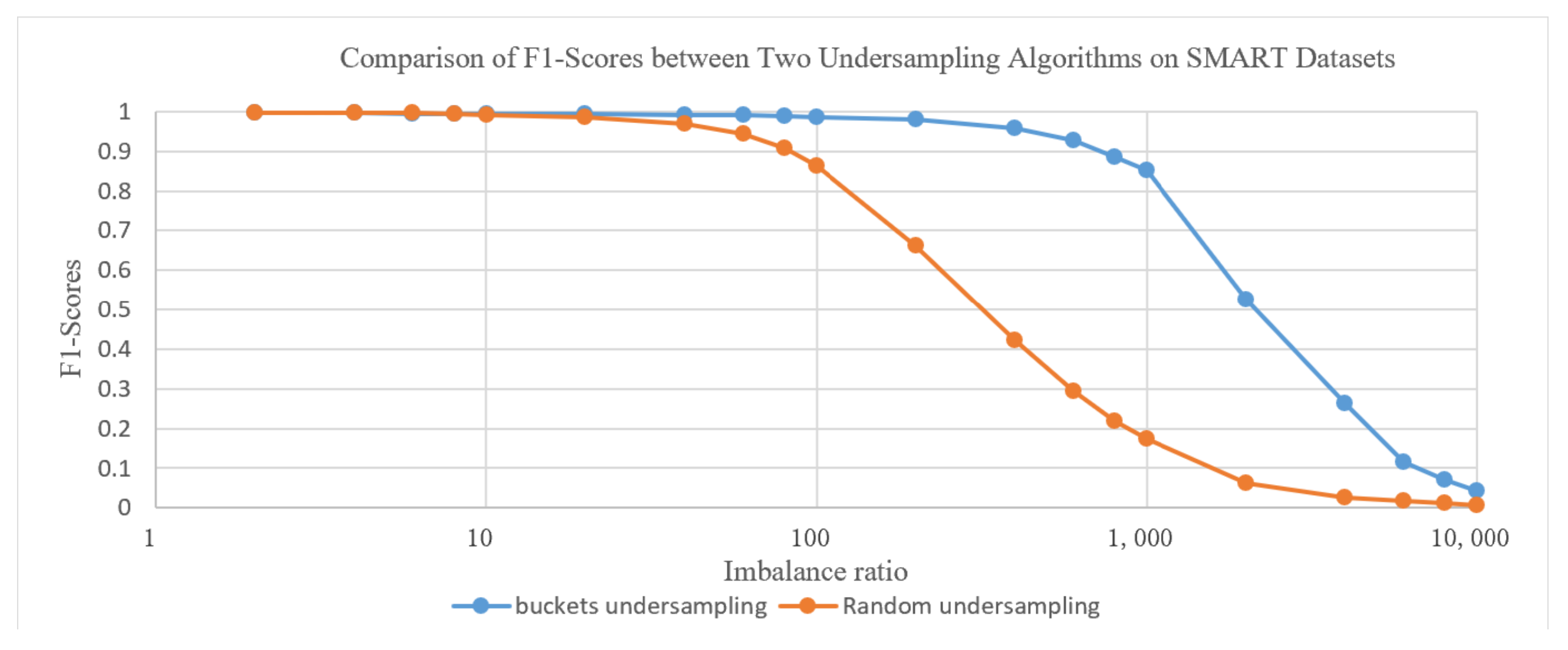
Figure 2 shows the comparison of F1 values between bucket undersampling and random undersampling algorithms on SMART datasets with different balance ratios. As the imbalance ratio increases, the F1 value of bucket undersampling is significantly higher than that of random undersampling.
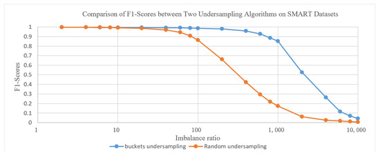
Figure 2.
Comparison of cost–time between two undersampling algorithms on SMART datasets.
Figure 3 shows the comparison of cost–time between two undersampling algorithms on SMART datasets with different balance ratios. The cost–time of bucket-based undersampling has been slightly increased compared to random undersampling, but it is still on the same order of magnitude.
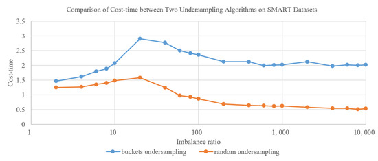
Figure 3.
Comparison of cost–time between two undersampling algorithms on SMART datasets.
The detailed performance comparison on other imbalanced datasets shows similar conclusions, as shown in Table 6.
Table 6.
Comparison of perf between two undersampling algorithms on other imbalanced datasets.
- (2)
- Comparative analysis of secondary screening SMOTE oversampling and standard SMOTE oversampling
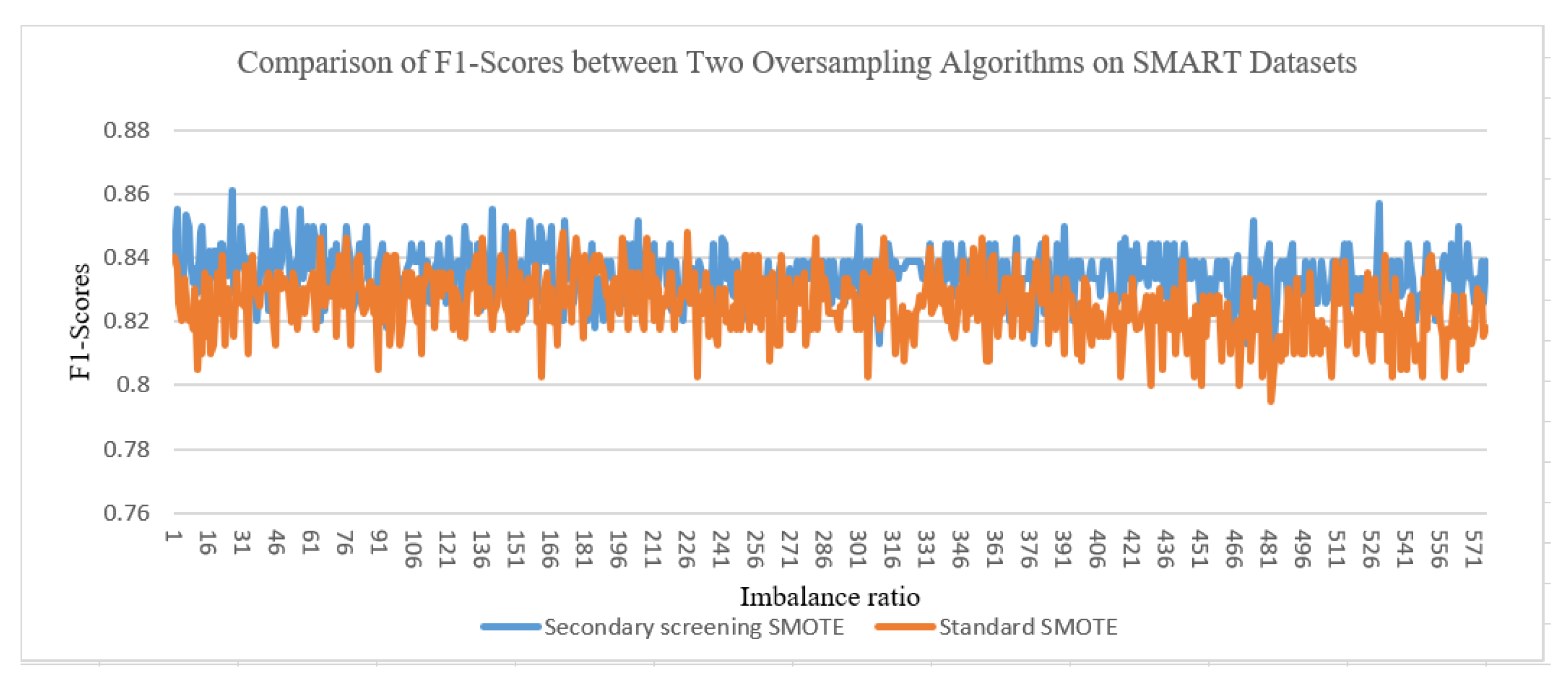
From Figure 4, on SMART datasets with different imbalanced ratios, the secondary screening SMOTE algorithm has an average F1 value 2% higher than the standard SMOTE algorithm.
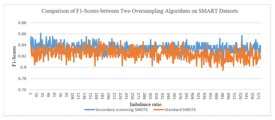
Figure 4.
Comparison of F1-scores between two oversampling algorithms on SMART datasets.
- (3)
- Comprehensive comparative analysis
The bucket undersampling and secondary screening SMOTE oversampling methods in this article can correspond to three combinations in practical applications:
- Only using sub-bucket undersampling;
- Only using secondary screening SMOTE oversampling;
- Simultaneous using bucket undersampling and secondary screening SMOTE oversampling
Through analysis and comparison, we can derive efficient combination strategies to guide the maximum effectiveness of the model in practical applications.
Figure 5 shows the F1 value comparison of the above three types of combination methods on the SMART dataset. From the graph, we can see that when the imbalance ratio of the dataset is below 100, the performance of the three types of methods is similar. However, due to the low time complexity of sub-bucket undersampling and the short training time of the sampled model, it is more suitable to directly use sub-bucket undersampling processing. When the imbalance of the dataset continues to increase, the F1 value of sub-bucket undersampling significantly decreases, and the performance of the other two methods is similar.
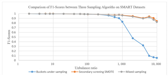
Figure 5.
Comparison of F1-scores between three sampling algorithms on SMART datasets.
However, due to the use of only secondary screening SMOTE, the training set size will expand and the training time will be longer. Overall, mixed sampling is more suitable in such scenarios.
Table 7 and Table 8 show the experimental results on other imbalanced binary classification datasets, which also support the above conclusion and demonstrate the generalization of the method.
Table 7.
Comparison of F1-scores between three sampling algorithms on other imbalanced datasets.
Table 8.
Comparison of cost–time between three sampling algorithms on other imbalanced datasets.
- (4)
- Experimental Conclusion
Based on the experimental results above, compared with random undersampling, the F1-score of bucket undersampling increases rapidly with the increase in the data imbalance ratio. Compared with the standard SMOTE oversampling method, the F1-score of the secondary screening SMOTE oversampling method increases by 2%. Compared with directly training on the original dataset, using the resampling method classifier in this paper, the F1-score increases by 6%, and the model training time is significantly reduced.
The sampling method proposed in this article has strong generalization ability. Among them, bucket undersampling is suitable for scenarios with an imbalance ratio of less than 100, and mixed sampling (bucket undersampling and secondary screening SMOTE oversampling) is suitable for scenarios with an imbalance ratio between 100 and 10,000. Due to the construction of a small-scale balanced dataset through undersampling, the training time is significantly compressed while ensuring accuracy such as F1-score, resulting in better performance.
8.5. Application Effect Analysis
This model has been deployed in a production environment of a bank, and it has been applied to fault prediction for approximately 80 mid-to-high-end disk drives with nearly 40,000 disks. A centralized disk management tool has also been developed to support it. It can generate weekly health check reports, covering SMART analysis and the prediction results of disks, assisting in prompting front-line operation and maintenance personnel to identify potential problems and guide preventive replacement, achieving good results.
9. Conclusions
Most existing methods for disk fault prediction are based on SMART data. They first select the main features that affect hard disk fault prediction and then establish a disk fault prediction model through machine learning algorithms such as decision trees, support vector machines, Bayesian networks, and neural networks. However, these methods cannot cope well with imbalanced data. This article proposes a disk fault prediction method based on classification intensity resampling. By introducing a base classifier to calculate the classification intensity, the gap between the imbalance degree of the dataset and the actual classification intensity of the task is filled, and the data features of the original dataset are better preserved. In addition, the use of ensemble learning methods such as random forests, combined with resampling, ultimately results in an ensemble classifier for imbalanced data, further improving the prediction accuracy. The proposed method first trains the base classifier to calculate sample classification intensity; then, it begins bucket undersampling and secondary screening SMOTE oversampling, and finally, it retrains the base classifier based on a balanced dataset to obtain the prediction model. After actual data validation, bucket undersampling is more effective than random undersampling, and the S score accelerates with the increase of the data imbalance ratio. The second screening SMOTE oversampling method improves the -score by 2% compared with the standard SMOTE oversampling method. Compared with direct training on the original dataset, using the resampling method in this article improves the classifier F1-score by 6%, and the model training time was significantly reduced.
The method in this article uses a single sampling during the sampling stage, which has a certain degree of randomness. Future work could benefit from improving the model’s stability through iterative and multiple sampling strategies and exploring the integration of reinforcement learning to train a meta-sampler for optimizing the resampling process [22]. Additionally, it proposes investigating the use of advanced base classifiers, such as deep learning models, to further enhance the prediction accuracy and applicability of the disk failure prediction methodology.
Author Contributions
Conceptualization, J.G.; software, S.W.; validation, S.W.; formal analysis, S.W.; investigation, S.W.; writing—original draft, S.W.; writing—review & editing, J.G. All authors have read and agreed to the published version of the manuscript.
Funding
This research received no external funding.
Institutional Review Board Statement
Not applicable.
Informed Consent Statement
Not applicable.
Data Availability Statement
The datasets presented in this article are not readily available because the data are from a 3rd party business.
Conflicts of Interest
The authors declare no conflicts of interest.
References
- Chaves, I.C. Hard Disk Drive Failure Prediction Method Based On A Bayesian Network. In Proceedings of the The International Joint Conference on Neural Networks (IJCNN), Rio de Janeiro, Brazil, 8–13 July 2018. [Google Scholar]
- Zhu, B.; Wang, G.; Liu, X.; Hu, D.; Lin, S.; Ma, J. Proactive drive failure prediction for large scale storage systems. In Proceedings of the IEEE 29th Symposium on Mass Storage Systems and Technologies, MSST 2013, Long Beach, CA, USA, 6–10 May 2013; pp. 1–5. [Google Scholar]
- Aussel, N.; Jaulin, S.; Gandon, G.; Petetin, Y.; Chabridon, S. Predictive models of hard drive failures based on operational data. In Proceedings of the IEEE International Conference on Machine Learning & Applications, Cancun, Mexico, 18–21 December 2017. [Google Scholar]
- Xu, Y.; Sui, K.; Yao, R.; Zhang, H.; Lin, Q.; Dang, Y.; Li, P.; Jiang, K.; Zhang, W.; Lou, J.G.; et al. Improving Service Availability of Cloud Systems by Predicting Disk Error. In Proceedings of the USENIX Annual Technical Conference, Boston, MA, USA, 11–13 July 2018; pp. 481–494. [Google Scholar]
- Botezatu, M.M.; Giurgiu, I.; Bogojeska, J.; Wiesmann, D. Predicting Disk Replacement towards Reliable Data Centers. In Proceedings of the 22nd ACM SIGKDD International Conference on Knowledge Discovery and Data Mining, San Francisco, CA, USA, 17–13 August 2016; pp. 39–48. [Google Scholar]
- Mohapatra, R.; Coursey, A.; Sengupta, S. Large-scale End-of-Life Prediction of Hard Disks in Distributed Datacenters. In Proceedings of the 2023 IEEE International Conference on Smart Computing (SMARTCOMP), Nashville, TN, USA, 26–30 June 2023; pp. 261–266. [Google Scholar]
- Liu, Y.; Guan, Y.; Jiang, T.; Zhou, K.; Wang, H.; Hu, G.; Zhang, J.; Fang, W.; Cheng, Z.; Huang, P. SPAE: Lifelong disk failure prediction via end-to-end GAN-based anomaly detection with ensemble update. Future Gener. Comput. Syst. 2023, 148, 460–471. [Google Scholar] [CrossRef]
- Guan, Y.; Liu, Y.; Zhou, K.; Qiang, L.I.; Wang, T.; Hui, L.I. A disk failure prediction model for multiple issues. Front. Inf. Technol. Electron. Eng. 2023, 24, 964–979. [Google Scholar] [CrossRef]
- Han, S.; Lee, P.P.; Shen, Z.; He, C.; Liu, Y.; Huang, T. A General Stream Mining Framework for Adaptive Disk Failure Prediction. IEEE Trans. Comput. 2023, 72, 520–534. [Google Scholar] [CrossRef]
- Zach, M.; Olusiji, M.; Madhavan, R.; Alex, B.; Fred, L. Hard Disk Drive Failure Analysis and Prediction: An Industry View. In Proceedings of the 2023 53rd Annual IEEE/IFIP International Conference on Dependable Systems and Networks—Supplemental Volume (DSN-S), Porto, Portugal, 27–30 June 2023; pp. 21–27. [Google Scholar]
- Pandey, C.; Angryk, R.A.; Aydin, B. Explaining Full-disk Deep Learning Model for Solar Flare Prediction using Attribution Methods. arXiv 2023, arXiv:2307.15878. [Google Scholar]
- Chawla, N.V.; Bowyer, K.W.; Hall, L.O.; Kegelmeyer, W.P. SMOTE: Synthetic Minority Over-sampling Technique. J. Artif. Intell. Res. 2002, 16, 321–357. [Google Scholar] [CrossRef]
- Zhang, J.; Mani, I. KNN Approach to Unbalanced Data Distributions: A Case Study Involving Information Extraction. In Proceedings of the ICML Workshop on Learning from Imbalanced Datasets, Washington, DC, USA, 21 August 2003. [Google Scholar]
- He, H.; Bai, Y.; Garcia, E.A.; Li, S. ADASYN: Adaptive synthetic sampling approach for imbalanced learning. In Proceedings of the 2008 IEEE International Joint Conference on Neural Networks (IEEE World Congress on Computational Intelligence), Hong Kong, 1–8 June 2008. [Google Scholar]
- Elkan, C. The Foundations of Cost-Sensitive Learning; Morgan Kaufmann Publishers Inc.: San Francisco, CA, USA, 2001. [Google Scholar]
- Liu, X.Y.; Zhou, Z.H. The Influence of Class Imbalance on Cost-Sensitive Lear-ning: An Empirical Study. In Proceedings of the Sixth International Conference on Data Mining (ICDM’06), Hong Kong, 18–22 December 2006. [Google Scholar]
- Han, H.; Wang, W.; Mao, B. Borderline-SMOTE: A New Over-sampling Method in Imbalanced Data Sets Learning. In Proceedings of the Advances in Intelligent Computing, International Conference on Intelligent Computing, ICIC 2005, Hefei, China, 23–26 August 2005. [Google Scholar]
- Bunkhumpornpat, C.; Sinapiromsaran, K.; Lursinsap, C. Safe-Level-SMOTE: Safe-Level-Synthetic Minority Over-Sampling TEchnique for Handling the Class Imbalanced Problem. In Proceedings of the Pacific-asia Conference on Advances in Knowledge Discovery & Data Mining, Bangkok, Thailand, 27–30 April 2009. [Google Scholar]
- Seagate. The SMART Dataset from Nankai University and Baidu, Inc. Available online: http://pan.baidu.com/share/link?shareid=189977&uk=4278294944 (accessed on 19 March 2024).
- Scikit-Learn-Contrib (2016) Imbalanced-Learn (Version 0.9.0) [Source Code]. 2016. Available online: https://github.com/scikit-learn-contrib/imbalanced-learn (accessed on 19 March 2024).
- Pozzolo, A.D.; Boracchi, G.; Caelen, O.; Alippi, C.; Bontempi, G. Credit Card Fraud Detection: A Realistic Modeling and a Novel Learning Strategy. IEEE Trans. Neural Netw. Learn. Syst. 2018, 29, 3784–3797. [Google Scholar] [CrossRef] [PubMed]
- Liu, K.; Fu, Y.; Wu, L.; Li, X.; Aggarwal, C.; Xiong, H. Automated Feature Selection: A Reinforcement Learning Perspective. IEEE Trans. Knowl. Data Eng. 2023, 35, 2272–2284. [Google Scholar] [CrossRef]


Disclaimer/Publisher’s Note: The statements, opinions and data contained in all publications are solely those of the individual author(s) and contributor(s) and not of MDPI and/or the editor(s). MDPI and/or the editor(s) disclaim responsibility for any injury to people or property resulting from any ideas, methods, instructions or products referred to in the content. |
© 2024 by the authors. Licensee MDPI, Basel, Switzerland. This article is an open access article distributed under the terms and conditions of the Creative Commons Attribution (CC BY) license (https://creativecommons.org/licenses/by/4.0/).