Abstract
Light-field images (LFIs) are gaining increased attention within the field of 3D imaging, virtual reality, and digital refocusing, owing to their wealth of spatial and angular information. The escalating volume of LFI data poses challenges in terms of storage and transmission. To address this problem, this paper introduces an MSHPE (most-similar hierarchical prediction encoding) structure based on light-field multi-view images. By systematically exploring the similarities among sub-views, our structure obtains residual views through the subtraction of the encoded view from its corresponding reference view. Regarding the encoding process, this paper implements a new encoding scheme to process all residual views, achieving lossless compression. High-efficiency video coding (HEVC) is applied to encode select residual views, thereby achieving lossy compression. Furthermore, the introduced structure is conceptualized as a layered coding scheme, enabling progressive transmission and showing good random access performance. Experimental results demonstrate the superior compression performance attained by encoding residual views according to the proposed structure, outperforming alternative structures. Notably, when HEVC is employed for encoding residual views, significant bit savings are observed compared to the direct encoding of original views. The final restored view presents better detail quality, reinforcing the effectiveness of this approach.
1. Introduction
A light-field image (LFI) provides a new perspective for capturing real-world scenes. Also known as an all-optical image, it is a sample obtained using this technique. Compared to traditional imaging techniques, an LFI can capture the direction and intensity of light, offering greater flexibility for post-processing tasks like refocusing, perspective transformation, and depth estimation. However, in order to fully understand the nature of light-field images, we need to explore the mathematical models behind them. An LFI is initially described by the seven-dimensional all-optical function [1], which considers the spatial coordinates , wavelength , light direction , and time . This detailed description, although capable of capturing all aspects of light propagation, is challenging to directly measure and process in practical applications. Therefore, to overcome this challenge, the researchers proposed a simplified four-dimensional representation, [2], where represents the projection of light on two planes, and ) represents the image resolution at a specific viewing angle.
The practical application of this mathematical description depends on advanced optical field acquisition equipment. At present, the main devices are divided into two categories: microlens array and camera array [3]. Microlens arrays capture light by inserting a microlens array into the main imaging path. This method is widely adopted due to its compact structure and cost-effectiveness. In a microlens array setup, a pixel unit behind each microlens records light information from various directions in the scene, enabling the reconstruction of the image from different viewing angles. The LF camera initially collects the raw image, known as the micro-image (MI), as shown in Figure 1a, where the visible arrangement of pixel cells complicates processing. To address this, people obtain scene images from various angles by collecting and reconstructing pixels from each angle in the lens image, creating sub-aperture images (SAIs), as shown in Figure 1b. After removing the poor quality view caused by vignetting artifacts caused by hardware interference, a better part of the view is retained, which are called multi-view images.
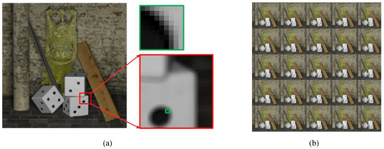
Figure 1.
Two light-field representations: (a) MI, (b) SAIs.
Although light-field imaging technology provides a wealth of information, it also poses challenges in data acquisition and processing. The Lytro Illum camera [4], for example, uses a 15 × 15 microlens array that produces high-resolution (7728 × 5368) raw LFI. The size and complexity of this raw data require efficient compression algorithms for easy storage and transmission. In addition, extracting useful visual information, such as multi-view images and depth maps, from raw light-field data requires complex processing procedures. This involves correcting optical defects such as vignetting caused by camera hardware, and optimizing image reconstruction algorithms to enhance image quality and decrease computational expenses.
In this paper, a prediction structure is proposed by analyzing the similarity of multiple views, and the reference view for each perspective is determined. The residual view is obtained by subtracting the current view from the reference view. Following this, an existing encoding scheme is introduced to achieve lossless compression by utilizing the inherent pixel distribution feature in the residual view. To further enhance compression efficiency, we concurrently apply lossy compression to the selected residual view using high-efficiency video coding (HEVC) [5]. In addition, this predictive coding scheme is designed with a hierarchical structure that enables progressive transmission.
The remainder of the paper is organized as follows: Section 2 gives an overview of methods for LFI compression; Section 3 describes the proposed prediction structure and coding schemes; in Section 4, the experimental results are presented and analyzed; finally, Section 5 summarizes the content of this article.
2. Related Work
In recent years, three main methods have been used for LFI compression: frequency domain transformation, inter-frame prediction and deep learning. Transformation-based compression techniques, such as JPEG, JPEG2000 [6], and JPEG PLENO [7], utilize frequency domain transformations like the discrete cosine transform (DCT) and discrete wavelet transform (DWT) to eliminate pixel redundancy. In the realm of DCT, Aggoun et al. [8] introduced the concept of combining images from adjacent microlens units into 3D pixel blocks and employing 3D-DCT to reduce spatial redundancy. Sgouros et al. [9] followed up by exploring different scanning methods to assemble microlens views into 3D blocks, finding superior rate-distortion performance with the Hilbert scan. More recently, Carvalho et al. [10] presented a 4D-DCT based light-field codec, MuLE, which segments the light field into 4D blocks for 4D-DCT computation, groups transform coefficients using a hexadeca-tree, and encodes the stream with an adaptive arithmetic encoder. On the DWT front, Zayed et al. [11] applied 3D-DWT to sub-aperture image stacks, recursively applying three 1D-DWTs to each dimension and producing eight subbands, followed by quantization using a dead-zone scalar quantizer and encoding with the set partitioning in hierarchical trees (SPIHT) method [12]. A comparison of two DWT-based encoding schemes (JPEG 2000 and SPIHT) against a DCT-based standard (JPEG) in terms of the reconstructed lens images’ objective quality, measured by average PSNR and SSIM indices, showed that SPIHT outperforms JPEG in RD performance, while JPEG 2000 surpasses both in terms of PSNR and SSIM [13]. However, these methods, despite their efficacy in compressing microlens-captured images, are less suitable for high-resolution multi-view images captured by multi-camera arrays. The computational complexity of DCT and DWT for high-dimensional images can be prohibitively high for real-time processing and rapid response applications. Additionally, irreversible detail distortion introduced during compression can adversely affect subsequent applications of light-field data.
Compression methods based on inter-frame prediction can be divided into pseudo-video sequence (PVS) and multi-view prediction. PVS, formed by the sub-aperture views, shows a strong correlation similar to video sequences. Thanks to the inter-frame prediction and intra-frame prediction technology of the video encoder, the video compression method can remove redundant information about the light-field data. Early efforts in this domain include Olsson et al. [14]’s utilization of the H.264 encoder to compress SAIs by assembling them into video sequences. Subsequently, Dai et al. [15] explored converting lenselet images into sub-aperture images, comparing rotary and raster scanning for compression efficiency. Vieira et al. [16] furthered this research by evaluating HEVC configurations for encoding PVS obtained from various scanning sequences, thereby advancing light-field data compression. Similarly, Hariharan et al. [17] employed HEVC to encode a similar topological scan structure. Zhao et al. [18] introduced a novel U-shaped and serpentine combined scan sequence, utilizing JEM for encoding and achieving superior results over traditional methods like JPEG. Jia et al. [19] enhanced block-based illumination compensation and adaptive filtering for reconstructed sub-aperture images, achieving notable bit savings compared to existing methods. While video encoders employing these methods achieve effective compression, they often retain the one-dimensional characteristics of video sequences. Regardless of scan order, certain views lack reference information from adjacent views, constraining the full utilization of view correlation. Multi-view prediction, however, overcomes this limitation by leveraging correlations across multiple view directions. Liu et al. [20] proposed a two-dimensional hybrid coding framework dividing the view array into seven layers with differing prediction directions. Li et al. [21] improved upon this by dividing the view array into four regions to enhance random accessibility, coupled with motion vector transformation for improved compression. Amirpour et al. also proposed an MVI structure for random accessibility, dividing the view into three layers, allowing the use of parallel processing to reduce the time complexity of multi-core codecs [22]. In addition, Ahmad et al. [23] and Zhang et al. [24] from the Central University of Sweden and Khoury’s team [25] at Columbia University regarded the SAIs as a multi-view video sequence, and proposed different prediction schemes based on the multi-view extended coding framework (MV-HEVC) of HEVC. Currently, inter-frame prediction-based schemes are predominant due to their versatility in predicting structure, offering more potential for exploiting LF correlation than direct lens image decoding.
In recent years, with the rapid development of deep learning, many models for LFI compression have been proposed. Notably, Shin et al. [26] introduced the EPINE model, leveraging convolutional neural networks (CNNs) to enhance depth estimation across the light-field array through analyses of epipolar plane images (EPIs), facilitating the reconstruction of high-quality LF images at the decoder end. Similarly, the Hedayati team’s [27] development of JPEG-Hance Net and Depth-Net, built upon JPEG, innovates in-depth map estimation from a central view, subsequently enabling the comprehensive reconstruction of the LF. This approach demonstrates marked improvements over the compression effects achieved by HEVC. Furthermore, research by Bakir et al. [28] and Jia et al. [29] explores the domain of sparse sampling of sub-aperture images (SAIs), with varied compression methodologies being devised. These methods incorporate adversarial generative networks (GANs) alongside conventional encoders, aiming to restore the full light field from both unsampled and sampled parallax perspectives. Concurrently, Yang et al. [30]’s method involves sampling images into sparse viewpoint arrays, discerning differences between adjacent microimages, and reconstructing the holistic holographic image leveraging the residual viewpoints and parallax. In a similar vein, Liu et al. [31] implemented sparse sampling of dense LF SAIs, transmitting merely the sparse SAIs and employing a multi-stream view reconstruction network (MSVRNet) at the decoder side to reconstruct the dense LF sampling area, yielding commendable outcomes.
Although these methods achieve a certain level of compression efficiency, the disadvantages and challenges they face cannot be overlooked. The inherent multi-dimensional nature of light-field images leads to a substantial volume of data, which imposes higher demands on hardware and time costs during the model training process. Furthermore, while these techniques demonstrate excellent performance on training datasets, the models’ ability to generalize across diverse scene changes remains a critical consideration.
3. Proposed Method
The multi-view prediction is utilized in designing the compression scheme because the similarity of each direction in a single view can effectively reduce redundant information. This section describes the proposed most-similar hierarchical prediction encoding (MSHPE) structure. The predictive structure of the residual view, a specific encoding order, and two specific encoding schemes will be investigated.
3.1. Proposed Prediction Structure
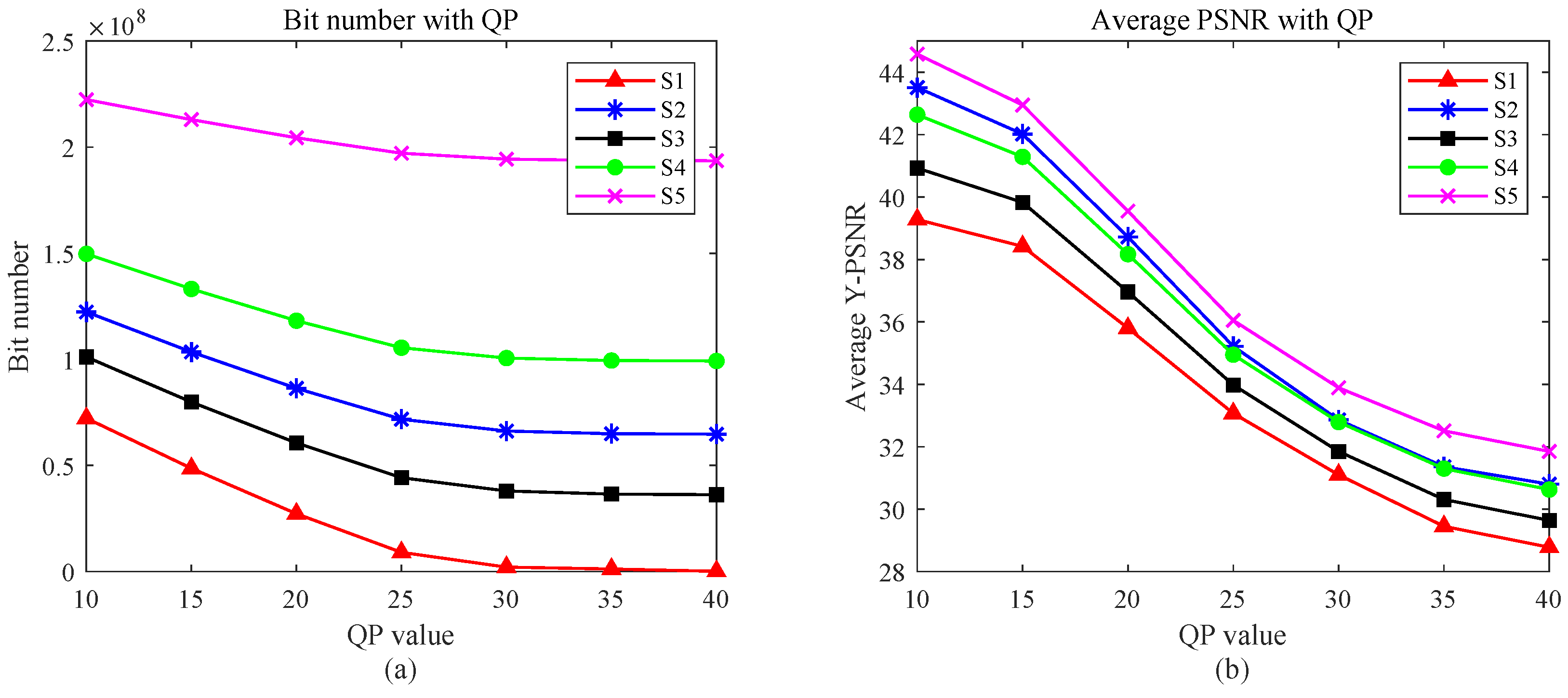
As discussed in Ref. [32], the central view presents the highest similarity with other views in the multi-view array, prompting the determination of the predictive structure initiation from the central view. However, this structure includes at most 5 × 5 views and is only applicable to light-field multi-view videos. Typically, the angular resolution of LFI reaches 9 × 9 or even 13 × 13. To further investigate the correlation between the center view and other views, a light-field dataset named HCI [33] was accessed, which contains more perspectives. It selects the “cotton” scene, calculates the average peak signal-to-noise ratio (PSNR) of the three color channels in the center view and other views, and measures the average pixel similarity of each channel. Unlike other work that utilizes the structure similarity index measure (SSIM) for measuring image similarity, PSNR was chosen because our focus was solely on pixel similarity, which aligns better with subsequent difference operations.
As illustrated in Figure 2a, the center view demonstrates the highest PSNR value with surrounding adjacent views, particularly those in the horizontal and vertical directions. Based on this observation, we perform the following operations on the views:
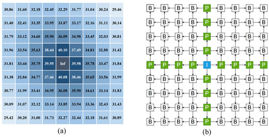
Figure 2.
(a) PSNR value between center view and other views, (b) representation of prediction structure.
Step 1: All views are divided into three groups: the central view is designated as the I-view (blue), views in the horizontal and vertical directions of the I-view form the P-view (green), and the remaining views constitute the B-view (white).
Step 2: I-view has no reference, the P-reference is the other P-views that is close to I-view in the same direction as itself, and the reference of the four P-views adjacent to the I-view is naturally I-view. In B-view, we choose two adjacent views in the direction of I-view as the pre-selection reference, but only select the one with the higher PSNR value, as shown in Figure 2b.
Step 3: After determining the reference view, the reference view is subtracted from the current view to obtain the residual array. The black arrow in Figure 2b points from the reference image to the current image.
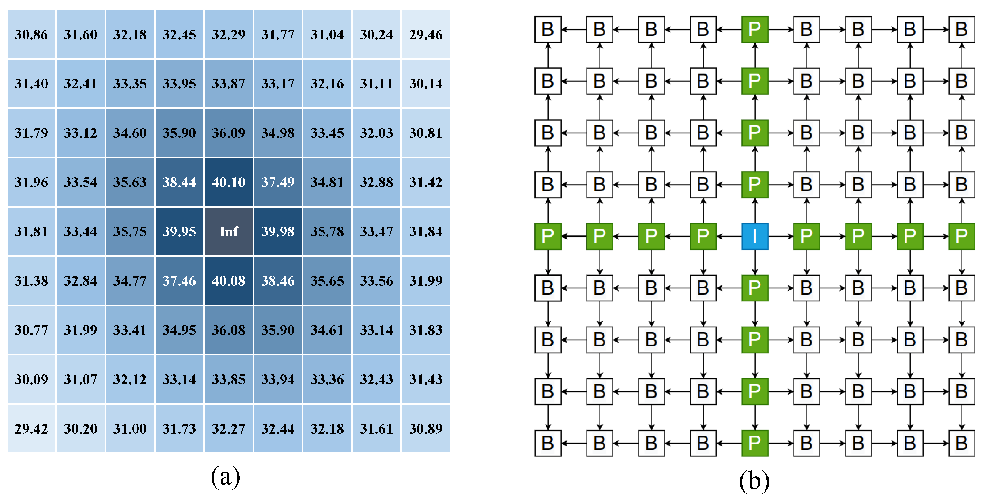
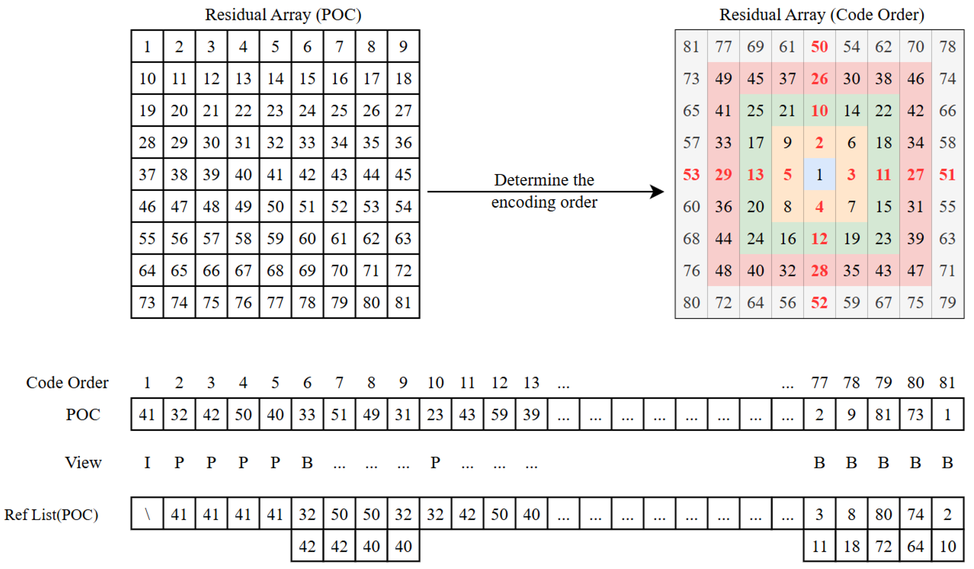
Step 4: In terms of coding order, as shown in Figure 3, the entire array is first viewed as five layers from the inside out. In each layer, four P-views are initially encoded, then one B-view in each quadrant, until all four corner B-views are encoded. For example, in the second layer, the P-views are first encoded in the order of picture order count (POC) of 32, 42, 50, 40, and then diagonally encoded in the order of POC of 33, 51, 49, 31, with only one view per quadrant at a time, and so on. The reason for this is that the current view can only be encoded after the reference view is encoded. This ensures that views from the previous layer can only be referenced during the decoding of any layer.
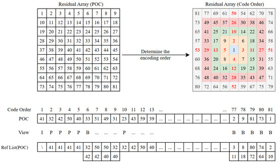
Figure 3.
Reference view and coding sequence.
The specific prediction algorithm and coding steps are also illustrated in Figure 3. The arrays are collected into a one-dimensional sequence based on the predetermined coding sequence. Subsequently, the reference list for each view is established, and the residual view is derived according to the reference list. This coding order and hierarchical structure facilitate progressive transmission in applications, both between and within layers, as elaborated upon in Section 3.3.
3.2. Encoding Scheme
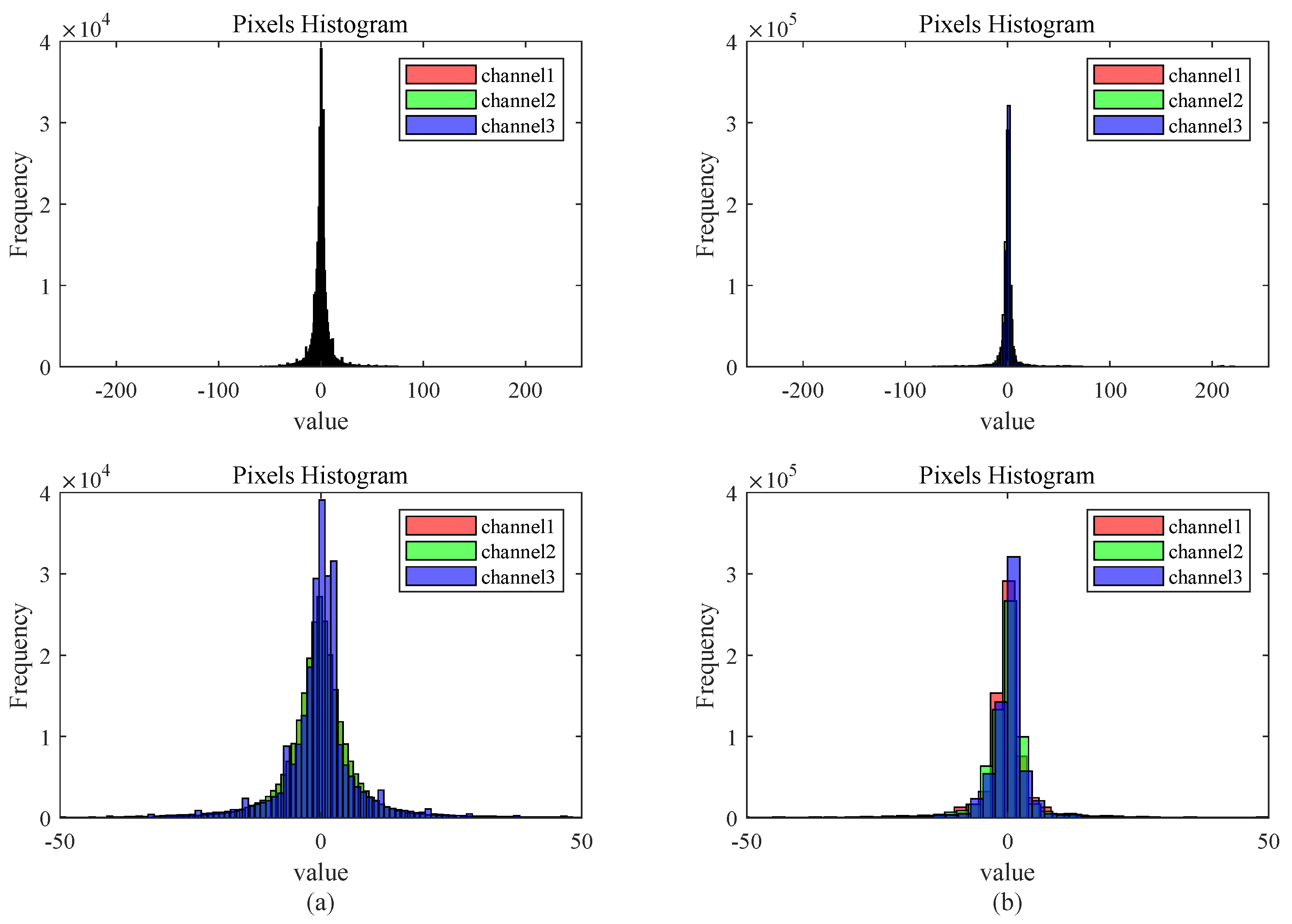
For coding residual views, this paper introduces two schemes in this paper: lossless coding and lossy coding. Using two distinct light-field scenes: “medieval” and “corner”, they come from two different LF multi-view datasets with different resolutions, including different environments, objects, light conditions, and occlusion levels. The number of pixels in the three color channels of the residual pixel matrix is calculated by applying the previously proposed prediction structure for difference processing. The resulting histogram in Figure 4 reveals that most pixel values are close to 0, with minimal occurrences near −255 or 255. In order to minimize the number of bits used, a DC coding scheme is adopted, and the specific coding principle is illustrated in Table 1. The coding process is given by Algorithm 1.
| Algorithm 1 algorithm of lossless coding. |
|
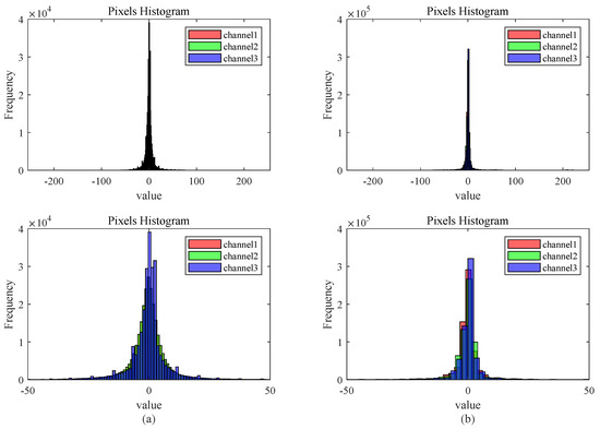
Figure 4.
Two pixel histogram of residual plots: (a) histogram of medieval’s residual, (b) histogram of corner’s residual.

Table 1.
DC coding.
This scheme divides all pixels into 9 levels, with each level using 2 to 5 bits for representation to facilitate decoding. In terms of numerical representation, high-probability pixels use short codes, and low-probability pixels use longer codes. While the latter layers have a maximum total code length of 13 for the level code, it is statistically improbable for the absolute value in the difference pixel matrix to be close to 255. After calculation, approximately 99.5% of pixel values lie in the range [−30, 30], which can greatly reduce the number of bits required to represent the pixel. So, this encoding scheme exhibits effective compression, as detailed in Section 4.1.
On the basis of the layered effect mentioned and the prevalence of smoother areas in the residual view, it was decided to use the video encoder to encode the selected partial view. This strategic choice aims to further improve the overall compression effectiveness. To prevent interference from inter-frame predictions and highlight the redundancy of individual views, the view is compressed using the full intra-frame configuration in HEVC instead of the inter-frame configuration. Specifically, all views are manipulated according to the proposed structure, each channel of the residual view is normalized to [0, 255], RGB images are synthesized, and the views are stitched together into a one-dimensional video sequence. The encoding order becomes irrelevant due to the use of a full I-frame configuration. On the decoding side, the decoded video sequence is split into individual images, converting pixels to signed integers. These are then added back to the corresponding reference view to obtain the reconstructed view.
It should be pointed out that the quality of the reconstructed views is dependent on the central view, leading to a degradation in quality with each subsequent layer. This scheme’s average image quality is not satisfactory, but it does well when it comes to bit-saving. To strike a balance between view quality and transmission cost, one can choose to employ lossless encoding for some layers and lossy encoding for others during hierarchical transmission. The detailed results of the experiments are presented in Section 4.2.
3.3. Progressive Transmission
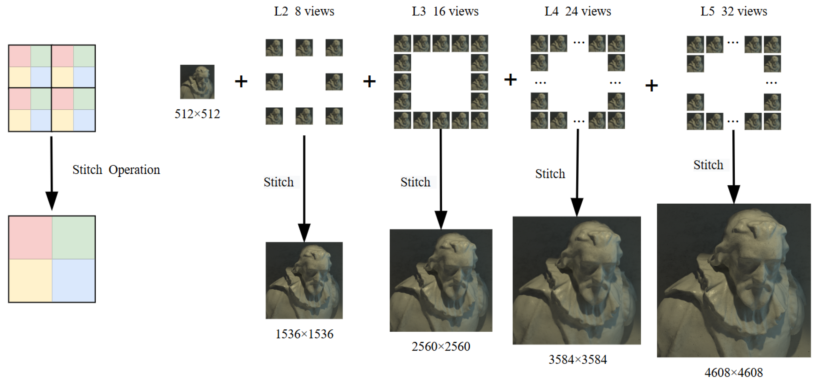
Once the coding order for all views is established, a hierarchical progressive transmission mechanism can be established. In the application of light-field data, users may sometimes require a preview of the main image information to determine whether to acquire more detailed images. Also, during transmission, limitations in network speed and hardware bandwidth resources may impede the swift transfer of substantial data to users. Hierarchical coding of views proves beneficial in such scenarios.
In the proposed scheme, the first layer is the center view, which adequately characterizes the image information. Even when using lossy encoding schemes, the center view employs lossless encoding to ensure image quality. Upon transmitting the first level of views to the user, the image information is retrieved, allowing the user to decide whether to continue receiving multi-view images. Specifically, according to Figure 3, the second layer comprises 8 views encoded from 2 to 9, the third layer consists of 16 views from 10 to 25, the fourth layer includes 24 views from 26 to 49, and the fifth layer encompasses 32 views from 50 to 81. For light-field images, previously transmitted multi-view images can be more closely approximated to the original light-field images through simple pixel stitching, parallax compensation, or super-resolution restoration technologies to cater to user needs, as shown in Figure 5.

Figure 5.
Progressive transmission diagram.
4. Experimental Results
The experimental results are presented in three parts: lossless compression, lossy compression and hierarchical progressive transfer. In the lossless segment, the compression ratios obtained by encoding the residual across different structures are compared. Meanwhile, the lossy segment evaluated the bits needed for encoding and the quality of the finally reconstructed view and compared the performance with the direct encoding of the original views using HEVC as a reference scheme. The number of lossy encoded views is then adjusted to strike a balance between compression performance and view quality. Finally, the specific data related to hierarchical progressive transmission are provided.
4.1. Lossless Compression
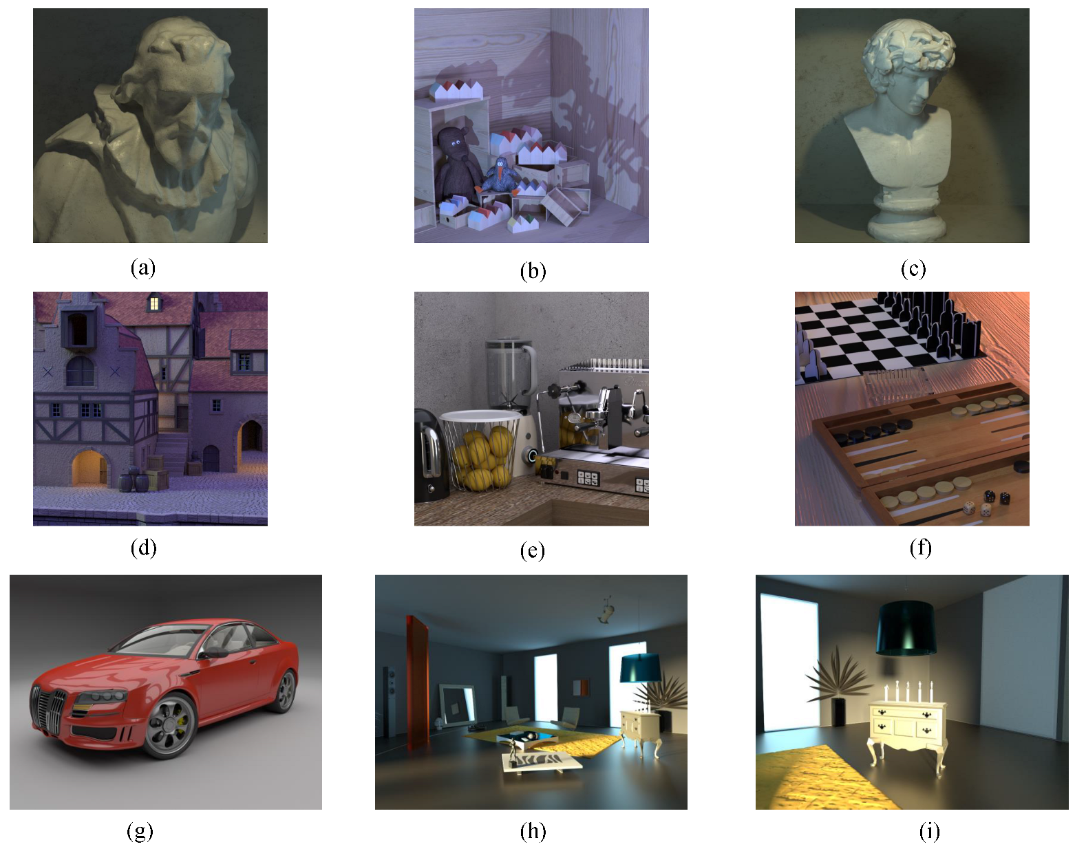
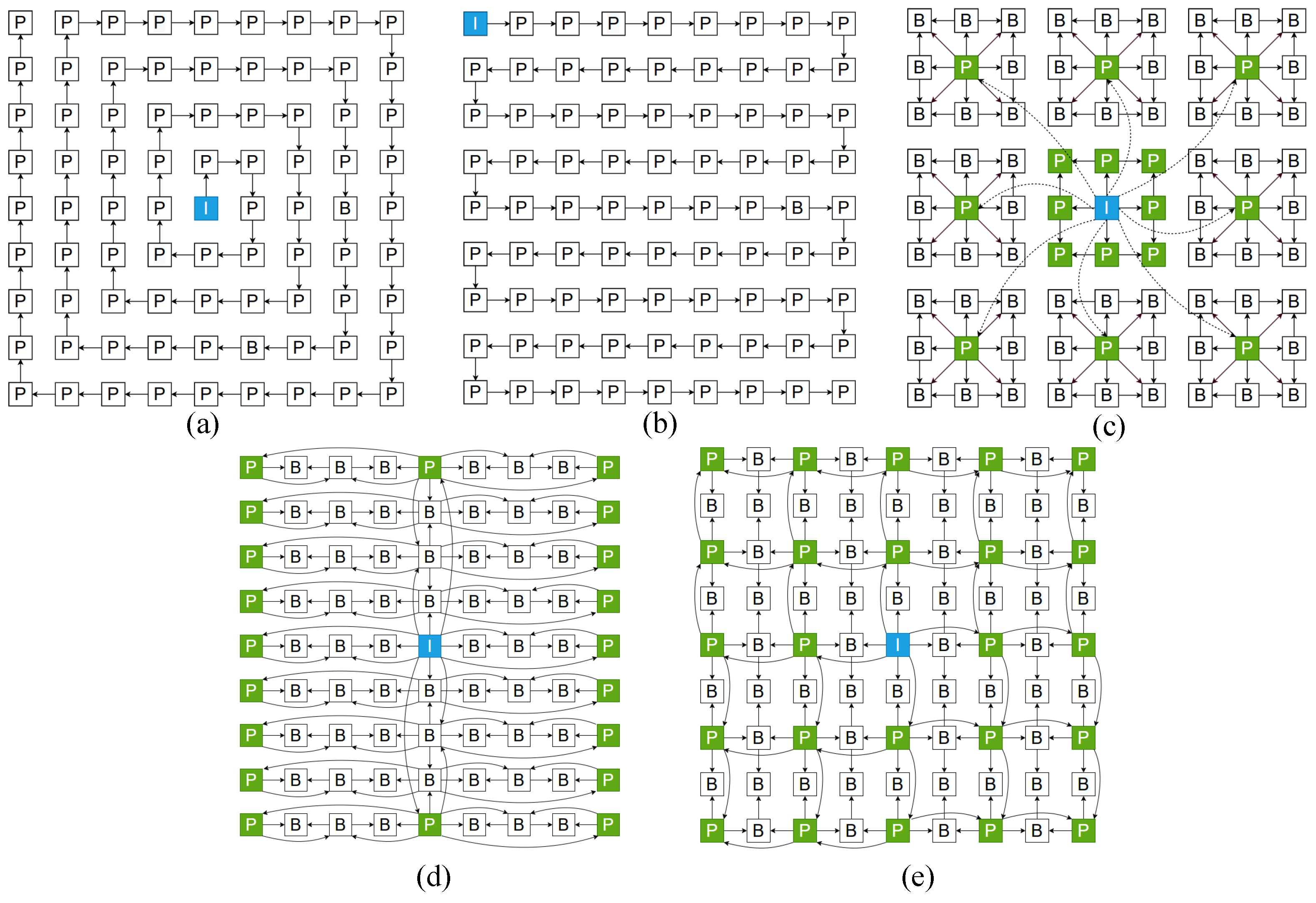
Two representative datasets, HCI and MPI [34], were chosen for the study. HCI comprises 9 × 9 views with dimensions of 512 × 512 × 3, while MPI consists of 101 views with dimensions of 960 × 720 × 3. Specifically nine center images were selected: “cotton”, “dino”, “antinous”, “medieval”, “kitchen”, “boardgames” and “car”, “room”, “corner”, the first six from HCI and the last three from MPI, as shown in Figure 6. The “medieval”, “kitchen”, “boardgames” images are used to assess the lossy compression effect. In terms of comparison structure, in addition to the spiral scanning from Ref. [35] (Figure 7a), the raster scanning from Ref. [15] (Figure 7b), MVI hierarchical structure from Ref. [22] (Figure 7c), 2-DKS in Ref. [25] (Figure 7d) and 2-DHS extracted from Ref. [21] (Figure 7e) are also included. In the original text, it is encoded as a pseudo-sequence using an encoder, but considering only conducting a difference operation on the image, we relate its structure to our approach. All views were processed according to the proposed structure.
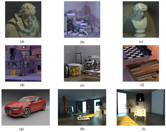
Figure 6.
The presentation of the test images. (a) Cotton, (b) dino, (c) antinous, (d) medieval, (e) kitchen, (f) boardgames, (g) car, (h) room, and (i) corner.
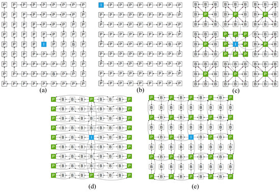
Figure 7.
The presentation of the five different prediction structures and the coding sequence and hierarchical diagram of the proposed structures. (a) Spiral, (b) raster, (c) MVI, (d) 2-DHS, (e) 2-DKS, coding order and hierarchical diagram (the different colors represent the different layers, and the numbers represent the encoding order).
For example, a one-dimensional view sequence is obtained after spiral and raster scanning, and the latter view is used to subtract the previous view. In contrast, MVI uses the center view to subtract the eight views of the second layer and then uses the eight views of the second layer to subtract the views adjacent to itself. 2-DKS and 2-DHS both use the center view as the I-view, the difference being that the former places the P-view at an interval of one frame in an odd row or column to predict the rest of the B-view, but the latter uses the middle column as the dividing line, which horizontally imitates the GOP structure in the video encoder to achieve a good prediction effect. It should be pointed out that in the figure, I-view is the beginning of the difference of the whole view, P-view is the frame with a fixed subtraction view (reference view), and B-view needs to choose a greater similarity between the two views to make the difference. Finally, the encoding scheme in Section 3.1 is applied, and the average number of bits used by three color channels of 80 views, excluding the center view, was counted. The average compression ratio C can be defined as Equation (1),
where M denotes the total number of bits used in one channel of the original image and denotes the number of bits used per channel after encoding.
The MSHPE maximizes pixel correlation in both horizontal and vertical directions, resulting in residual pixels closer to zero compared to other structures that yield larger residual values. The scheme is tested with two resolutions for scenes in the datasets (HCI: 960 × 720, 480 × 360, MPI: 512 × 512, 128 × 128). The number of encoded bits required is fewer, and the compression ratio is higher, as indicated in Table 2. Further, Table 3 also gives the differences in the compression ratio of other people’s methods relative to the methods in this paper.
Table 2.
Comparison of compression ratios (the experiment used six scene images from two datasets).
Table 3.
Compression ratio difference of others with respect to MSHPE.
A comparison with the reference list of the proposed scheme against the spiral scan order reveals that our scheme consistently selects the most similar neighbors for difference, while the raster scan may cause some views to choose dissimilar ones, leading to larger residual values. On the other hand, MVI, 2-DKS, and 2-DHS limit the use of similarity by choosing a P-view that is farther away when they first use the I-view to make a difference.
Furthermore, the random accessibility of the view is a crucial aspect of the coding structure. Random accessibility pertains to the attributes of a particular view requiring decoding, typically influenced by the number of preceding views that must be decoded. MVI is specially designed for random accessibility, and only three views need to be decoded. For 2-DKS and 2-DHS, five views need to be decoded in the worst case. With spiral scanning and raster scanning, the effectiveness of random accessibility decreases as the view scan order increases, possibly requiring decoding the entire view set in the worst case. Our proposed scheme’s random accessibility is tied to the prediction relationship rather than the coding order. The number of decoded views needed to decode any view from the first to the fifth layer is 0, 2, 4, 6, and 8, respectively. This feature ensures that our choice of the center view as the first layer is justified to a certain extent.
4.2. Lossy Compression
In order to prove the superiority of the MSHPE and to further improve the compression ratio, the remaining views except the center view are lossy encoded. The HEVC reference encoder software HM16.20 [36] is used in our evaluation. To exclude interference from inter-frame prediction, only the full intra-frame configuration is used.
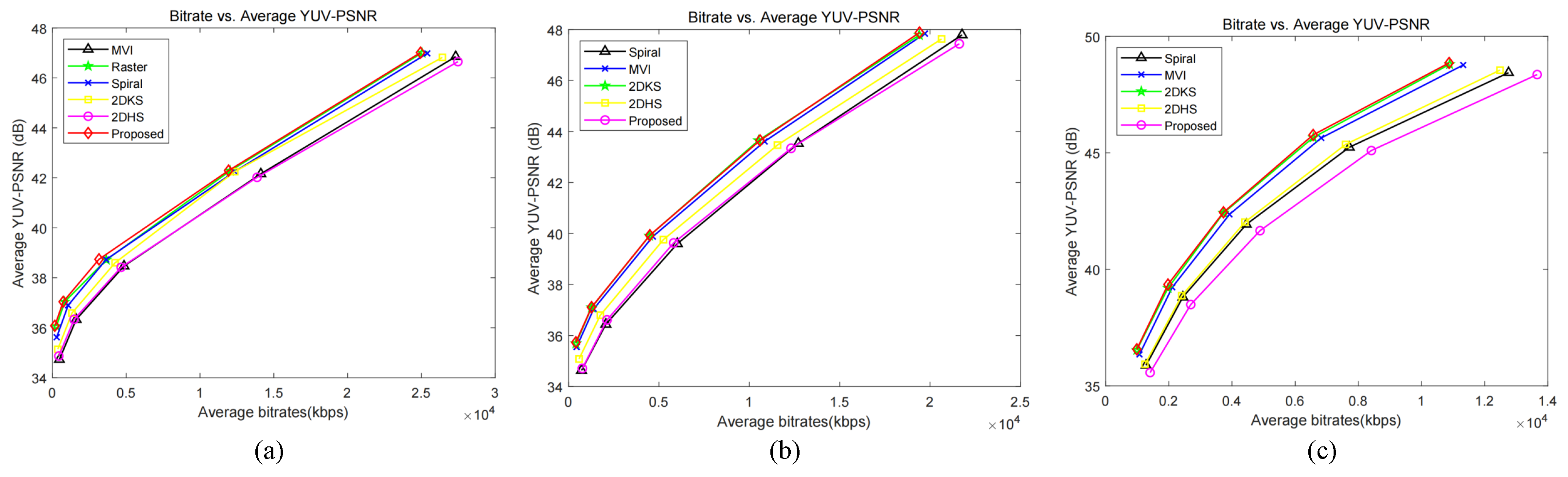
According to the suggestions and structure of Figure 6a–e, differences in each channel of the “medieval”, “kitchen”, and “boardgame” views were initially preprocessed. Then, the difference between the three channels is combined to form several difference views, and the video sequence required for HEVC is synthesized (Y:U:V = 4:2:0). Specifically, we take QP = 17, 22, 27, 32, 37 and encode the three difference sequences separately, and the final result is shown in Figure 7. In HEVC, the QP value is a quantization parameter that determines the bitrate. From the perspective of the rate-of-distortion curve, the processed image in this paper has better bit-saving performance and has better quality gain at both lower and higher bitrates (Figure 8).
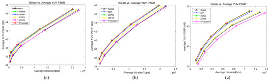
Figure 8.
Rate-of-distortion curves for different difference sequences were encoded using HEVC: (a) medieval, (b) kitchen, (c) boardgames.
In addition, it is important to recognize that coding residuals have a detrimental effect on the quality of the final reconstructed image. The decoded residual sequence sub-channel can be added to the corresponding reference image to obtain the reconstructed image, but due to the large loss of information in the residuals, the objective quality of the reconstructed view is not as good as that of the view directly recovered by HEVC encoding, as shown in Table 4. According to our calculations: BD-BR = −68.67% and BD-PSNR = −2.74 dB. That is, at the same bitrate, the quality of the reconstructed view after encoding residuals decreases by an average of 2.74 dB, but the direct encoded view requires an average of 68.67% more bits to achieve the same quality as the latter. This is enough to prove the superiority of the residual coding method in this paper in terms of bit-saving.
Table 4.
The bitrate (kbps) and the average Y-PSNR (dB) by HEVC and MSHPE.
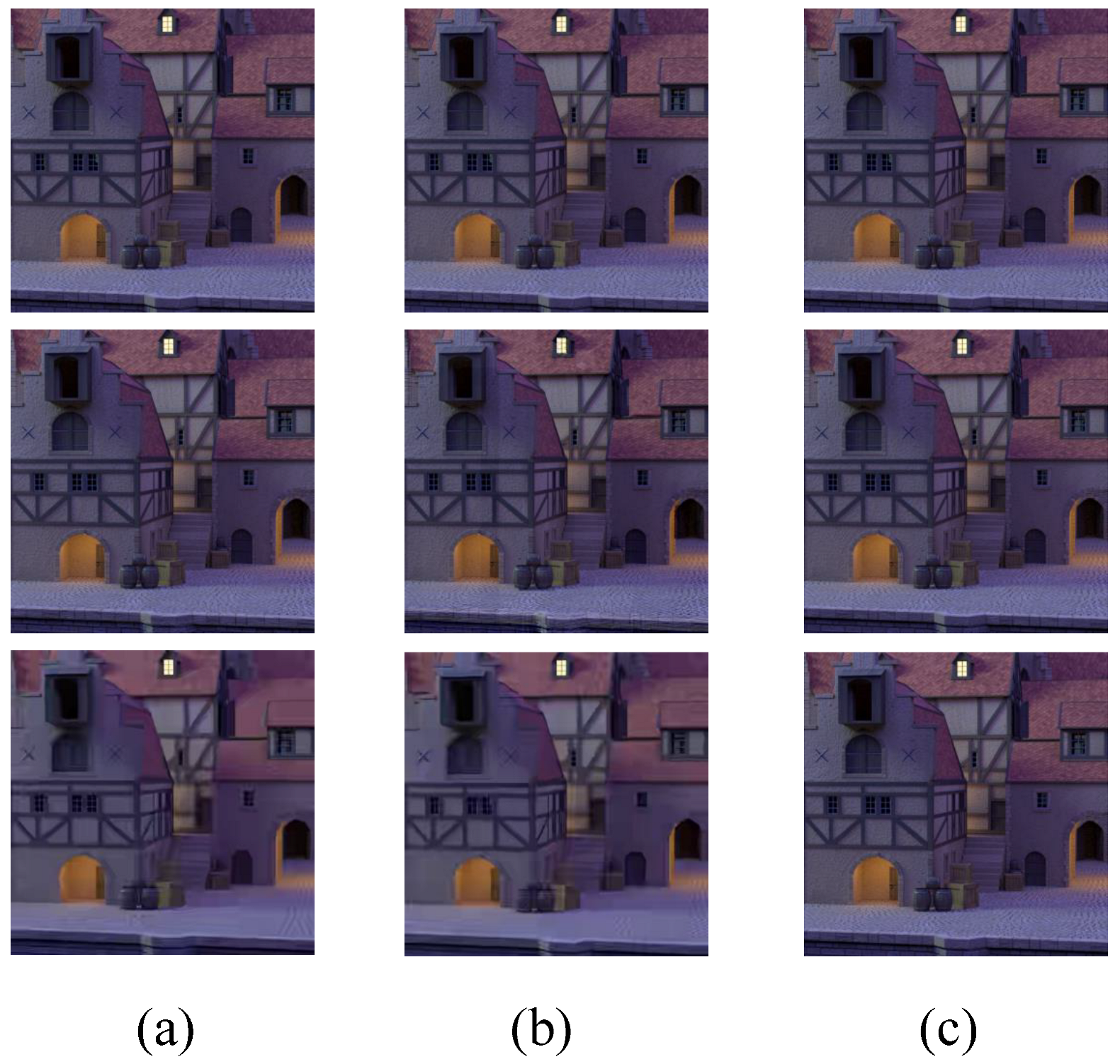
Specifically, in the comparison of subjective quality, the views encoded with HEVC exhibited significant visual distortion. As shown in Figure 9a,c, the proposed scheme is significantly better than HEVC in recovering image details when QP = 40, and almost the same when QP = 20. In addition, after comparing Figure 9a,b, the reconstructed view of layer 5 with coordinates (1, 1) is not as detailed as the reconstructed view of layer 2 with coordinates (4, 5), although it is not as detailed as the reconstructed view of HEVC. This result highlights the feasibility of encoding residuals, further supporting the superiority of our method in terms of bit savings and maintaining image fidelity.
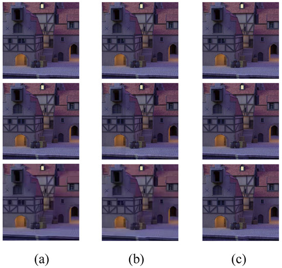
Figure 9.
Comparison of the details of the original image and the reconstruction images after MSHPE and HEVC. (a) QP = 40, location is (4,5) (b) QP = 40, location is (1,1), (c) QP = 20, location is (4,5).
Moreover, in lossy encoding, the selection of views from various layers significantly influences both the consumed bit count and the final reconstructed view quality. This paper establishes five comparison schemes, denoted as , guided by the hierarchical framework outlined in Section 3.3. These schemes encompass lossy encoding for all views except I-view (), encoding for views excluding I-view and P-view (), lossy encoding solely for layers 3, 4, and 5 (), exclusive lossy encoding for layers 4 and 5 (), and exclusive lossy encoding for layer 5 (). Subsequently, Figure 10 shows the bit consumption for each scenario and the average quality of the recovered view. Obviously, yields the highest image quality; However, the associated bit count renders it impractical. On the other hand, and exhibit lower bit requirements but achieve diminished image quality. Striking an optimal balance between bit count and view quality entails a choice between and . Both schemes demonstrate nearly identical quality curves, with requiring fewer bits, making it a judicious choice for achieving a balance between bit count and reconstructed view quality.
4.3. Computational Complexity Analysis
The determination of the reference list involves only the assignment and initialization of variables, so it is a constant-time operation. Image traversal and rearrangement: This step involves two nested loops that traverse the rows and columns of the image, respectively. For an image, the time complexity of this step is O (). Since there are 81 such matrices, the total time complexity is O (). Conversion to one-dimensional sequence difference processing: This step involves another nested loop to convert a 2D matrix into a one-dimensional sequence. For an matrix, the time complexity of this operation is O (). Since there are 81 such matrices, the total time complexity is O (). Difference processing also involves traversing these matrices, so it has the same time complexity. Encoding: The encoding step involves encoding each pixel, which is usually a constant-time operation. For an matrix, the time complexity of the encoding is O (). Since there are 81 such matrices, the total time complexity is O (). To sum up, the time complexity of this function mainly depends on the size and number of images and can be expressed as O (), where M and N represent the number of rows and columns of the image, respectively.
4.4. Progressive Transmission
As mentioned above, the proposed coding structure offers adaptability for progressive transmission to cater to diverse transmission requirements. Building upon the scheme in Section 4.2, we explored progressive transmission. Starting with the central view and incrementally adding one layer at a time until all views are transmitted, Table 5 details the bitrate for each transfer and the average quality of the transmitted views. Notably, regardless of the chosen quantization value, the average quality of the reconstructed view diminishes with each additional layer.
Table 5.
Average Y-PSNR (dB) and bit rate (kbps) for progressive transmission at different quantization values.
This decline is due to the fact that in our structure, the view of the previous layer is always used as a reference for the view of the next layer, so when the quality of the previous layer is affected, the quality of the subsequent layers is also affected, and the outermost view is affected the most. In practical usage, this transmission system exclusively transmits light-field data that meet the needs of users. For example, sometimes, the user needs to obtain the information of the image in a short time, but it takes time to transmit the complete data, so first, we transmit part of the layer; at this time, the image resolution is very low, and then through the supplementation of more layers, the resolution of the image increases. It has the ability to reduce redundant data, improve network bandwidth utilization, and enhance system response speed and performance simultaneously.
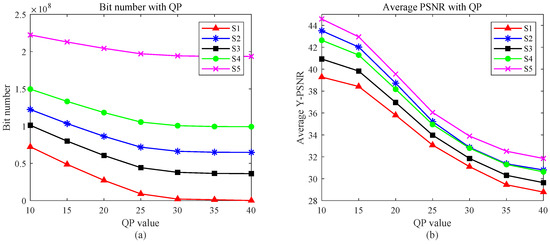
Figure 10.
Graphs of the number of bits and the average Y-PSNR as a function of QP for the five schemes: (a) curve of number of bits with QP, (b) curve of average Y-PSNR with QP.
Figure 10.
Graphs of the number of bits and the average Y-PSNR as a function of QP for the five schemes: (a) curve of number of bits with QP, (b) curve of average Y-PSNR with QP.
5. Conclusions
This paper proposes a new two-dimensional prediction structure based on the similarity between light-field multi-view images, which divides the views into three categories. Different categories of views have different prediction rules. After the reference view is determined, the entire array is divided into four quadrants considering random access, and the final coding order is determined based on the sequential coding of the quadrants. Based on the obtained residual view array, a coding method is proposed to perform lossless coding of the residual view. Experimental results show that the compression rate of this prediction method is higher. When using HEVC to perform lossy encoding and decoding of the residual, the experimental results show that a certain amount of bits can be saved. Although the quality of the final restored view is slightly lower, it is still within the acceptable range, and the details of the image are visually better than the former. At the same time, this encoding structure can also implement progressive transmission functions to meet the needs of different scenarios. In lossy progressive transmission, as long as the quality of the first few layers close to the center view is good enough, a better quality view can be presented to the user, while the views in the outer layers only play a role in supplementing image detail information.
Author Contributions
Conceptualization, J.S. and E.B.; methodology, J.S. and E.B.; software, J.S.; validation, J.S.; formal analysis, J.S. and E.B.; investigation, J.S.; resources, E.B. and X.J.; data curation, X.J.; writing—original draft preparation, J.S.; writing—review and editing, E.B., X.J. and Y.W.; visualization, J.S.; supervision, E.B., X.J. and Y.W.; project administration, E.B.; funding acquisition, E.B. All authors have read and agreed to the published version of the manuscript.
Funding
This work was supported in part by the National Natural Science Foundation of Shanghai under Grant 20ZR1400700 and the National Natural Science Foundation of China under Grant 61972080.
Institutional Review Board Statement
Not applicable.
Informed Consent Statement
Not applicable.
Data Availability Statement
The data are not publicly available due to privacy and can be obtained upon reasonable request.
Conflicts of Interest
The authors declare no conflicts of interest.
References
- Landy, M.; Movshon, J.A. The Plenoptic Function and the Elements of Early Vision. In Computational Models of Visual Processing; MIT Press: Cambridge, CA, USA, 1991; pp. 3–20. [Google Scholar]
- Levoy, M.; Hanrahan, P. Light field rendering. In Proceedings of the 23rd annual conference on Computer Graphics and Interactive Techniques, New Orleans, LA, USA, 4–9 August 1996; pp. 31–42. [Google Scholar]
- Ye, K.; Li, Y.; Li, G.; Jin, D.; Zhao, B. End-to-End Light Field Image Compression with Multi-Domain Feature Learning. Appl. Sci. 2024, 14, 2271. [Google Scholar] [CrossRef]
- Ng, R.; Levoy, M.; Brédif, M.; Duval, G.; Horowitz, M.; Hanrahan, P. Light Field Photography with a Hand-Held Plenoptic Camera. Doctoral Dissertation, Stanford University, Stanford, CA, USA, 2005. [Google Scholar]
- Sullivan, G.J.; Ohm, J.R.; Han, W.J.; Wiegand, T. Overview of the high efficiency video coding (HEVC) standard. IEEE Trans. Circuits Syst. Video Technol. 2012, 22, 1649–1668. [Google Scholar] [CrossRef]
- Skodras, A.; Christopoulos, C.; Ebrahimi, T. The JPEG 2000 still image compression standard. IEEE Signal Process. Mag. 2001, 18, 36–58. [Google Scholar] [CrossRef]
- Bach, N.G.; Tran, C.M.; Duc, T.N.; Tan, P.X.; Kamioka, E. Novel Projection Schemes for Graph-Based Light Field Coding. Sensors 2022, 22, 4948. [Google Scholar] [CrossRef] [PubMed]
- Aggoun, A. A 3D DCT compression algorithm for omnidirectional integral images. In Proceedings of the IEEE International Conference on Acoustics Speech and Signal Processing, Toulouse, France, 14–19 May 2006. [Google Scholar]
- Sgouros, N.; Kontaxakis, I.; Sangriotis, M. Effect of different traversal schemes in integral image coding. Appl. Opt. 2008, 47, D28–D37. [Google Scholar] [CrossRef] [PubMed]
- Carvalho, M.B.; Pereira, M.P.; Alves, G.; da Silva, E.A.; Pagliari, C.L.; Pereira, F.; Testoni, V. A 4D DCT-Based Lenslet Light Field Codec. In Proceedings of the IEEE International Conference on Image Processing (ICIP), Athens, Greece, 7–10 October 2018; pp. 435–439. [Google Scholar]
- Zayed, H.H.; Kishk, S.E.; Ahmed, H.M. 3D wavelets with SPIHT coding for integral imaging compression. Int. J. Comput. Sci. Netw. Secur. 2012, 12, 126–133. [Google Scholar]
- Said, A.; Pearlman, W.A. A new, fast, and efficient image codec based on set partitioning in hierarchical trees. IEEE Trans. Circuits Syst. Video Technol. 1996, 6, 243–250. [Google Scholar] [CrossRef]
- Higa, R.S.; Chavez, R.F.L.; Leite, R.B.; Arthur, R.; Iano, Y. Plenoptic image compression comparison between JPEG, JPEG2000 and SPITH. Cyber J. JSAT 2013, 3, 1–6. [Google Scholar]
- Olsson, R.; Sjostrom, M.; Xu, Y. A combined pre-processing and H. 264-compression scheme for 3D integral images. In Proceedings of the International Conference on Image Processing, Atlanta, GA, USA, 8–11 October 2006; pp. 513–516. [Google Scholar]
- Dai, F.; Zhang, J.; Ma, Y.; Zhang, Y. Lenselet image compression scheme based on subaperture images streaming. In Proceedings of the IEEE International Conference on Image Processing (ICIP), Quebec City, QC, Canada, 27–30 September 2015; pp. 4733–4737. [Google Scholar]
- Vieira, A.; Duarte, H.; Perra, C.; Tavora, L.; Assuncao, P. Data formats for high efficiency coding of Lytro-Illum light fields. In Proceedings of the International Conference on Image Processing Theory, Tools and Applications (IPTA), Orleans, France, 10–13 November 2015; pp. 494–497. [Google Scholar]
- Hariharan, H.P.; Lange, T.; Herfet, T. Low complexity light field compression based on pseudo-temporal circular sequencing. In Proceedings of the IEEE International Symposium on Broadband Multimedia Systems and Broadcasting (BMSB), Cagliari, Italy, 7–9 June 2017; pp. 1–5. [Google Scholar]
- Zhao, S.; Chen, Z.; Yang, K.; Huang, H. Light field image coding with hybrid scan order. In Proceedings of the Visual Communications and Image Processing (VCIP), Chengdu, China, 27–30 November 2016; pp. 1–4. [Google Scholar]
- Jia, C.; Yang, Y.; Zhang, X.; Zhang, X.; Wang, S.; Wang, S.; Ma, S. Optimized interview prediction based light field image compression with adaptive reconstruction. In Proceedings of the IEEE International Conference on Image Processing (ICIP), Beijing, China, 17–20 September 2017; pp. 4572–4576. [Google Scholar]
- Liu, D.; Wang, L.; Li, L.; Xiong, Z.; Wu, F.; Zeng, W. Pseudo-sequence-based light field image compression. In Proceedings of the IEEE International Conference on Multimedia & Expo Workshops (ICMEW), Seattle, WA, USA, 11–15 July 2016; pp. 1–4. [Google Scholar]
- Li, L.; Li, Z.; Li, B.; Liu, D.; Li, H. Pseudo-sequence-based 2-D hierarchical coding structure for light-field image compression. IEEE J. Sel. Top. Signal Process. 2017, 11, 1107–1119. [Google Scholar] [CrossRef]
- Amirpour, H.; Pinheiro, A.; Pereira, M.; Lopes, F.J.; Ghanbari, M. Efficient light field image compression with enhanced random access. ACM Trans. Multimedia Comput. Commun. Appl. 2022, 18, 1–18. [Google Scholar] [CrossRef]
- Ahmad, W.; Olsson, R.; Sjöström, M. Interpreting plenoptic images as multi-view sequences for improved compression. In Proceedings of the IEEE International Conference on Image Processing (ICIP), Beijing, China, 17–20 September 2017; pp. 4557–4561. [Google Scholar]
- Zhang, X.; Wang, H.; Tian, T. Light field image coding with disparity correlation based prediction. In Proceedings of the IEEE Fourth International Conference on Multimedia Big Data (BigMM), Xi’an, China, 13–16 September 2018; pp. 1–6. [Google Scholar]
- Khoury, J.; Pourazad, M.T.; Nasiopoulos, P. A new prediction structure for efficient MV-HEVC based light field video compression. In Proceedings of the International Conference on Computing, Networking and Communications (ICNC), Honolulu, HI, USA, 18–21 February 2019; pp. 588–591. [Google Scholar]
- Shin, C.; Jeon, H.G.; Yoon, Y.; Kweon, I.S.; Kim, S.J. Epinet: A fully convolutional neural network using epipolar geometry for depth from light field images. In Proceedings of the IEEE Conference on Computer Vision and Pattern Recognition (CVPR), Salt Lake City, UT, USA, 18–23 June 2018; pp. 4748–4757. [Google Scholar]
- Hedayati, E.; Havens, T.C.; Bos, J.P. Light field compression by residual CNN-assisted JPEG. In Proceedings of the International Joint Conference on Neural Networks (IJCNN), Shenzhen, China, 18–22 July 2021; pp. 1–9. [Google Scholar]
- Bakir, N.; Hamidouche, W.; Fezza, S.A.; Samrouth, K.; Deforges, O. Light field image coding using VVC standard and view synthesis based on dual discriminator GAN. IEEE Trans. Multimed. 2021, 23, 2972–2985. [Google Scholar] [CrossRef]
- Jia, C.; Zhang, X.; Wang, S.; Wang, S.; Ma, S. Light field image compression using generative adversarial network-based view synthesis. IEEE J. Emerg. Sel. Top. Circuits Syst. 2018, 9, 177–189. [Google Scholar] [CrossRef]
- Yang, L.; An, P.; Liu, D.; Ma, R.; Shen, L. Three-dimensional holoscopic image-coding scheme using a sparse viewpoint image array and disparities. J. Electron. Imaging 2018, 27, 033030. [Google Scholar] [CrossRef]
- Liu, D.; Huang, Y.; Fang, Y.; Zuo, Y.; An, P. Multi-stream dense view reconstruction network for light field image compression. IEEE Trans. Multimed. 2022, 25, 4400–4414. [Google Scholar] [CrossRef]
- Mehajabin, N.; Pourazad, M.T.; Nasiopoulos, P. An efficient pseudo-sequence-based light field video coding utilizing view similarities for prediction structure. IEEE Trans. Circuits Syst. Video Technol. 2021, 32, 2356–2370. [Google Scholar] [CrossRef]
- Honauer, K.; Johannsen, O.; Kondermann, D.; Goldluecke, B. A dataset and evaluation methodology for depth estimation on 4D light fields. In Proceedings of the Computer Vision—ACCV 2016: 13th Asian Conference on Computer Vision, Taipei, Taiwan, 20–24 November 2016; pp. 19–34. [Google Scholar]
- Kiran, A.V.; Vinkler, M.; Sumin, D.; Mantiuk, R.K.; Myszkowski, K.; Seidel, H.P.; Didyk, P. Towards a quality metric for dense light fields. In Proceedings of the IEEE Conference on Computer Vision and Pattern Recognition (CVPR), Honolulu, HI, USA, 21–26 July 2017; pp. 58–67. [Google Scholar]
- Rizkallah, M.; Maugey, T.; Yaacoub, C.; Guillemot, C. Impact of light field compression on focus stack and extended focus images. In Proceedings of the European Signal Processing Conference (EUSIPCO), Budapest, Hungary, 29 August–2 September 2016; pp. 898–902. [Google Scholar]
- High Efficiency Video Coding Test Model, HM-16.20. Available online: https://hevc.hhi.fraunhofer.de/svn/svn_HEVCSoftware/tags/HM-16.20/ (accessed on 5 May 2024).

Disclaimer/Publisher’s Note: The statements, opinions and data contained in all publications are solely those of the individual author(s) and contributor(s) and not of MDPI and/or the editor(s). MDPI and/or the editor(s) disclaim responsibility for any injury to people or property resulting from any ideas, methods, instructions or products referred to in the content. |
© 2024 by the authors. Licensee MDPI, Basel, Switzerland. This article is an open access article distributed under the terms and conditions of the Creative Commons Attribution (CC BY) license (https://creativecommons.org/licenses/by/4.0/).