Abstract
Channel estimation accuracy significantly affects the performance of orthogonal frequency-division multiplexing (OFDM) systems. In the literature, there are quite a few channel estimation methods. However, the performances of these methods deteriorate considerably when the wireless channels suffer from nonlinear distortions and interferences. Machine learning (ML) shows great potential for solving nonparametric problems. This paper proposes ML-based channel estimation methods for systems with comb-type pilot patterns and random pilot symbols, such as ATSC 3.0. We compare their performances with conventional channel estimations in ATSC 3.0 systems for linear and nonlinear channel models. We also evaluate the robustness of the ML-based methods against channel model mismatch and signal-to-noise ratio (SNR) mismatch. The results show that the ML-based channel estimations achieve good mean squared error (MSE) performance for linear and nonlinear channels if the channel statistics used for the training stage match those of the deployment stage. Otherwise, the ML estimation models may overfit the training channel, leading to poor deployment performance. Furthermore, the deep neural network (DNN)-based method does not outperform the linear channel estimation methods in nonlinear channels.
1. Introduction
The Advanced Television Systems Committee (ATSC) standardized its next-generation digital terrestrial television standard, ATSC 3.0, in 2016 [1]. This new standard brings several improvements over the previous ATSC 1.0 standard, including more channels, better video quality, mobile television, on-demand internet content, and more. One of the main reasons that ATSC 3.0 achieves these improvements is the utilization of the orthogonal frequency-division multiplexing (OFDM) technique, which is well known for its high spectral efficiency and ability to cope with frequency-selective fading. In a wireless communication channel, the transmitted OFDM signals are usually distorted by multipath fading, which differs on different subcarriers. The transmitted information can only be correctly recovered if the receiver can accurately estimate the fading at each subcarrier. Thus, channel estimation accuracy significantly affects the performance of OFDM systems. Transmission resources, referred to as pilots, are reserved and utilized to facilitate channel estimation in most OFDM systems. ATSC 3.0 employs a comb-type pilot arrangement for the purpose.
Much literature exists on pilot-based channel estimation in OFDM systems [2,3,4]. The conventional channel estimation methods proposed can be roughly divided into the following categories: linear minimum mean square error (LMMSE) method [5], functional interpolation [6,7], discrete Fourier transform-based (DFT-based) approach [8,9], and decision-directed approach [10,11]. However, these methods are computationally intensive, hard to implement, or perform poorly.
Machine learning (ML) has recently attracted attention in wireless communications [12,13,14,15]. Unlike the conventional design, which depends on mathematically expressed models, ML is a model-free and data-driven method, thus showing great potential for solving nonparametric problems. Moreover, parallel architecture could execute the learned algorithms faster and with lower power consumption. Over the last few years, several papers on ML-based channel estimation methods have been published. However, no research exists evaluating the potential of applying ML-based channel estimation methods at data subcarriers for systems with comb-type pilot patterns and random pilot symbols, such as ATSC 3.0 systems.
The contributions of this paper are summarized as follows:
- We propose an ML approach to estimate channel frequency responses (CFRs) for systems with comb-type pilot patterns and random pilot symbols, such as ATSC 3.0 systems. This paper introduces the support vector regression (SVR) [16] and deep neural network (DNN) [17] estimation methods, in which the least squares (LS) estimates of the pilot and pseudo-pilot CFRs are fed into the ML models to generate enhanced CFR estimates for data subcarriers.
- We find the number of pilots achieving good cost-effectiveness. In [18], it is observed that the more pilots used in estimation, the more accurate the estimation results are, but at the cost of increased computational complexity. However, channel estimation is performed on television sets, which are edge computing devices with limited computational resources. Therefore, our contribution lies in finding the most cost-effective numbers of pilots to use in ML models that are close to but have yet to pass the point of diminished return.
- We comprehensively evaluate the ML approach using various ML methods, including the linear SVR, SVR with radical-basis-function (RBF) kernel, and DNN. Furthermore, we compare the performances of these ML methods with those of conventional channel estimation methods, such as LMMSE- and DFT-based channel estimation methods, in both linear and nonlinear channel models. Additionally, we assess the robustness of the ML-based methods against delay profile mismatch and signal-to-noise ratio (SNR) mismatch, ensuring a thorough and reliable evaluation process.
- We find that DNN cannot improve the performances of SVR and LMMSE for both linear and nonlinear channel models. Refs. [19,20] observed that DNN has great potential in combatting nonlinear distortion and is thus a preferred choice for nonlinear channels. However, this observation does not hold in our simulation results. Although it is a negative result, our contribution is that we demonstrate that DNN may not be the answer to all nonlinear channels and systems. We show its limitations.
Finally, we observe that although the performances of the channel estimation methods are evaluated in ATSC 3.0 systems, the results obtained in this paper provide a reference model for most single-input single-output (SISO) OFDM systems since most OFDM systems have similar designs and pilot patterns.
The outline of the paper is as follows. Section 2 briefly reviews related work on different approaches to the channel estimation problem. The pilot pattern in ATSC 3.0 and the training data for ML-based channel estimation methods are described in Section 3. Section 4 presents the ML-based and conventional channel estimation methods compared in this paper. In Section 5 and Section 6, the performances of the channel estimation methods are compared in linear and nonlinear channel models, respectively. Section 7 discusses the limitations of the proposed methods. Finally, conclusions are drawn in Section 8.
2. Background and Related Work
The conventional channel estimation methods can be roughly divided into the following categories: LMMSE method, functional interpolation, DFT-based approach, and decision-directed approach. LMMSE is the optimal estimation technique if the channel is linear [5]. However, LMMSE suffers from three main impediments which limit its practical application. Firstly, it is computationally intensive since LMMSE involves a matrix inversion and multiple matrix multiplications. Secondly, its implementation requires the receiver’s prior knowledge of second-order statistics about the channel and noise, which are unavailable in most practical systems. Third, the performance of LMMSE degrades significantly if the channel is nonlinear.
In functional interpolation methods [6,7], the channel frequency response at a data subcarrier is obtained using interpolation techniques, such as linear and cubic, based on the CFR estimates at neighboring pilots. The functional interpolation methods are categorized into two categories. One-dimensional (1D) estimation independently employs interpolation techniques across subcarriers in each OFDM symbol, while two-dimensional (2D) estimation employs interpolation techniques across both OFDM symbol and subcarriers. These methods are easy to implement and are independent of accurate channel statistics. However, their performances are significantly inferior to all the other methods considered in this paper, especially for small SNR values.
The DFT-based approach [8,9] can be divided into two subcategories: interpolation [21] and smoothing [22]. In the DFT-based interpolation approach, only pilot CFRs are fed into the DFT-based estimation module, and the CFRs at data subcarriers are estimated. In the DFT-based smoothing approach, a simple interpolation scheme, e.g., 1D or 2D, is used first to obtain the CFRs at data subcarriers based on pilot CFRs. Then, the estimation module refines the CFR estimates at pilot and data subcarriers using DFT smoothing for noise reduction. In this paper, we consider the DFT-based interpolation approach as it is a more popular method. DFT-based interpolation employs inverse DFT (IDFT) to transform pilot CFR estimates in an OFDM symbol into the samples of channel impulse response (in the time domain). A time window then truncates the sample sequence to remove as much noise as possible while keeping all significant parts of channel impulse response intact. Finally, the truncated sample sequence is fast Fourier transformed to obtain the interpolated CFRs at data subcarriers after being zero-padded to the entire length of the OFDM symbol. Although the method can perform well, finding a proper truncation window length is difficult.
The decision-directed approach [10,11] is an iterative method that employs corrected data bits to refine the CFR estimates. Firstly, the receiver employs a simple channel estimation method to acquire the initial estimates. The data bits are obtained after demodulation and decoding and then re-encoded and remodulated to obtain the estimated transmitted symbol at all data subcarriers. Thus, the receiver can re-estimate the CFRs again using all subcarriers as pilots. The whole process may be repeated several times to improve estimation accuracy. This approach can produce better channel estimates but at the cost of extra computationally intensive encoding and decoding processes.
Over the last few years, several papers on ML-based channel estimation methods have been published. Refs. [18,19] theoretically analyze the performances of ML-based methods. In [18], an upper bound of the mean squared error (MSE) difference between minimum mean square error (MMSE) and ML-based channel estimations is derived for linear channels, providing theoretical support for the ML-based channel estimation. Moreover, it is proved that the MSE difference decreases as the sample size increases. In [19], the performance of the DNN-based channel estimation is analyzed, showing that the DNN has great potential in combatting nonlinear distortion. Moreover, if channel statistics used in the training stage mismatch those in the deployment stage, the DNN-based channel estimation may suffer severe performance degradation. However, refs. [18,19] only applied ML-based methods to estimate the CFRs at pilot subcarriers. The application of the ML-based channel estimation methods on data subcarriers, which is more critical than pilot subcarriers, still needs to be studied. In [20], a DNN model is used to directly detect the transmitted data symbols without explicitly estimating the CFRs. A DNN model is trained off-line in diverse channel conditions. Then, the model is deployed to recover the transmitted data symbols without online training. The method is designed based on the assumption that pilot symbols are fixed. However, in most wireless communication systems, pilot symbols are determined by random sequences and, thus, are not fixed. Another approach to the channel estimation problem is the channel parameter-based (CPB) estimation algorithm [23], which estimates channel parameters instead of CFRs. In [24], a fully connected deep neural network (FC-DNN) is employed to refine the estimate of Doppler shift using the CPB method. However, this method only applies if pilots are specially designed.
3. Pilot Pattern and Training Data
Several comb-type scattered-pilot patterns are allowed in ATSC 3.0 systems [1]. In this paper, the scattered-pilot pattern SP 16_2, depicted in Figure 1, is used in all experiments. In SP 16_2, the scattered pilots are located on a uniform spacing of 32 subcarriers in each OFDM symbol, and the scattered pilots in even and odd OFDM symbols are separated by 16 subcarriers in the frequency domain.
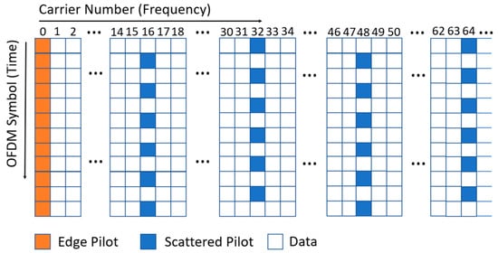
Figure 1.
Scattered-pilot patterns SP 16_2.
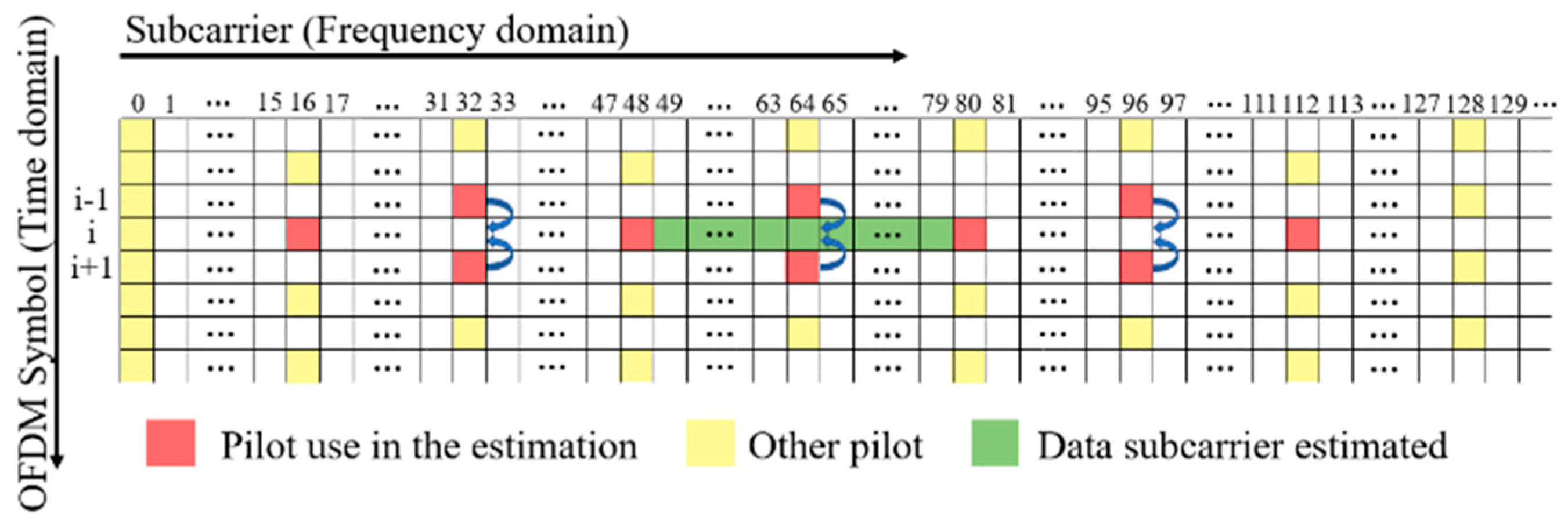
When performing ML-based channel estimation methods, a two-dimensional approach [25] is utilized to find CFRs at the pilot and pseudo-pilot subcarriers, which are then used as inputs for the ML models. The CFR at each pilot subcarrier is first estimated using the LS method. For the channel estimation in the OFDM symbol , pseudo-pilots are used in addition to the pilots in the symbol. The CFRs at pseudo-pilots are obtained by averaging the pilot CFRs at the same subcarriers in symbols and . In Figure 2, the curved arrows indicate how the CFRs at pseudo-pilots are computed. The ML-based channel estimation methods use the CFRs at consecutive pilots in the OFDM symbol and pseudo-pilots in between as features to estimate the CFRs at the data subcarriers between the two neighboring pilots in the center. In Figure 2 with , four pilots and three pseudo-pilots used as features are colored in red, and the data subcarriers estimated are colored in green. Note that is an even integer.
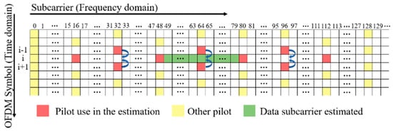
Figure 2.
Pilots, pseudo-pilots, and data subcarriers estimated in ML-based channel estimation methods with .
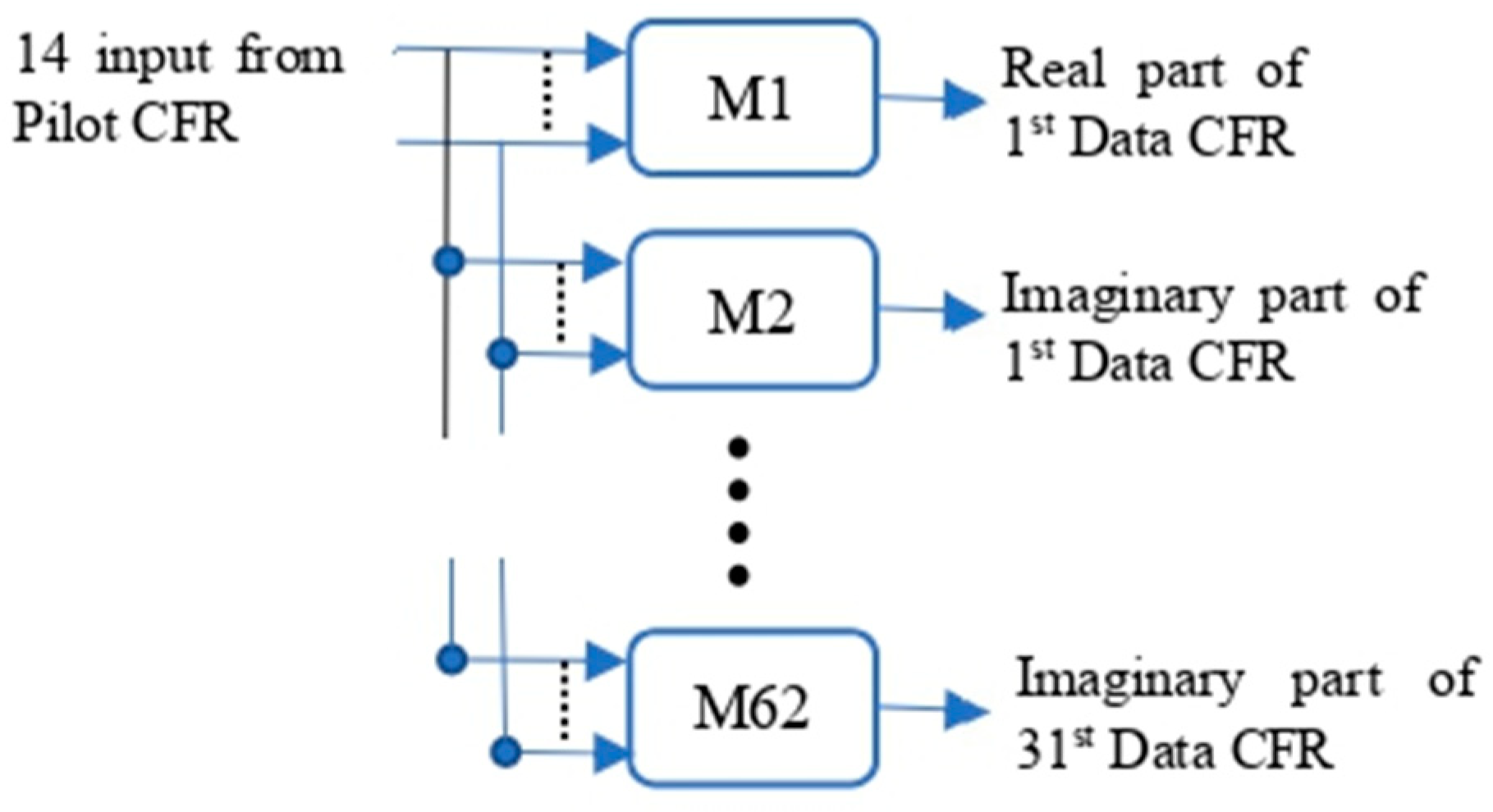
In implementation, as the inputs and outputs of ML models are usually real numbers, the real and imaginary parts of CFRs at the pilots (and pseudo-pilots) are used separately as inputs, and the output is the real part (or imaginary part) of the CFR at one of the data subcarriers estimated. In order to simplify the model design, a model has only one output value. Using Figure 2 with as an example, to estimate the CFRs at all data subcarriers colored in green, one needs models, and each model has input values, as shown in Figure 3. All ML-based estimation methods use the same training data and training process. The training data is obtained from an ATSC 3.0 simulation platform for the experiments in this paper. For a real-world receiver, the receiver first re-encodes and remodulates the decoded data bits to obtain the transmitted symbols and then uses the LS method to obtain the CFRs of data subcarriers for training data. The ML models are described in the next section.

Figure 3.
ML model implementation with .
4. Channel Estimation Methods
This section describes all the ML-based and conventional channel estimation approaches studied in this paper. The ML-based methods, including the linear SVR, SVR with RBF kernel, and DNN, are employed to estimate the channel. The LMMSE and DFT-based interpolation methods are also studied to serve as benchmarks for the performances of the ML-based methods. All ML models’ training data are obtained as described in the previous section. Moreover, the same training data are also available to the LMMSE and DFT-based interpolation methods.
4.1. Linear SVR
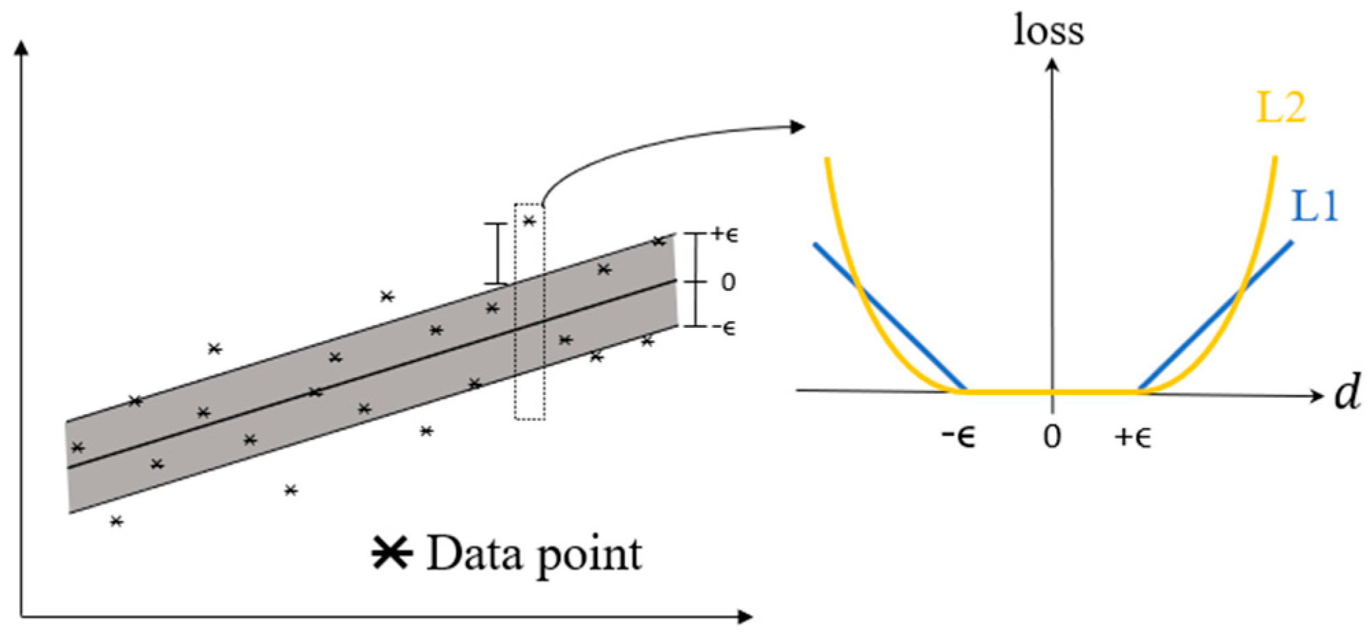
The basic idea of linear SVR is to find a linear function to fit given data points with minimum average loss [16]. Figure 4 depicts the loss for each data point with a distance to the regression line. It shows that only those data points outside the shaded region (i.e., ) are considered when the average loss is calculated. L1 and L2 in the figure represent L1 and L2 loss functions, respectively.
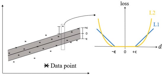
Figure 4.
The losses for data points in linear SVR.
When expressed as an optimization problem, the linear SVR is expressed as follows. Given a set of training pairs , , , the linear SVR solves the following problems [26]
where is the coefficient vector of the linear function, and is a penalty constant. Before conducting the experiments, we must tune the hyperparameters and choose the loss function. Using a grid search with some observations, we conclude that (0.1, 0) is a good choice for the hyperparameters , and the L2 loss function is slightly better than L1. Linear SVR is implemented by the LinearSVR.svm function in sklearn [27]. We will refer to linear SVR as LSVR in the rest of the paper.
4.2. SVR with RBF Kernal
The kernel SVR uses the same concept as the linear SVR. The only difference is that the linear regression line is computed in the kernel-transformed space for kernel SVR. Specifically, the problem is formulated as [28]
where kernel function maps from to feature space, is the target output in the feature space, is a bias term, and and are slack variables introduced to solve the optimization problem. In practice, we usually solve the dual form instead of the primal form in (2). We only have to calculate the inner product of and , denoted as , instead of computing and explicitly. One widely used kernel function is RBF defined by
where is a hyperparameter. This function is observed to be similar to the Gaussian probability density function if we let , where is the variance. The detailed description of the dual form is omitted here. The SVR with RBF kernel is implemented by the svm.SVR function in sklearn [29]. We will refer to this model as SVR-RBF in the rest of the paper. As LSVR, we perform a grid search for the set of hyperparameters for SVR-RBF and find that is a good choice. Note that a minimal means a very large , so the density function is relatively flat around its mean value.
4.3. DNN
In this paper, we study the performance of feedforward multi-layer neural networks in channel estimation. For such a model, the most critical hyperparameters are the number of layers and the number of units in each hidden layer. Again, after some intensive studies, we choose a 6-layer network model (including one input layer, four hidden layers, and one output layer) with network architecture listed in Table 1. The model is implemented using Keras [30], a package on Tensorflow [31]. We will refer to this model as DNN in the rest of the paper.

Table 1.
Hyperparameters of the deep neural network.
4.4. LMMSE-Based Interpolation
When the systems have a comb-type pilot pattern, as in ATSC 3.0, LMMSE channel estimation can be accomplished in two ways. In the first approach, LMMSE is applied to estimate the pilot CFRs, and then an interpolation filter is used to find the CFRs at the data subcarriers. In the second approach, the LMMSE served as both an estimator and an interpolation filter, and thus, the CFRs at data subcarriers are obtained directly. We employ the second approach, which achieves better performance than the first [5]. Let denote the estimated CFRs for pilots and pseudo-pilots. Let denote the CFRs at the data subcarriers. The LMMSE-estimated CFRs at data subcarriers, , are obtained by
where is the covariance matrix of , and is the cross-covariance matrix of and [32]. As the performance of the LMMSE method serves as a benchmark for the performances of the ML-based methods, it is fair to assume that the training data used in the ML-based methods are also available to the LMMSE method. For example, when LMMSE is compared with the ML models with , the LMMSE uses CFR estimates at four consecutive pilots and three pseudo-pilots to estimate CFRs at the 31 data subcarriers in the center, as described in Section 3. Moreover, the two covariance matrixes, and , are obtained by taking the average of and over the training data set, where denotes the Hermitian transpose of a matrix. We will refer to this method as MMSE in the rest of the paper.
4.5. DFT-Based Interpolation
Unlike the MMSE and ML-based estimation methods, the DFT-based interpolation utilizes all pilots and pseudo-pilots in one OFDM symbol to estimate the CFRs at all data subcarriers in the same symbol. First, the estimated CFRs for all pilots and pseudo-pilots are obtained. Second, to reduce the “edge effect” and improve the estimation accuracy [21], virtual pilots are inserted in the guard band (i.e., subcarriers carry zero power) such that there is a pilot, a pseudo-pilot, or a virtual pilot every 16 subcarriers apart in the whole transmission band. The virtual pilots have CFR values equal to the CFR at the nearest pilot or pseudo-pilot. Let denote the pilot CFR vector that contains the CFRs at all pilots, pseudo-pilots, and virtual pilots. In the experiments, the fast Fourier transform (FFT) size for ATSC 3.0 is 32768; is a vector. Third, the channel impulse response (CIR) samples are obtained by applying IDFT to . Next, we truncate to consecutive samples and zero-pad the truncated to the FFT size. Finally, by applying FFT to the zero-padded CIR, we obtain the interpolated CFRs at all data and pilot subcarriers. By controlling , we want to remove excessive noise appearing on the tail parts of the CIR and retain most of the CIR in the meantime. However, it is tricky to determine a good value of (referred to as window length hereafter). On the one hand, a small may remove a portion of critical CIR. On the other hand, a large retains most of the noise. As this method is compared with the ML-based methods, it is fair to assume that the CFRs available for training ML models are also available to the DFT-based interpolation method and are used to find the optimal value of . We will refer to this method as DFT in the rest of the paper.
5. Simulation Results for Linear Channels
The experiments are conducted on an ATSC 3.0 simulation platform with parameters listed in Table 2. The linear channels considered include Typical Urban (TU)-6 [33], UK Long Delay (LD) [34], Brazil B [34], and Brazil D [34], all with zero speed. The delay profiles of these channels are listed in Table 3. TU-6 has the shortest delay spread among the four channel models, whereas LD has the longest.
Table 2.
System parameters used in the experiments.
Table 3.
Delay profiles, delay (μs), and power (dB) for each path of the channel models.
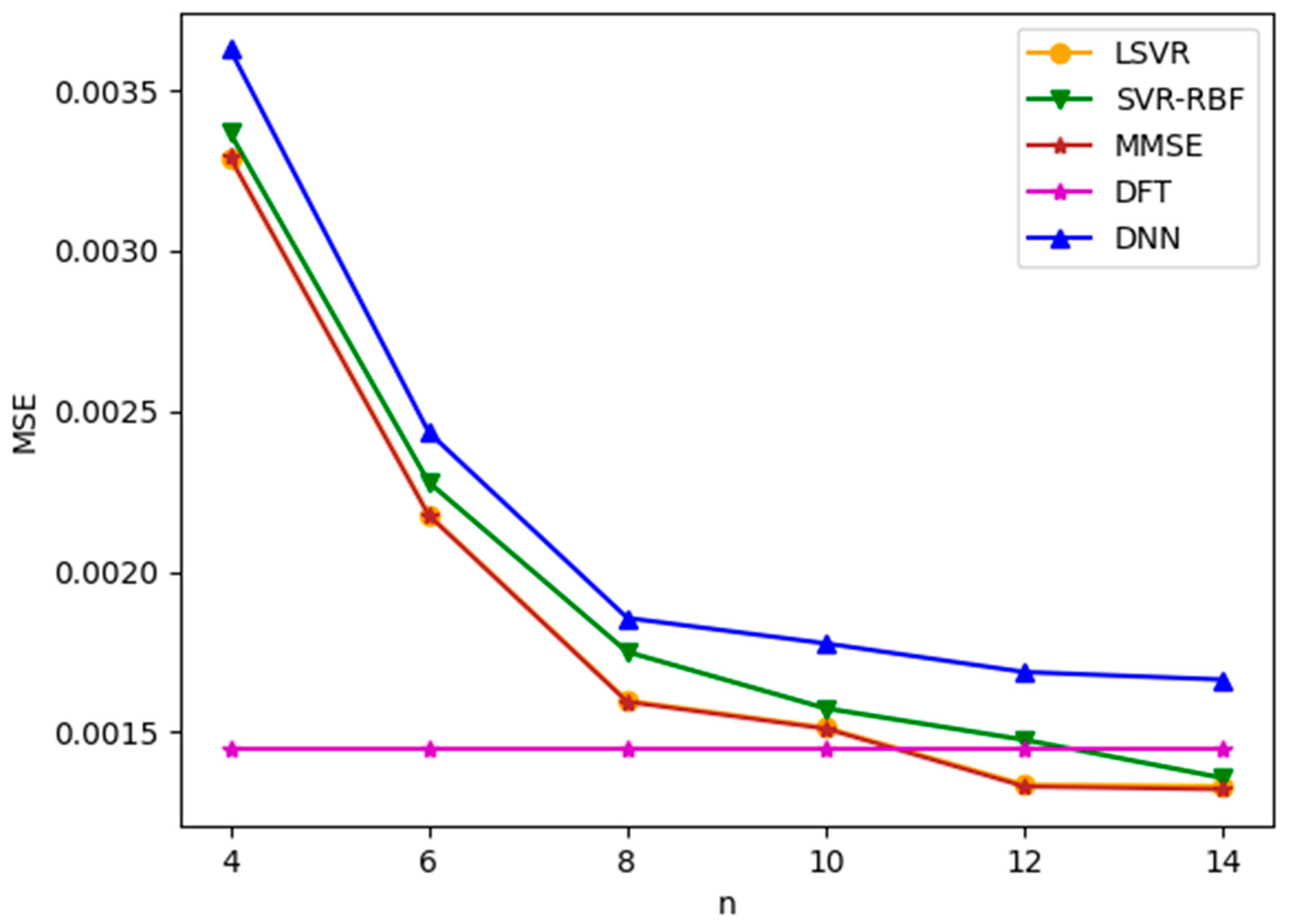
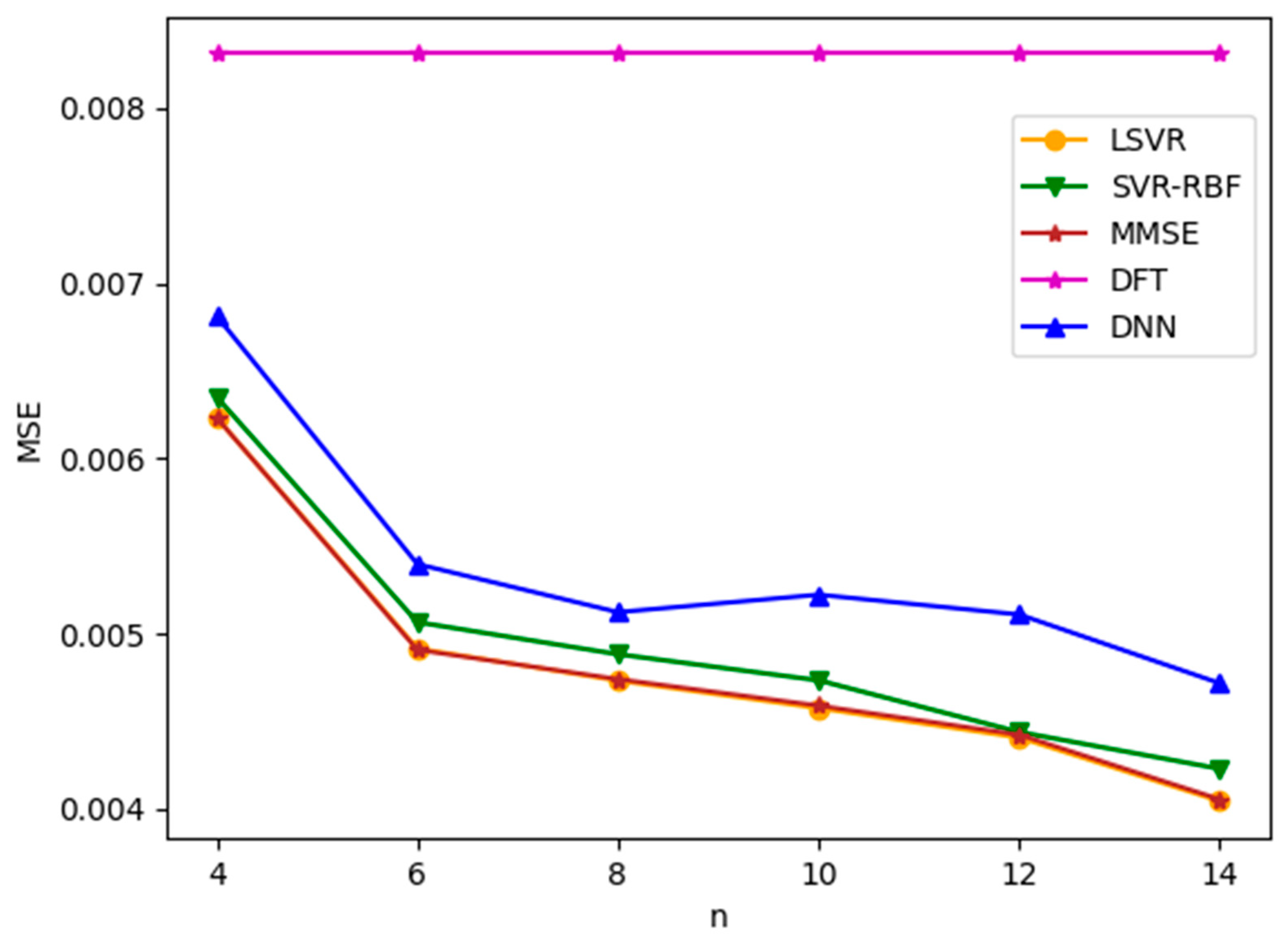
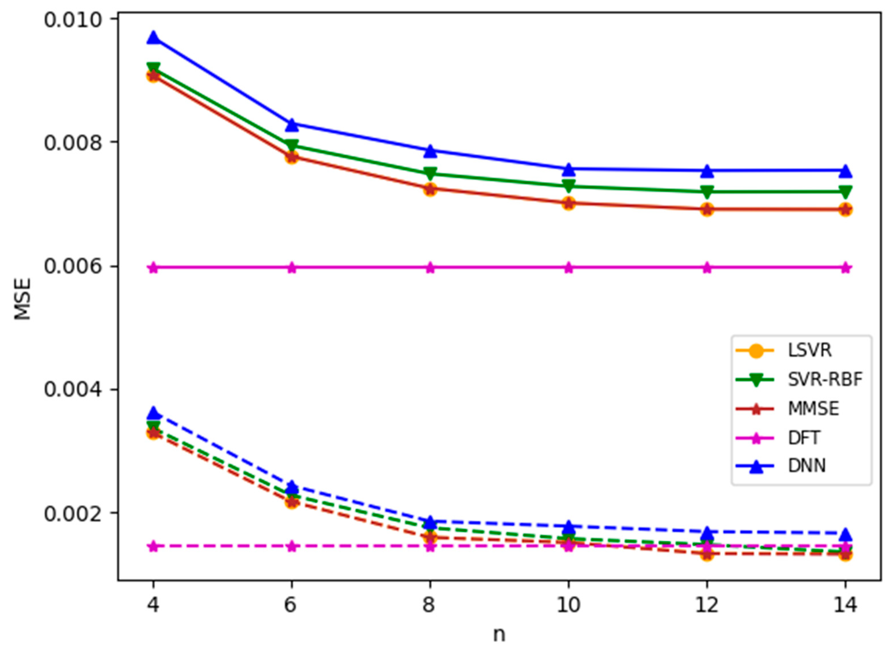
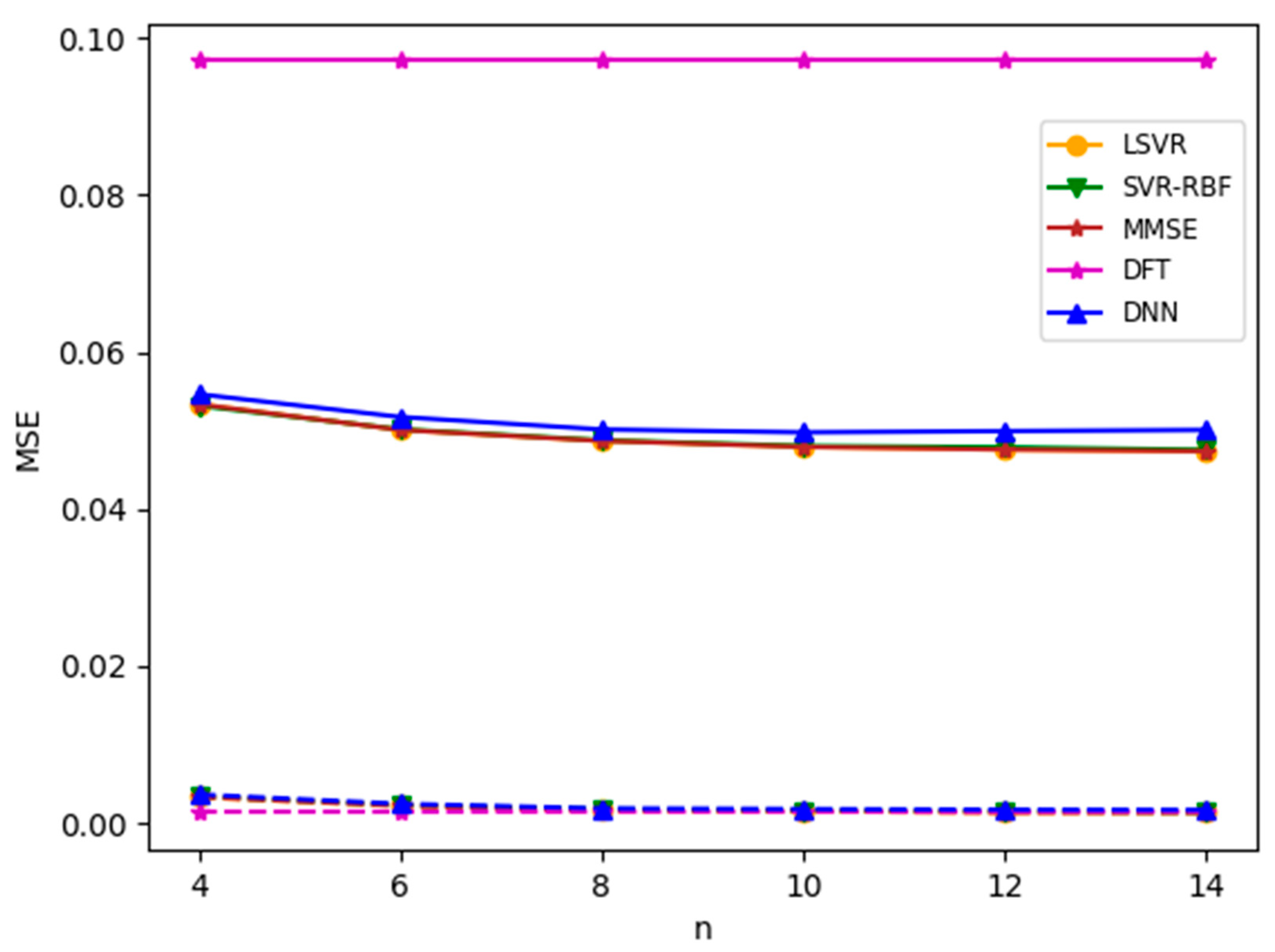
We first apply ML-based channel estimation methods to TU-6 and LD channel models. Figure 5 and Figure 6 plot the channel estimation MSE versus , the number of consecutive pilots used in the ML-based channel estimation methods, for TU-6 and LD channels with an SNR value of 8 dB, respectively. Note that SNR is defined as in this paper. From the figures, it is observed that all three ML-based methods yield similar results. Among them, LSVR achieves the best performance and is almost as good as the best MMSE method. Furthermore, the MSEs of MMSE and the three ML methods decrease as increases. However, for the TU-6 channel in Figure 5, the improvement in MSEs slows down after . This is because the delay spread of TU-6 is short, which leads to slowly changing CFR between neighboring pilot subcarriers. Therefore, increasing the number of pilots after provides little additional channel characteristics to improve the channel estimation significantly. In contrast, the MSE improvement attained by increasing the pilots after is more marked in the LD channel, as shown in Figure 6, because the LD channel has a longer delay spread than the TU-6 channel, which leads to more rapid CFR fluctuation between neighboring pilots. Consequently, the channel estimation module can utilize more pilots to smooth the fluctuation. Figure 5 and Figure 6 show that the LSVR’s MSE performance is almost as good as the best MMSE method for both multipath delay profiles. Moreover, the most cost-effective number of pilots increases as the multipath delay spread increases. The DFT method utilizes all pilots and pseudo-pilots in an OFDM symbol for estimation. Thus, the MSE of DFT does not depend on , as shown in Figure 5 and Figure 6. The performance of DFT is susceptible to the window length. Since the LD channel has a longer delay spread than the TU-6 channel, the optimized window length for the LD channel is much larger than that for the TU-6 channel. In other words, the windowing process leaves more noise for the LD channel, which leads to a larger MSE in Figure 6.
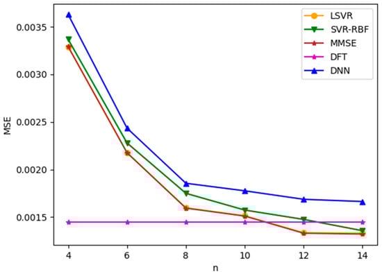
Figure 5.
MSE versus for TU-6 channel with SNR = 8 dB.
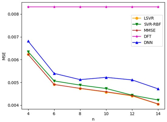
Figure 6.
MSE versus for LD channel with SNR = 8 dB.
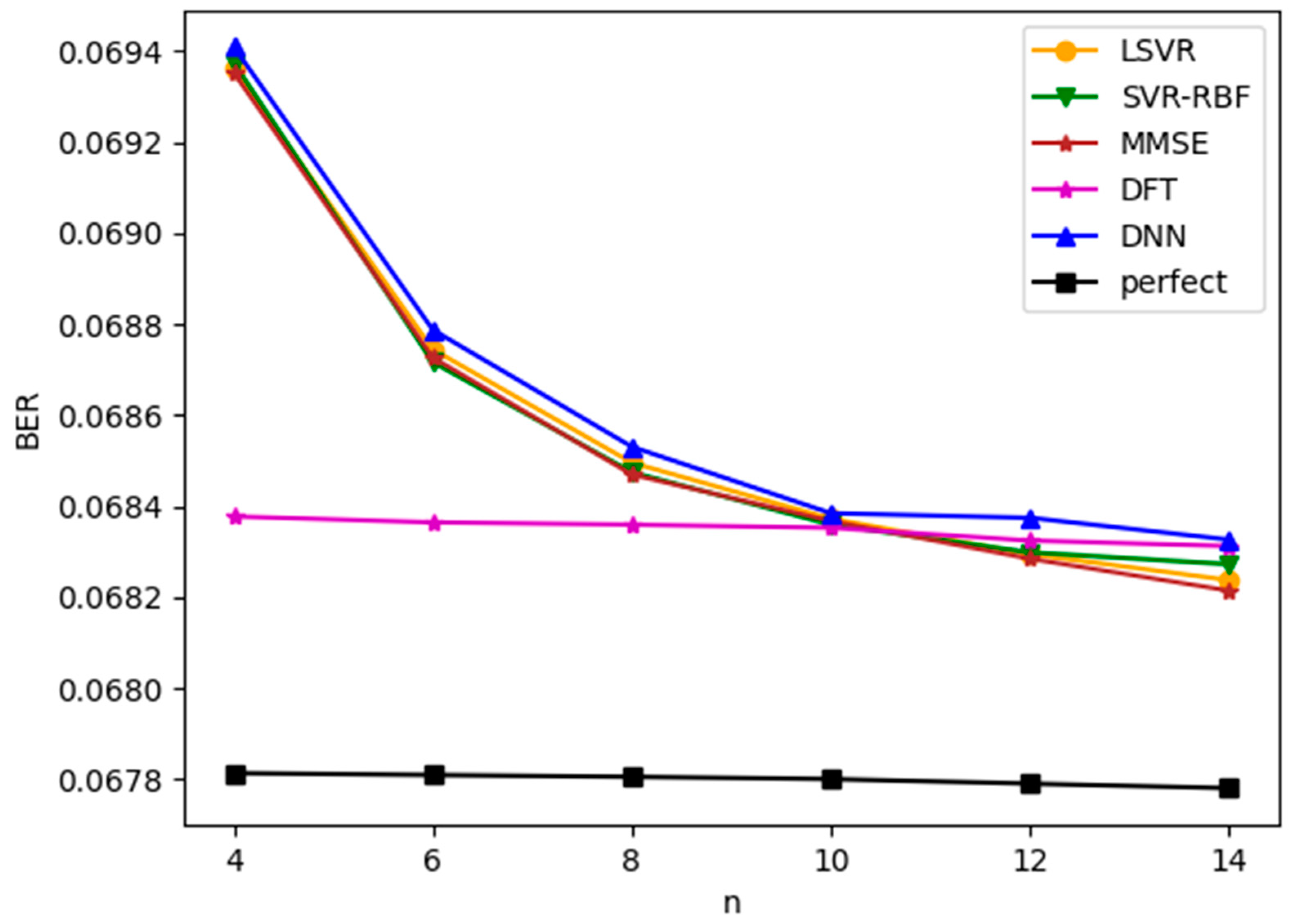
Figure 7 plots the bit error rate (BER) of demodulated bits versus for TU-6 channels with an SNR value of 8 dB. This figure is similar to Figure 5, except BER, instead of channel estimation MSE, is now used as the basis for performance evaluation. The same observations about the performances of the estimation methods can be drawn from Figure 5 and Figure 7. With this observation, we will only provide MSE information in the rest of the paper.
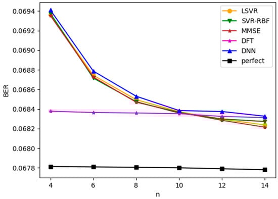
Figure 7.
BER versus for TU-6 channel with SNR = 8 dB.
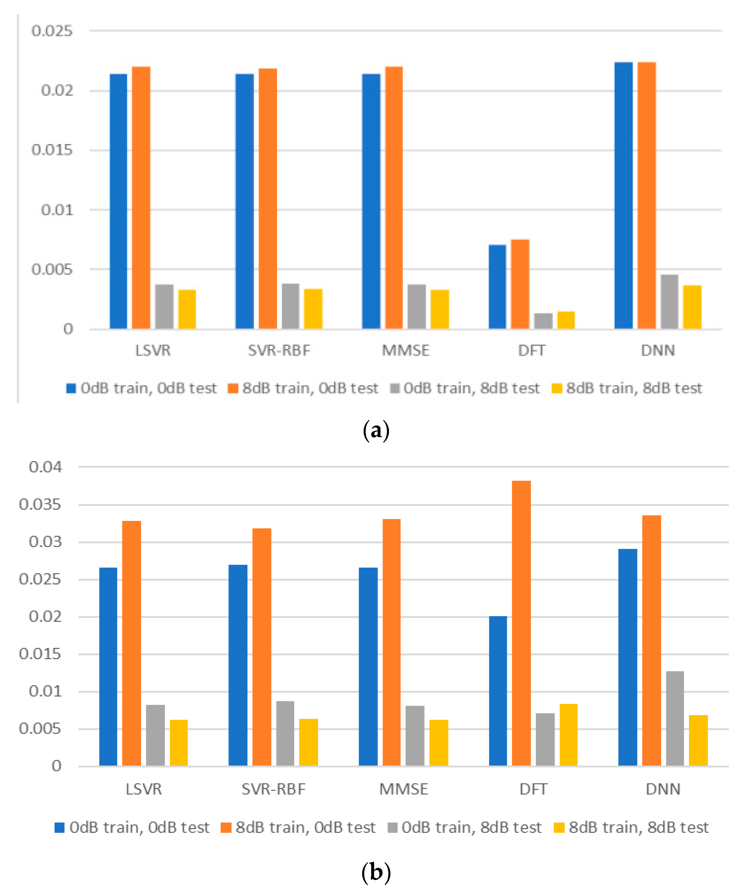
Most papers about channel estimation assume that the training and test channels have the same channel statistics. This assumption, however, is overly simplified and does not reflect real-life situations. In real life, the receiver cannot be sure that the training channel has the same statistics as the test channel. Thus, we would like to evaluate the robustness of the channel estimation methods by considering that the training and test channels have mismatched SNR values or mismatched delay profiles. Figure 8 plots the MSE for TU-6 and LD channels with matched and mismatched SNR values, where for all methods except DFT. The experiment’s training and test channels have 0 or 8 dB SNR values. It is observed that a mismatch of SNR in training and test channels does not seriously degrade the estimation performance for the TU-6 channel. However, the degradation is more noticeable for the LD channel. Therefore, it is advisable for the receiver to accurately estimate the incoming signal’s SNR and use a training model with a closely matched SNR.
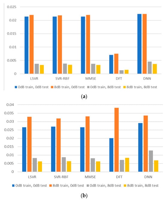
Figure 8.
MSEs for mismatched SNR values: (a) TU-6 channel; (b) LD channel.
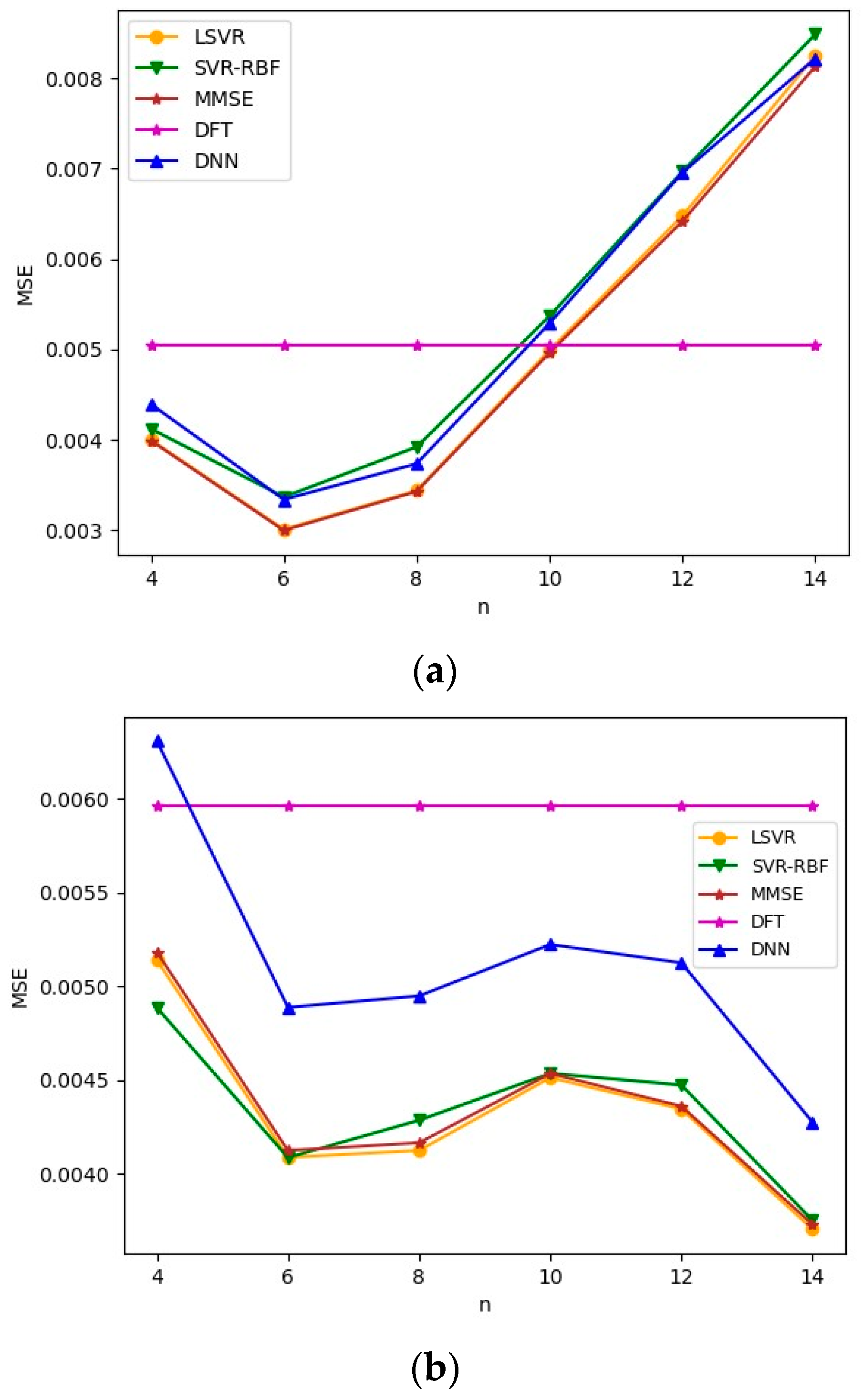
Next, we evaluate the robustness of the channel estimation methods by considering mismatched delay profiles for the training and test channels. In the first experiment, we used TU-6 or LD channels to train the channel estimation modules and used the Brazil B channel as the unknown test channel. The training and test channels have the same SNR set to 8 dB. The MSEs are plotted in Figure 9. If the delay profile of the test channel is close to that of the training channel, such as Brazil B and TU-6 in Figure 9a, the MSE performance is acceptable for small . However, when , the MSE increases rapidly as increases. From the machine learning point of view, a model with a large fits the training channel more perfectly than a model with a smaller . Therefore, the discrepancy between the training and test channels becomes an important factor in MSE performance for large . If the delay profile of the test channel is very different from that of the training channel, such as Brazil B and LD in Figure 9b, the MSE performance degrades even for a small value of , compared with Figure 9a. Although the MSE performance of Figure 9b catches up with that of Figure 9a when is large, it nevertheless indicates that this channel model trained using the LD channel is relatively computationally inefficient.
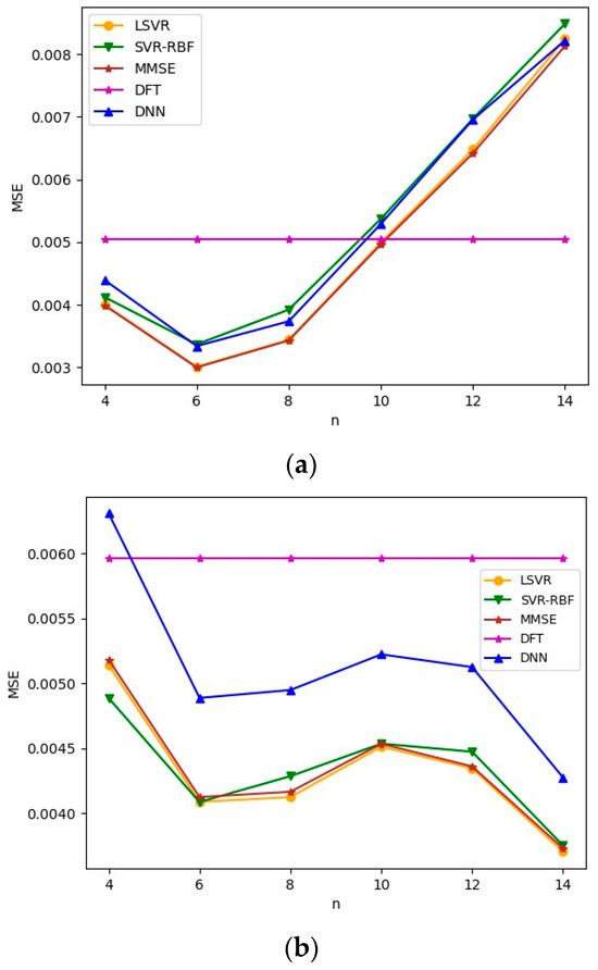
Figure 9.
MSEs for mismatched delay profiles when Brazil B is the test channel model. SNR = 8 dB. (a) TU-6 is the training channel model; (b) LD is the training channel model.
We repeat the above experiment with Brazil D as the test channel. The results are given in Figure 10. We note that all the observations made for Figure 9 remain true for Figure 10. Comparing Figure 9a and Figure 10a, it is observed that as the Brazil D channel has a delay spread comparable to TU-6, the MSE for the Brazil D test channel is lower than that of the Brazil B test channel. When comparing Figure 9b and Figure 10b, it is observed that both have comparable MSEs, although Brazil D has a slight advantage when is large.
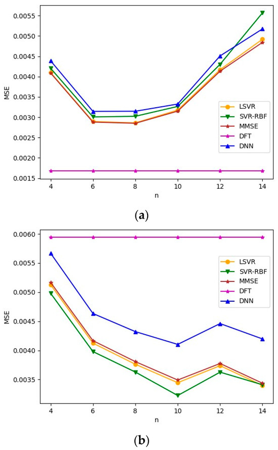
Figure 10.
MSEs of mismatched delay profiles when Brazil D is the test channel model. SNR = 8 dB. (a) TU-6 is the training channel model; (b) LD is the training channel model.
6. Simulation Results for Nonlinear Channels
The nonlinear channel experiments are conducted on the same simulation platform with the same system parameters as the linear channel experiments in the last section. We consider the channel nonlinearity caused by either envelope clipping or nonzero vehicle speed. High peak-to-average power ratio (PAPR) is one of the most common problems in OFDM. The OFDM signal with high PAPR is clipped when passed through a nonlinear high-power amplifier at the transmitter, resulting in a nonlinear channel [35]. A clipping ratio (CR) controls the degree of nonlinearity [20]. Let be the clipping threshold. When the time-domain sample of the complex envelope, , passes through the transmitter amplifier, the clipped output is
The CR is defined as
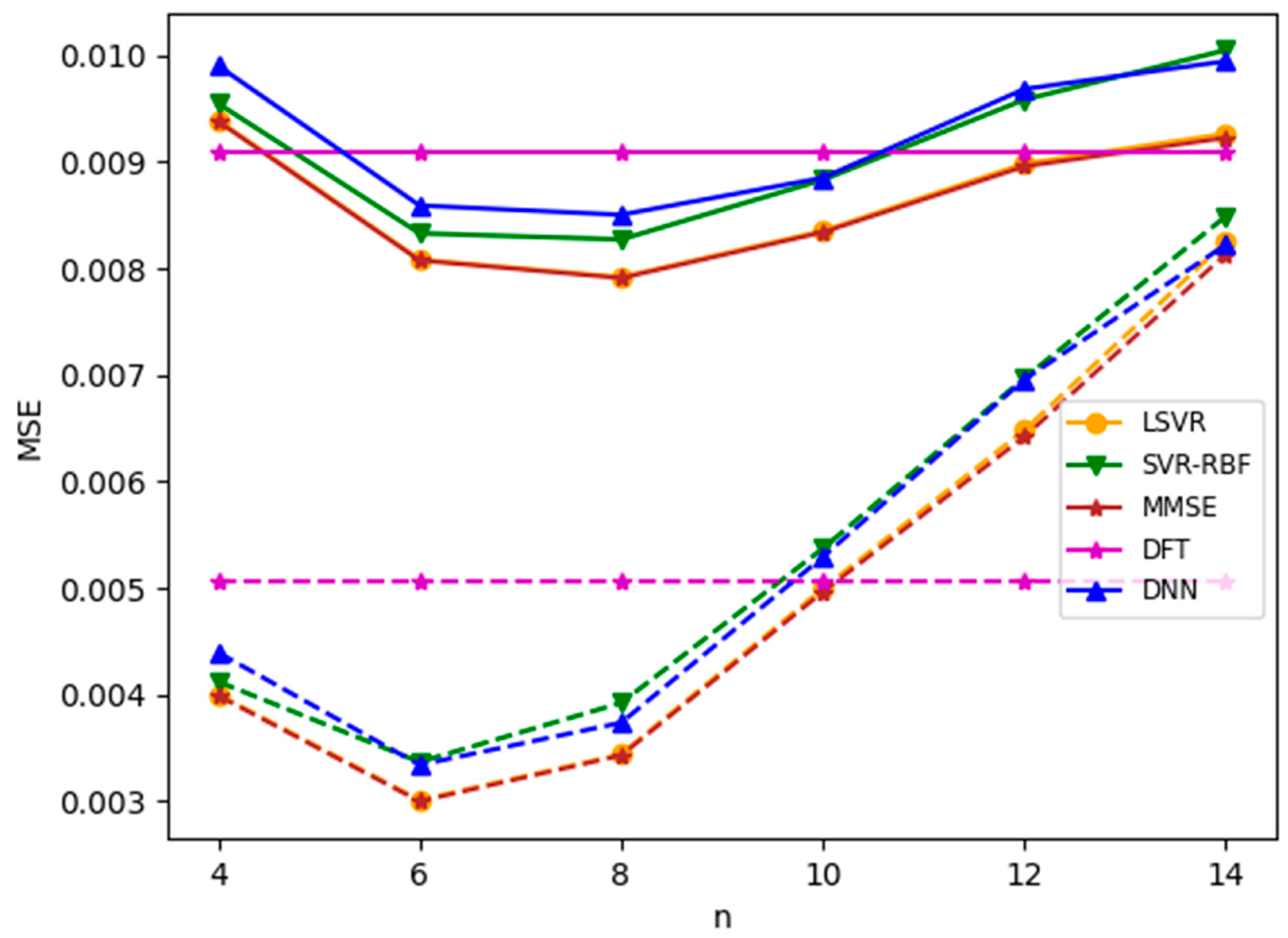
where is the root mean square of the envelope. In the following experiments, if clipping occurs in the channel model, we set CR to 1.7, corresponding to the case that samples are clipped 5.5% of the time. We first apply the channel estimation methods to the TU-6 channel with clipping. Note that in the experiment, both the training and test channel models are TU-6 with clipping. Figure 11 plots the MSE results for an SNR value of 8 dB. It is observed that clipping significantly degrades the MSE performance. Furthermore, contrary to common belief, the DNN model offers no advantage in this nonlinear channel.
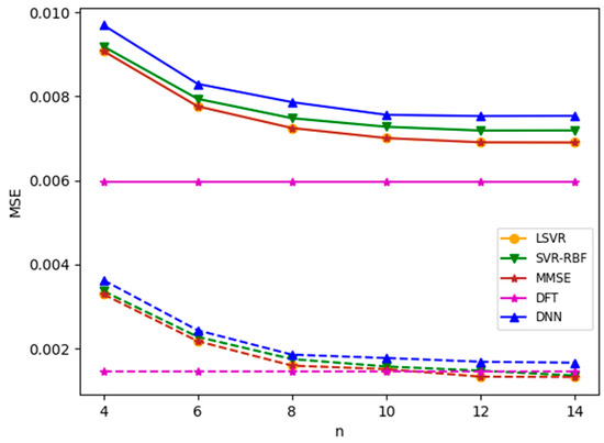
Figure 11.
MSEs for the TU-6 channel with and without clipping. SNR = 8 dB. Solid lines: with clipping (CR = 1.7); dotted line: without clipping.
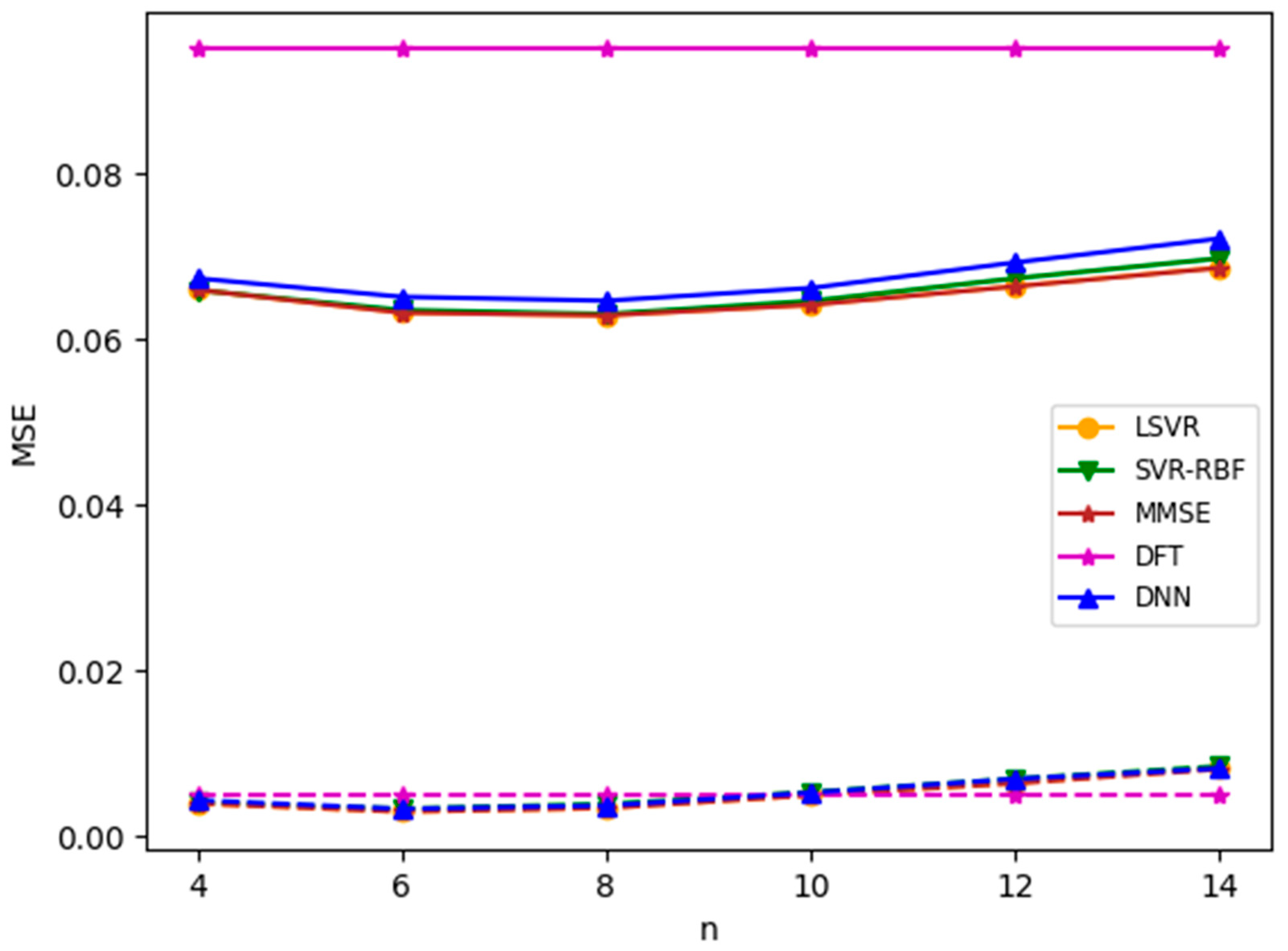
Next, we consider the channel with nonzero vehicle speed. In the following experiments, if the channel model has nonzero vehicle speed, the speed is set to a moderate speed of 69 km/h, corresponding to a maximum Doppler shift of 38.3 Hz. Compared with the subcarrier spacing of 210.94 Hz, the Doppler shift, in the worst case, is more than 18% of the subcarrier spacing. Consequently, the nonzero speed introduces a significant intercarrier interference (ICI) to the channel. The simulation results for the TU-6 channel with nonzero vehicle speed and SNR = 8 dB are plotted in Figure 12. It is observed that the nonzero speed drastically degrades the MSE performance. Furthermore, contrary to common belief, the DNN model offers no advantage in this nonlinear channel. In the figure, all of the methods except DFT have similar MSE performances. In contrast, the performance of DFT suffers more substantial degradation from the nonzero vehicle speed than others. This is because the CFRs at pseudo-pilots are estimated by time-domain interpolation (as described in Section 3), which is quite unreliable with a vehicle speed of 69 km/h. In MMSE and ML-based methods, training data are used to modify the relationship (like weights) between the CFRs at pseudo-pilots and the output estimates. The lack of such a mechanism in DFT is accountable for its large MSE.

Figure 12.
MSEs for TU-6 channel with zero and nonzero speed. SNR = 8 dB. Solid lines: speed 69 km/h; dotted line: speed 0 km/h.
No matter how hard we tune the hyperparameters of the DNN model, such as the number of layers and the number of nodes in each layer, we cannot discover a good DNN model to outperform the other methods considered. First, consider the effect of envelope clipping. The amplitude of a complex envelope sample could be modeled as a (pseudo) random number. Clipping, which could occur in any time-domain sample, introduces additional clipping noise to subcarriers in the frequency domain. As a result, MSE performance for a channel with moderate clipping is similar to that of a linear channel with a smaller SNR value. From this viewpoint, it is unsurprising that DNN has no advantage over the linear methods considered, such as MMSE and LSVR. In the case of the channel with nonzero speed (and thus, nonzero Doppler shift), pilot subcarriers suffer from ICI caused by neighboring data subcarriers. As the DNN model uses only pilot subcarriers as the inputs, it cannot remove or offset the ICI, thus offering no advantage over the linear methods considered. The only possible solution to mitigate ICI is incorporating data subcarriers as inputs into the estimation modules. While theoretically possible, this solution would drastically complicate the design of the channel estimation module in hardware.
Finally, we evaluate the robustness of the channel estimation methods for nonlinear channels by considering mismatched delay profiles. In the following two experiments, we used the TU-6 channel for training and the Brazil B channel for testing. In the first experiment, both training and test channels suffer from clipping; in the second experiment, both training and test channels suffer from nonzero speed. The simulation results for both experiments with an SNR value of 8 dB are plotted in Figure 13 and Figure 14. The results, as expected, show that all the methods considered except DFT have similar performances. DNN does not have any advantage in these experiments. The poor performance of DFT for nonzero speed is due to unreliable CFR estimates at pseudo-pilots, as explained above.
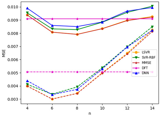
Figure 13.
MSEs of mismatched delay profiles with and without clipping. TU-6 is the training channel; Brazil B is the test channel. Solid lines: with clipping (CR = 1.7); dotted line: without clipping.
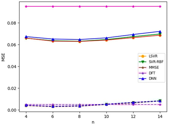
Figure 14.
MSEs of mismatched delay profiles with zero and nonzero speed. TU-6 is the training channel; Brazil B is the test channel. Solid lines: speed 69 km/h; dotted line: speed 0 km/h.
7. Limitations and Discussion
The proposed ML methods’ training is performed offline. Thus, the training process must be repeated in real-world scenarios with dynamic channel variations. Figure 9 and Figure 10 show that the MSE performances of ML-based methods with are sufficiently good, even with mismatched delay profiles for the training and test channels. Therefore, the receiver does not have to repeat the training process frequently. Future work involves designing an online ML-based method to track the dynamic channel variation after the offline ML-based estimation methods proposed in this paper are initially employed.
This paper employs the DNN architecture proposed in [20]. Because the number of output values in our model is less than that in [20], we proportionally scale down the number of nodes in each layer from the one in [20]. As the optimal DNN architecture is an open problem, we cannot be sure whether or not other DNN architectures outperform MMSE. Future work will try other DNN architectures for the channel estimation problem.
Among the proposed ML-based methods, we suggest using the LSVR method for channel estimation. The rationale behind the suggestion is that the LSVR achieves the best performance among all ML-based methods considered while using the least computational resources. Moreover, we suggest using the CFRs of six consecutive pilots and five pseudo-pilots as input features, i.e., . Figure 5 and Figure 6 show that the more pilots used in estimation, the more accurate the estimation results are, but at the cost of increased computational complexity. The improvement of MSE begins to slow down after . In addition, we observe from Figure 9 that with delay profile mismatch, overfitting is setting in after . Combining these two observations, we suggest that is a good choice for the input features.
8. Conclusions
We propose several ML-based channel estimation methods for ATSC 3.0 and find the number of pilots achieving good cost-effectiveness. The simulation results show that all ML-based methods perform almost the same as the LMMSE estimator in linear and nonlinear channel models. Furthermore, contrary to common beliefs, a DNN-based estimation method does not outperform the linear channel estimation methods in nonlinear channels, which suffer from clipping or the Doppler effect. Considering all experimental results, we suggest using the LSVR method with the CFRs at six consecutive pilots and five pseudo-pilots as features for channel estimation in ATSC 3.0 systems.
Author Contributions
Conceptualization, Y.-S.L. and S.D.Y.; methodology, Y.-S.L.; software, Y.-C.L.; formal analysis, Y.-S.L.; writing—original draft preparation, Y.-S.L. and S.D.Y.; writing—review and editing, Y.-S.L. and S.D.Y. All authors have read and agreed to the published version of the manuscript.
Funding
This research was funded by the National Science and Technology Council, Taiwan, grant number NSTC 112-2221-E-027-091 and MOST 111-2637-E-027-005.
Institutional Review Board Statement
Not applicable.
Informed Consent Statement
Not applicable.
Data Availability Statement
The ATSC 3.0 simulation platform used to generate training and test data, the training and test set, and all the ML-based and conventional channel estimation methods evaluated in this paper are uploaded to Google Drive. Readers can find the link at https://github.com/MarquisGramont/ml-channel-estimation-for-atsc3.0 (accessed on 7 June 2024).
Conflicts of Interest
The authors declare no conflicts of interest.
References
- Advanced Television Systems Committee. ATSC Standard: Physical Layer Protocol (A/322), Doc. A/322:2017, Feb. 2017. Available online: https://www.atsc.org/wp-content/uploads/2016/10/A322-2017a-Physical-Layer-Protocol-1.pdf (accessed on 4 June 2024).
- Coleri, S.; Ergen, M.; Puri, A.; Bahai, A. A study of channel estimation in OFDM systems. In Proceedings of the VTC Fall 2002, Vancouver, BC, Canada, 24–28 September 2002. [Google Scholar]
- Ozdemir, M.K.; Arslan, H. Channel estimation for wireless OFDM systems. IEEE Commun. Surv. Tutor. 2007, 9, 18–48. [Google Scholar] [CrossRef]
- Liu, Y.; Tan, Z.; Hu, H.; Cimini, L.J.; Li, G.Y. Channel estimation for OFDM. IEEE Commun. Surv. Tutor. 2014, 16, 1891–1908. [Google Scholar] [CrossRef]
- Savaux, V.; Louët, Y. LMMSE channel estimation in OFDM context: A review. IET Signal Process 2017, 11, 123–134. [Google Scholar] [CrossRef]
- You, S.D.; Chen, K.-Y.; Liu, Y.-S. Cubic convolution interpolation function with variable coefficients and its application to channel estimation for IEEE 802.16 initial downlink. IET Commun. 2012, 6, 1979–1987. [Google Scholar] [CrossRef]
- Adegbite, S.A.; Stewart, B.G.; McMeekin, S.G. Least squares interpolation methods for LTE system channel estimation over extended ITU channels. Int. J. Inf. Electron. Eng. 2013, 3, 414–418. [Google Scholar]
- Seo, J.; Kim, D.K. DFT-based interpolation with simple leakage suppression. IEICE Electron. Express 2011, 8, 525–529. [Google Scholar] [CrossRef]
- Kang, Y.; Kim, K.; Park, H. Efficient DFT-based channel estimation for OFDM systems on multipath channels. IET Commun. 2007, 1, 197–202. [Google Scholar] [CrossRef]
- Bossert, M.; Donder, A.; Zyablo, V. Improved channel estimation with decision feedback for OFDM systems. Electron. Lett. 1998, 34, 1064–1065. [Google Scholar] [CrossRef]
- Liu, Y.-S.; You, S.D.; Wu, R.-K. Burst allocation method to enable decision-directed channel estimation for mobile WiMAX downlink transmission. EURASIP J. Wirel. Commun. Netw. 2013, 2013, 153. [Google Scholar] [CrossRef]
- Qin, Z.; Ye, H.; Li, G.Y.; Juang, B.-H.F. Deep learning in physical layer communications. IEEE Wirel. Commun. 2019, 26, 93–99. [Google Scholar] [CrossRef]
- Huang, H.; Guo, S.; Gui, G.; Yang, Z.; Zhang, J.; Sari, H.; Adachi, F. Deep learning for physical-layer 5G wireless techniques: Opportunities, challenges and solutions. IEEE Wirel. Commun. 2020, 27, 214–222. [Google Scholar] [CrossRef]
- Wang, Z.; Wei, S.; Zou, L.; Liao, F.; Lang, W.; Li, Y. Deep-Learning-Based Carrier Frequency Offset Estimation and Its Cross-Evaluation in Multiple-Channel Models. Information 2023, 14, 98. [Google Scholar] [CrossRef]
- Razzaq, H.S.; Hussain, Z.M. Instantaneous Frequency Estimation of FM Signals under Gaussian and Symmetric α-Stable Noise: Deep Learning versus Time–Frequency Analysis. Information 2023, 14, 18. [Google Scholar] [CrossRef]
- Smola, A.J.; Schölkopf, B. A tutorial on support vector regression. Stat. Comput. 2004, 14, 199–222. [Google Scholar] [CrossRef]
- Glorot, X.; Bordes, A.; Bengio, Y. Deep sparse rectifier neural networks. In Proceedings of the AISTATS 2011, Ft. Lauderdale, FL, USA, 11–13 April 2011. [Google Scholar]
- Mei, K.; Liu, J.; Zhang, X.; Rajatheva, N.; Wei, J. Performance analysis on machine learning-based channel estimation. IEEE Trans. Commun. 2021, 69, 5183–5193. [Google Scholar] [CrossRef]
- Hu, Q.; Gao, F.; Zhang, H.; Jin, S.; Li, G.Y. Deep learning for channel estimation: Interpretation, performance, and comparison. IEEE Trans. Wirel. Commun. 2021, 20, 2398–2412. [Google Scholar] [CrossRef]
- Ye, H.; Li, G.Y.; Juang, B. Power of deep learning for channel estimation and signal detection in OFDM systems. IEEE Wirel. Commun. Lett. 2018, 7, 114–117. [Google Scholar] [CrossRef]
- Zhang, L.; Wu, Y.; Li, W.; Kim, H.M.; Park, S.-I.; Angueira, P.; Montalban, J.; Velez, M. Application of DFT-based channel estimation for accurate signal cancellation in cloud-Txn multi-layer broadcasting system. In Proceedings of the BMSB 2014, Beijing, China, 25–27 June 2014. [Google Scholar]
- You, S.D. Channel estimation with iterative DFT-based smoothing for OFDM systems with non-uniformly spaced pilots in channels with long delay spread. IET Commun. 2014, 8, 2984–2992. [Google Scholar] [CrossRef]
- Du, Z.; Song, X.; Cheng, J.; Beaulieu, N.C. Maximum likelihood based channel estimation for macrocellular OFDM uplinks in dispersive time-varying channels. IEEE Trans. Wirel. Commun. 2011, 10, 176–187. [Google Scholar] [CrossRef]
- Yao, R.; Qin, Q.; Wang, S.; Qi, N.; Fan, Y.; Zuo, X. Deep Learning Assisted Channel Estimation Refinement in Uplink OFDM Systems Under Time-Varying Channels. In Proceedings of the 2021 IWCMC, Harbin City, China, 28 June–2 July 2 2021. [Google Scholar]
- Liu, Y.-S.; Huang, C.-H.; You, S.D. Estimation of channel MSE for ATSC 3.0 receiver and its applications. ICT Express 2022, 8, 202–206. [Google Scholar] [CrossRef]
- Fan, R.-E.; Chang, K.-W.; Hsieh, C.-J.; Wang, X.-R.; Lin, C.-J. LIBLINEAR: A library for large linear classification. J. Mach. Learn. Res. 2008, 9, 1871–1874. [Google Scholar]
- Linear SVR, Scikit-Learn 1.4.2. Available online: https://scikit-learn.org/stable/modules/generated/sklearn.svm.LinearSVR.html#sklearn.svm.LinearSVR (accessed on 10 February 2024).
- Vapnik, V.N. Statistical Learning Theory; Wiley: Hoboken, NJ, USA, 1998. [Google Scholar]
- SVR, Scikit-Learn 1.4.2. Available online: https://scikit-learn.org/stable/modules/generated/sklearn.svm.SVR.html#sklearn.svm.SVR (accessed on 10 February 2024).
- Keras. Available online: https://keras.io/ (accessed on 10 February 2024).
- TensorFlow. Available online: https://www.tensorflow.org/ (accessed on 10 February 2024).
- Scharf, L.L. Statistical Signal Processing: Detection, Estimation, and Time Series Analysis; Addison-Wesley: Boston, MA, USA, 1991. [Google Scholar]
- 3GPP, Digital Cellular Telecommunications System (Phase 2+); Radio Transmission and Reception, 3GPP TS 05.05 V.8.20.0 Release1999. Available online: https://www.etsi.org/deliver/etsi_ts/100900_100999/100910/08.20.00_60/ts_100910v082000p.pdf (accessed on 4 June 2024).
- ITU, Guidelines and techniques for the evaluation of digital terrestrial television broadcasting systems, Report ITU-R BT.2035. 2003. Available online: https://www.itu.int/dms_pub/itu-r/opb/rep/R-REP-BT.2035-2003-PDF-E.pdf (accessed on 4 June 2024).
- Li, X.; Cimini, L.J. Effects of clipping and filtering on the performance of OFDM. IEEE Commun. Lett. 1998, 2, 131–133. [Google Scholar]


Disclaimer/Publisher’s Note: The statements, opinions and data contained in all publications are solely those of the individual author(s) and contributor(s) and not of MDPI and/or the editor(s). MDPI and/or the editor(s) disclaim responsibility for any injury to people or property resulting from any ideas, methods, instructions or products referred to in the content. |
© 2024 by the authors. Licensee MDPI, Basel, Switzerland. This article is an open access article distributed under the terms and conditions of the Creative Commons Attribution (CC BY) license (https://creativecommons.org/licenses/by/4.0/).