

The Development of a Prototype Solution for Collecting Information on Cycling and Hiking Trail Users
 and
and 
Abstract
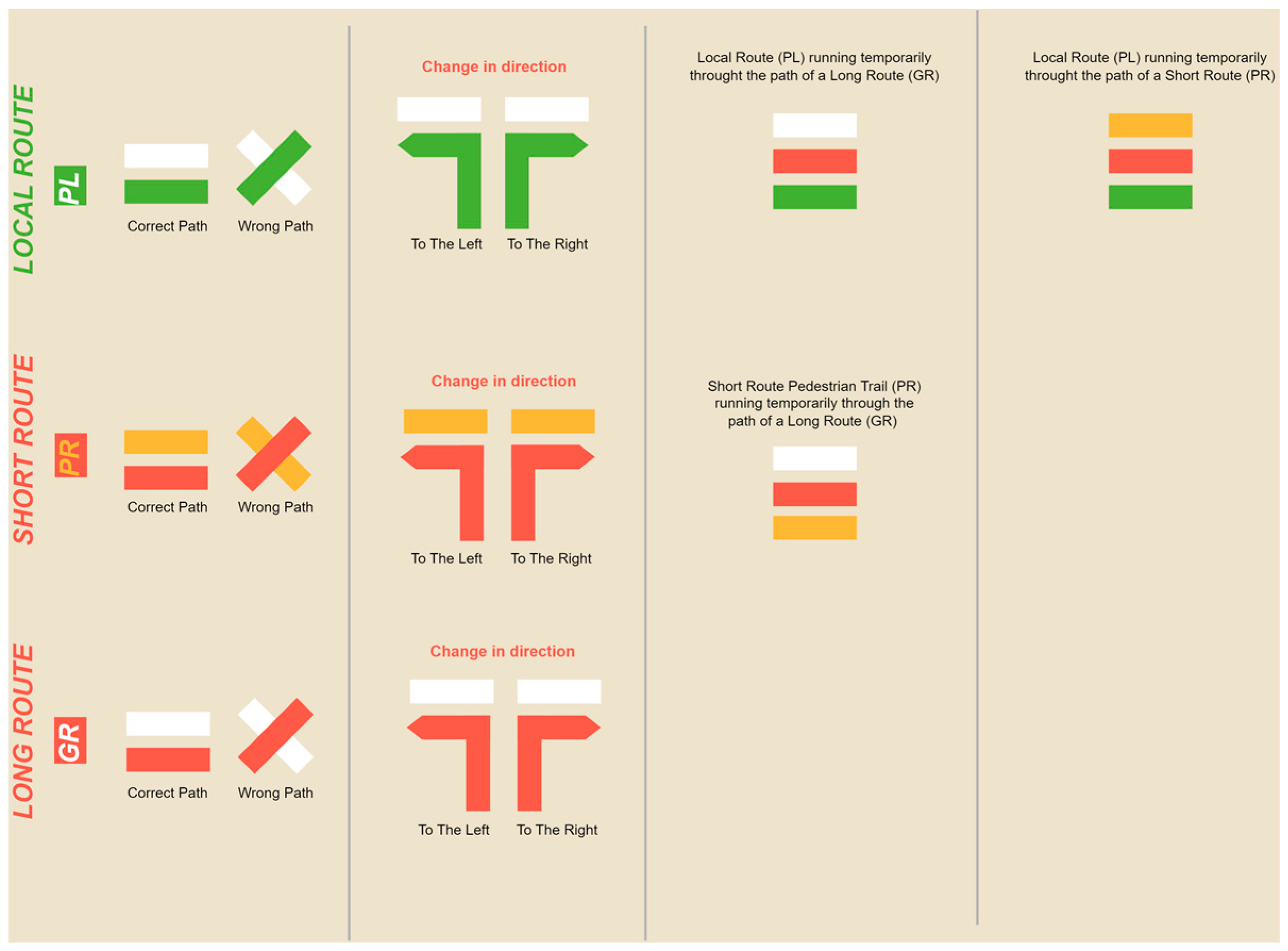
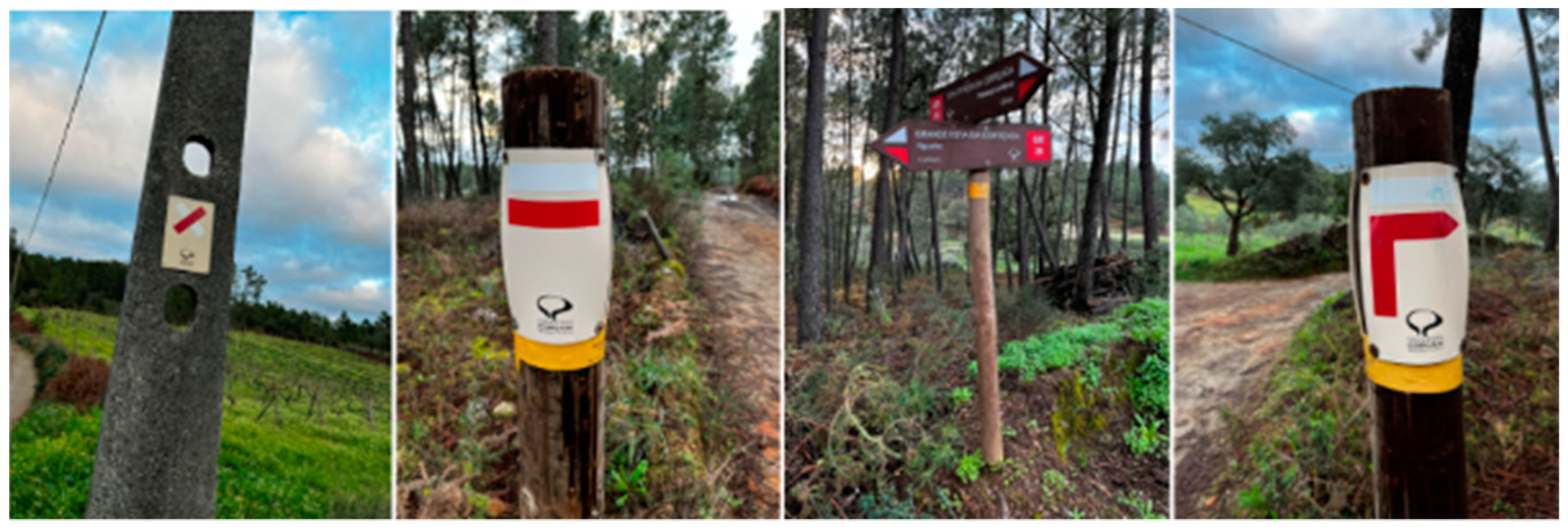
:1. Introduction
2. Prototype
2.1. Architecture
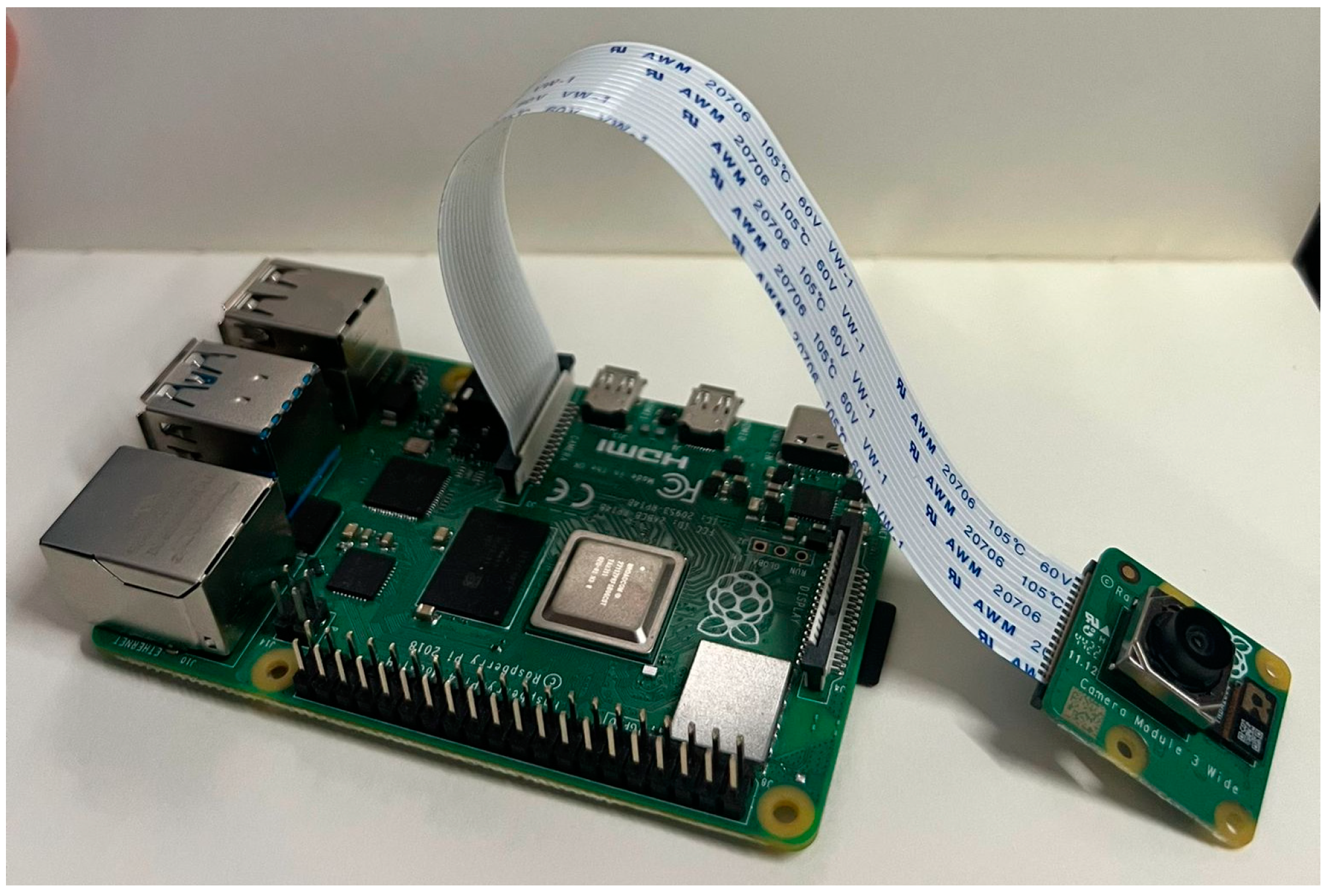
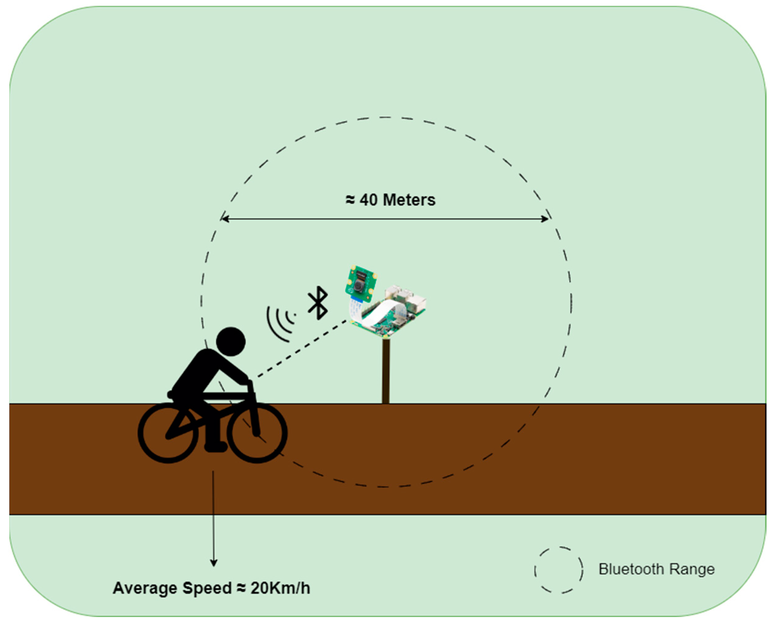
2.2. Hardware Component
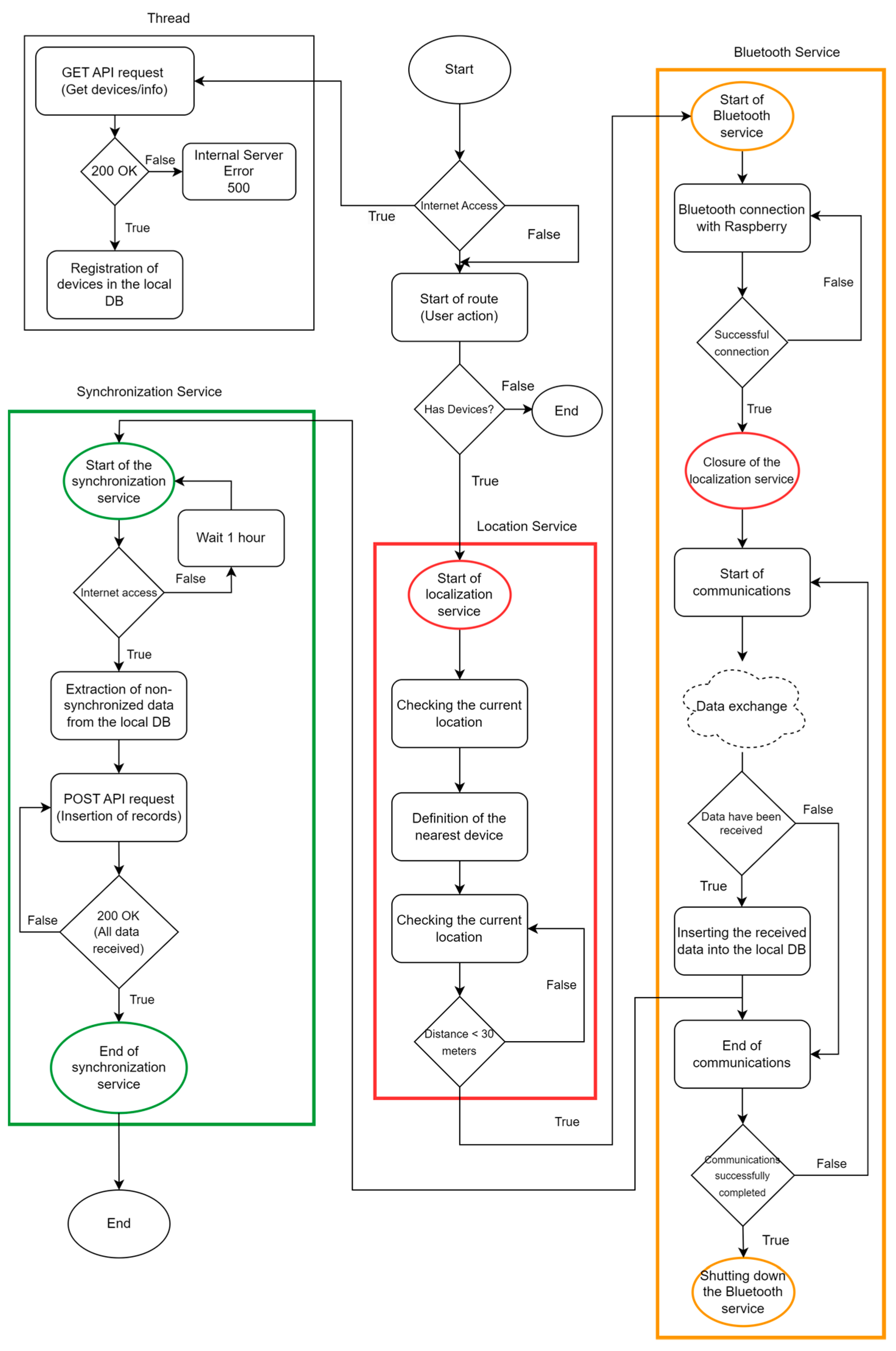
2.3. Software Component
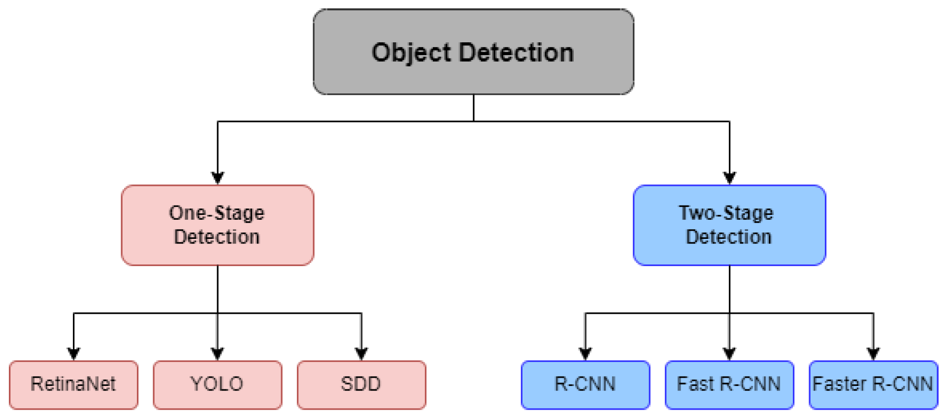
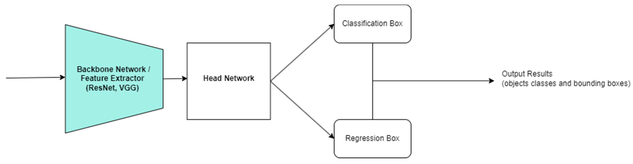
2.3.1. Convolutional Neural Networks
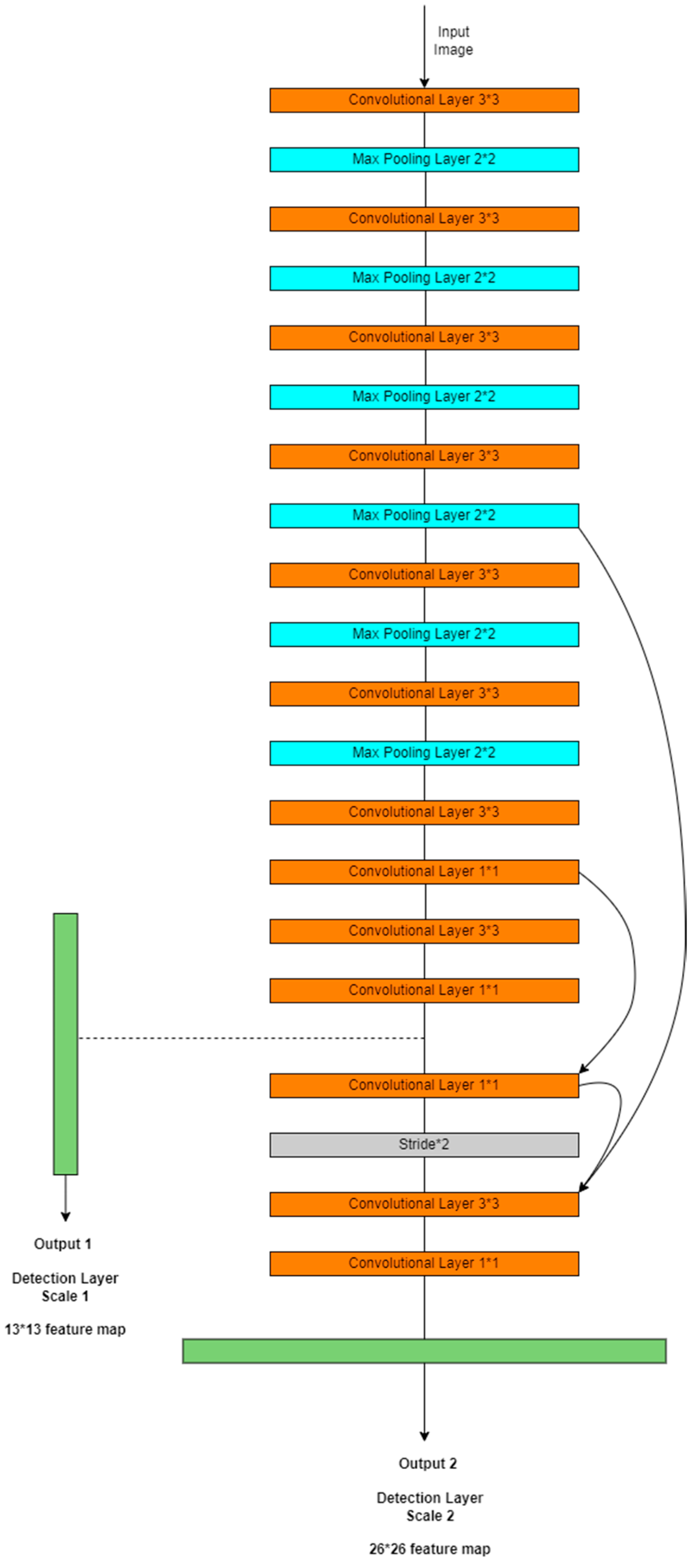
One-Stage Detection
Two-Stage Detection
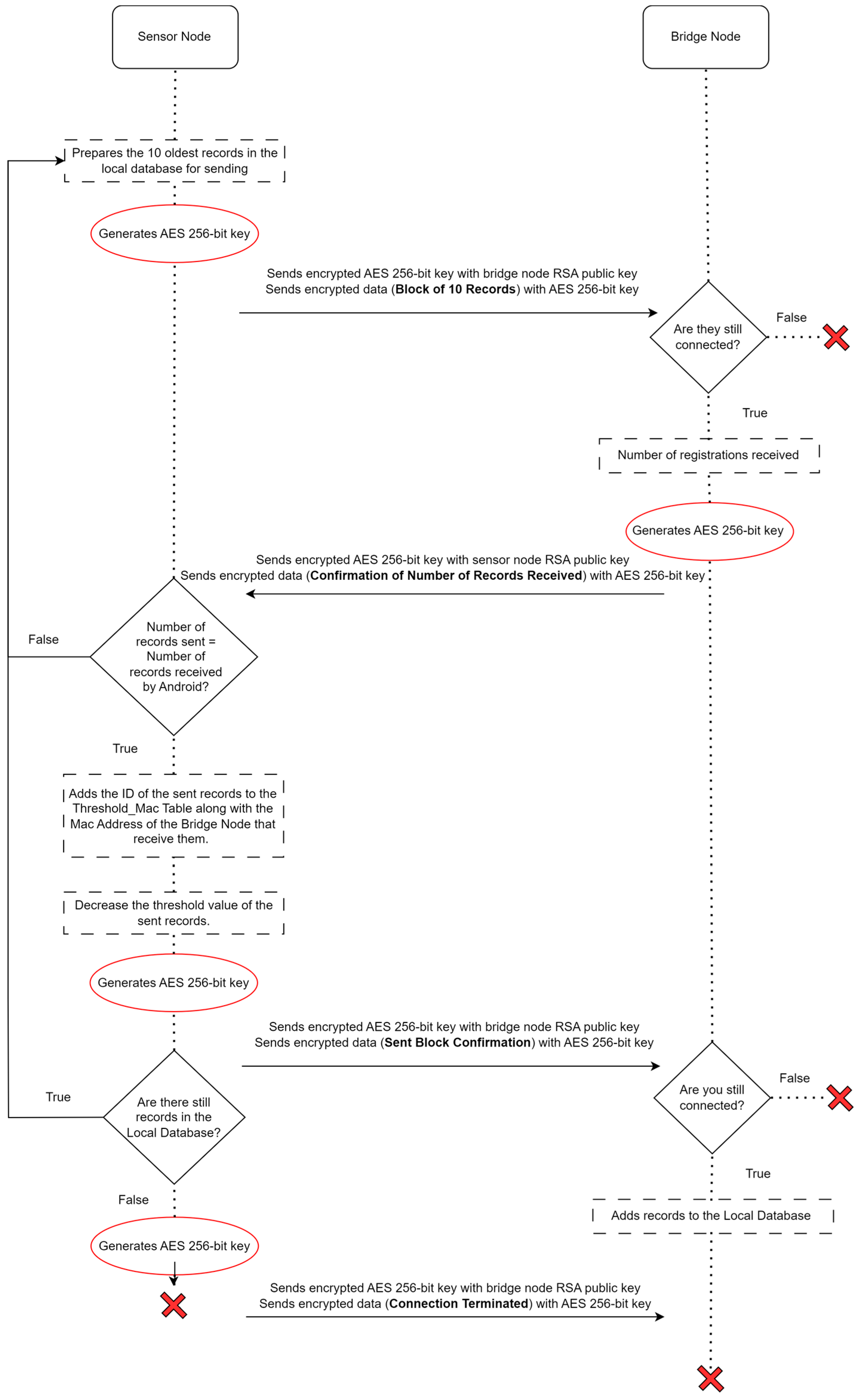
2.3.2. Sensor Node
- Two bytes for “square brackets” for the record array;
- Twenty bytes for “curly braces”, delimiting each record;
- Nineteen bytes for the “commas” separating the name/value array and separating the records;
- Thirty-nine bytes of “spaces” between name/value, between name/value sets and between records (after the comma separating the records);
- Fifty bytes for the name of the class attribute of the 10 records;
- One-hundred bytes for the value of the class attribute of the 10 records;
- Ninety bytes for the name of the timestamp attribute of the 10 records;
- One-hundred and ninety bytes for the value of the timestamp attribute of the 10 records;
- Eighty bytes for the “quotation marks” that are placed in the names and values of the 10 records;
- Twenty bytes for the “colon” to separate the names from the values of the 10 records;
- Thirty-two bytes for the AES-256-bit symmetric key.
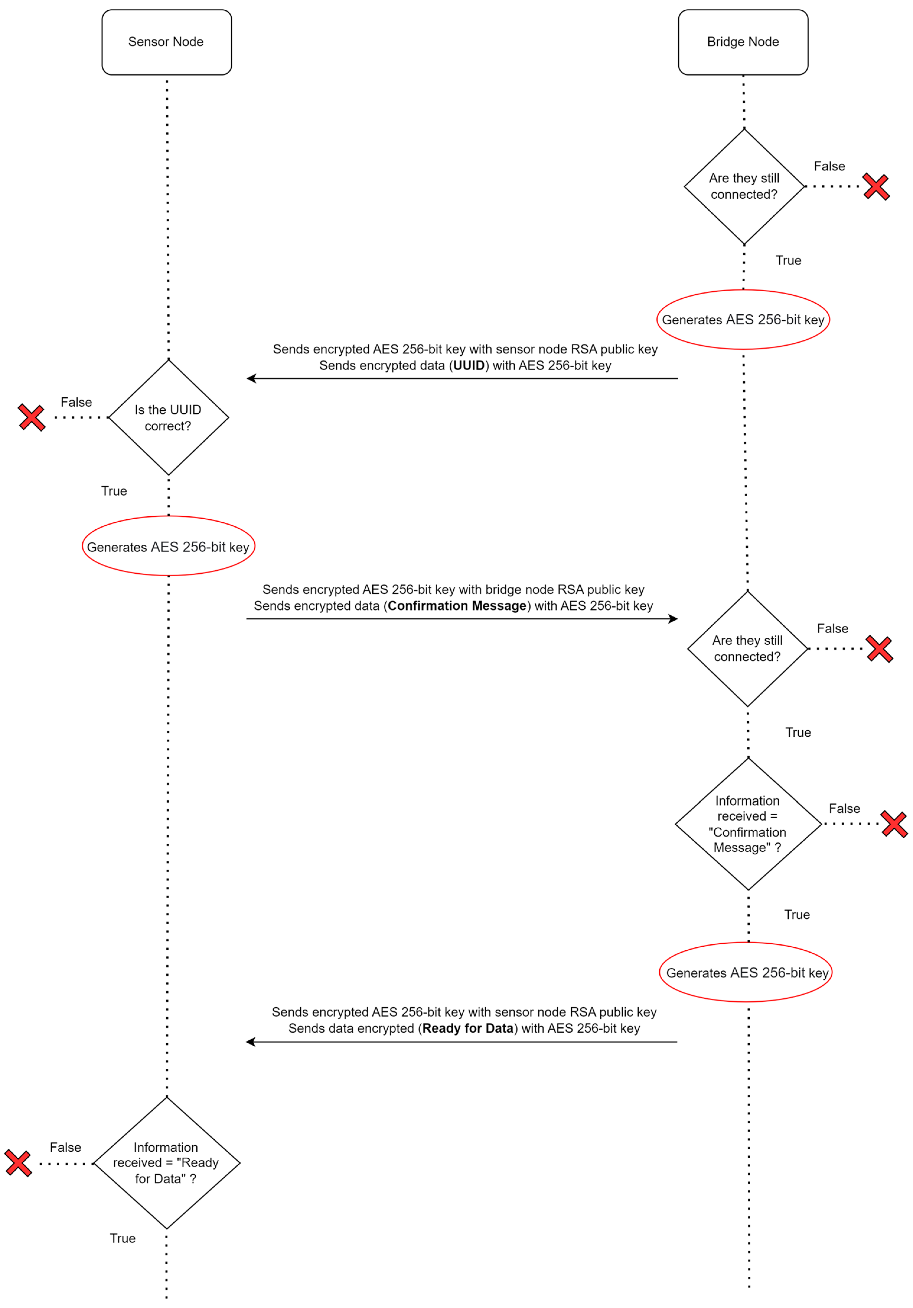
2.3.3. Bridge Node
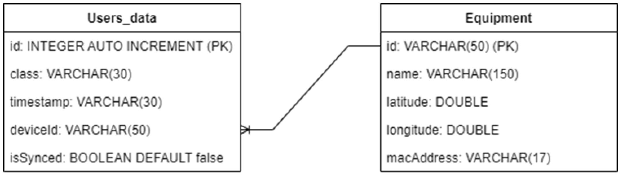
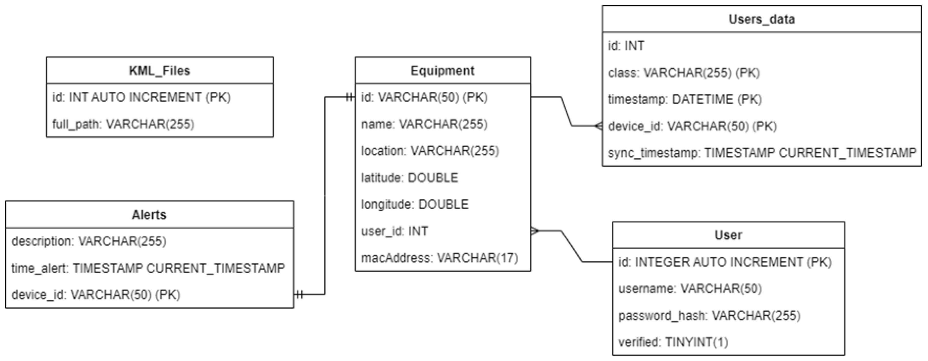
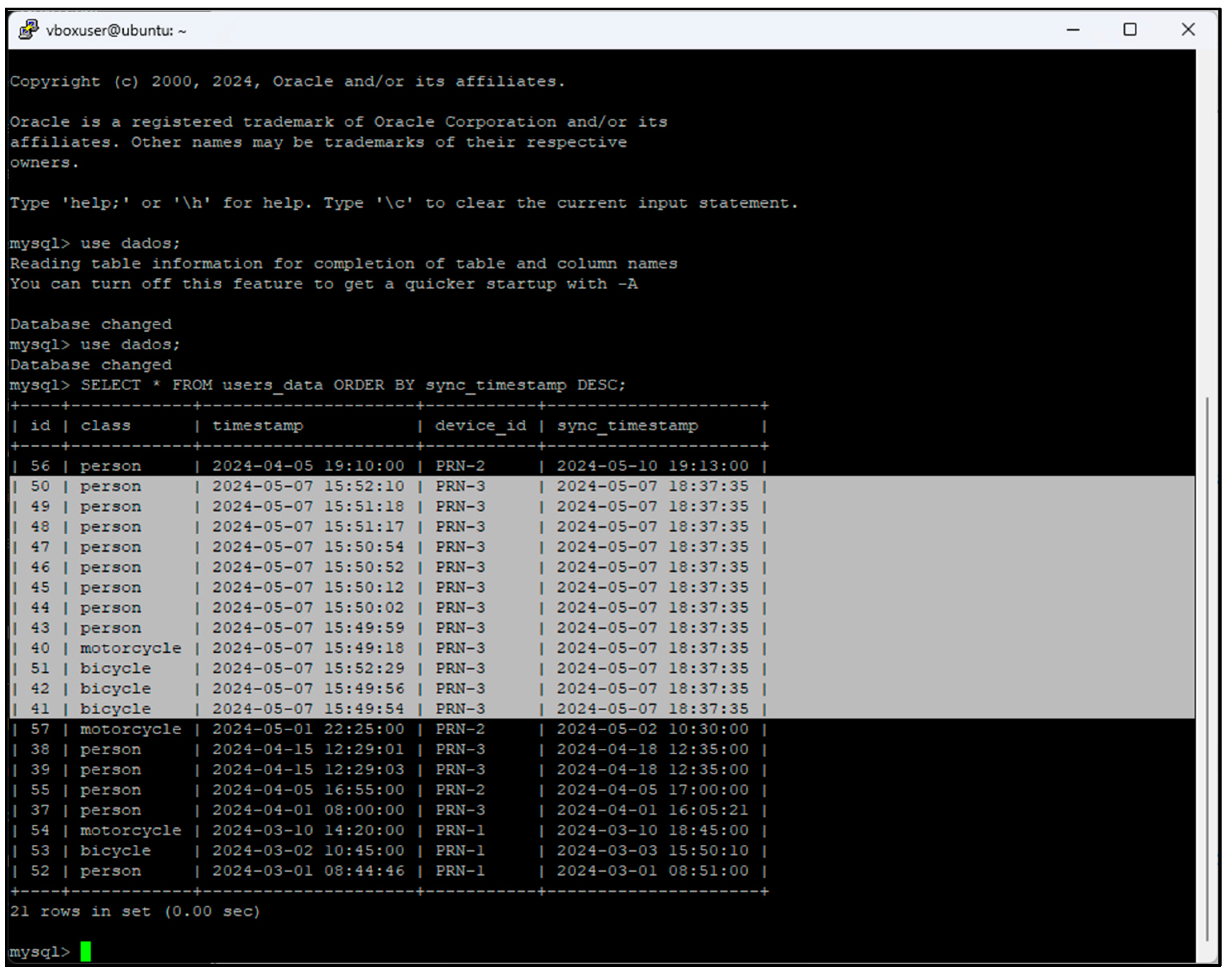
2.3.4. Central Database
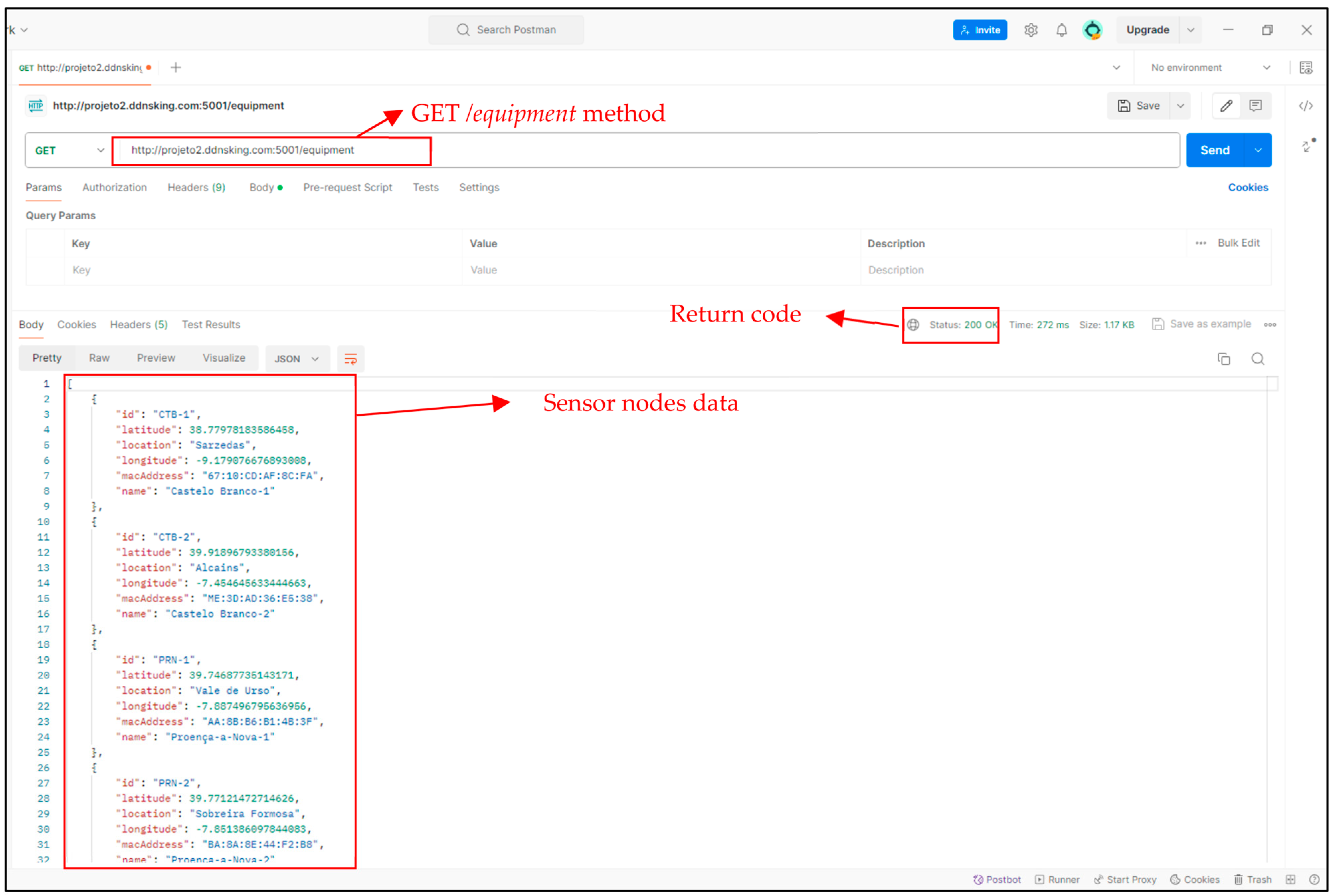
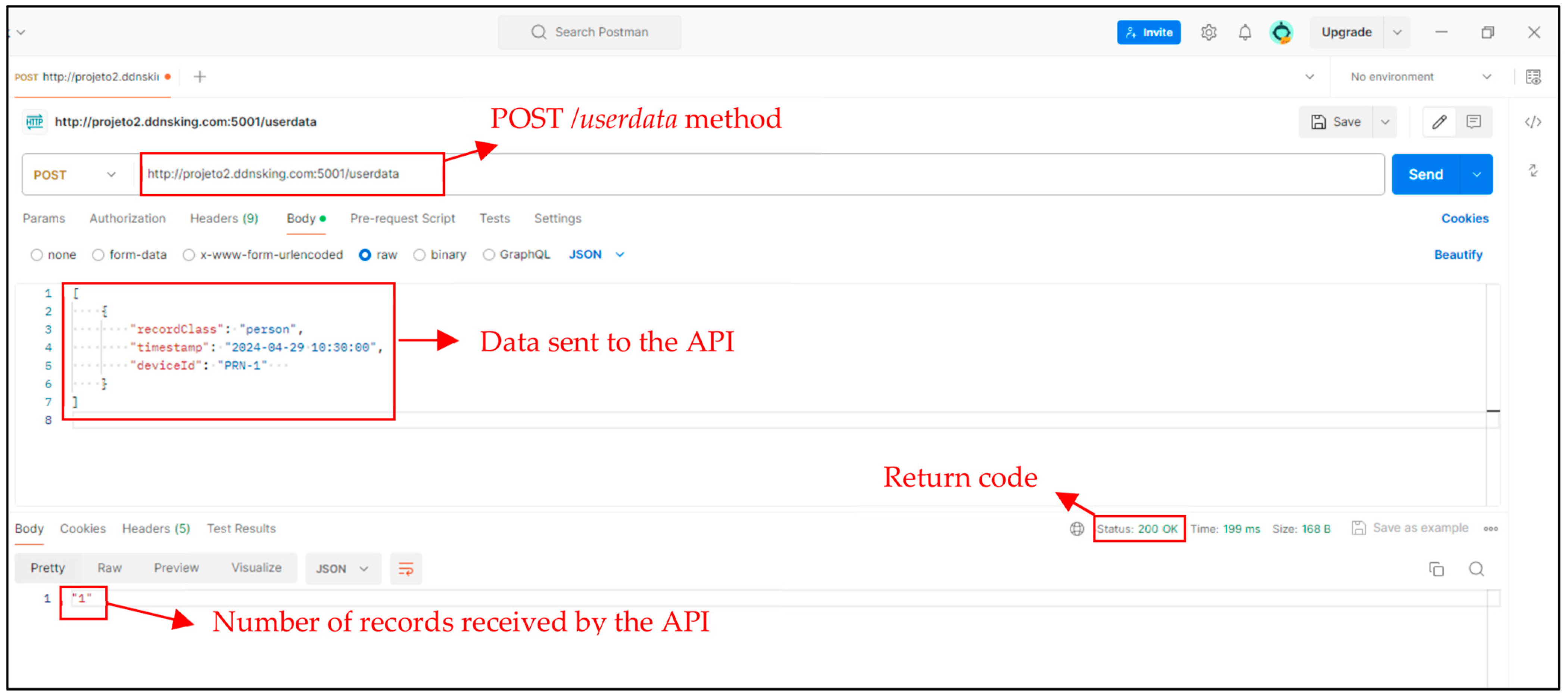
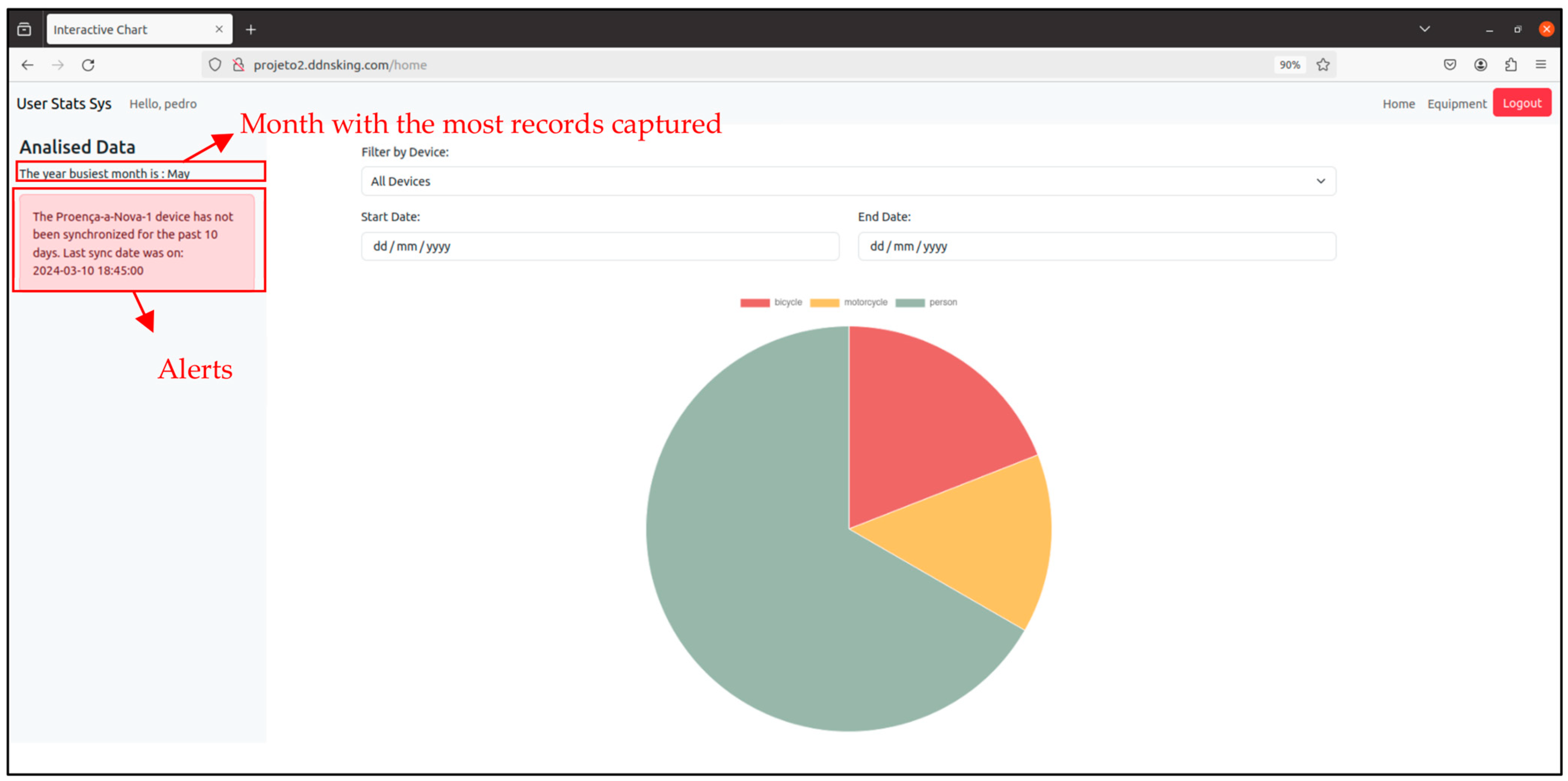
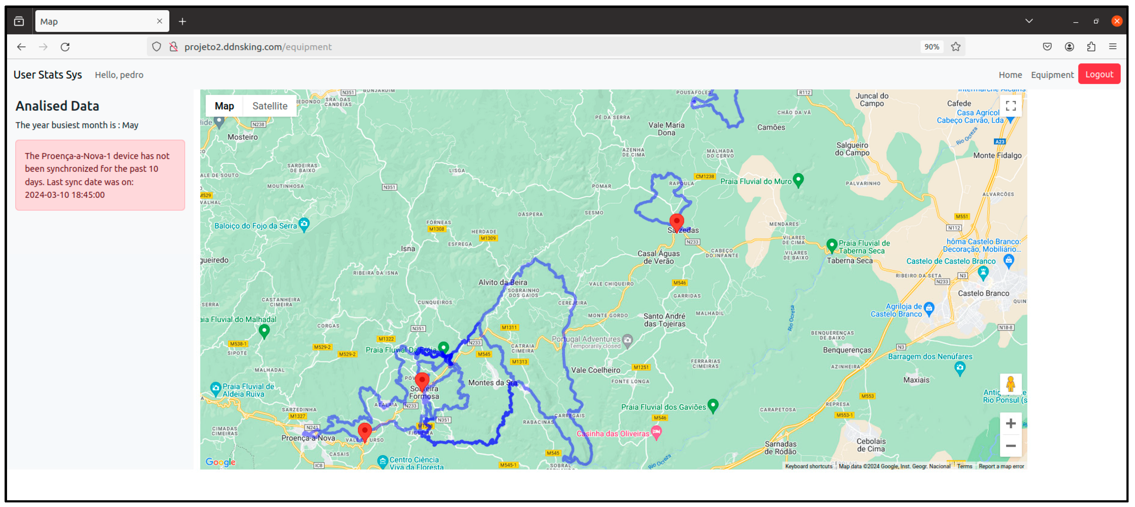
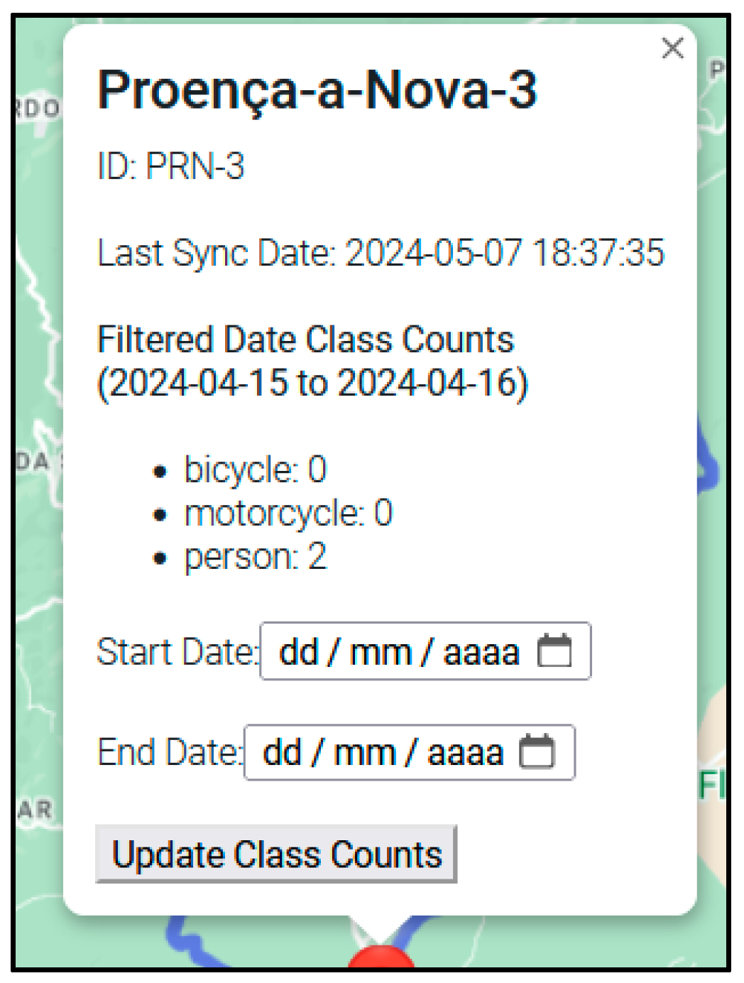
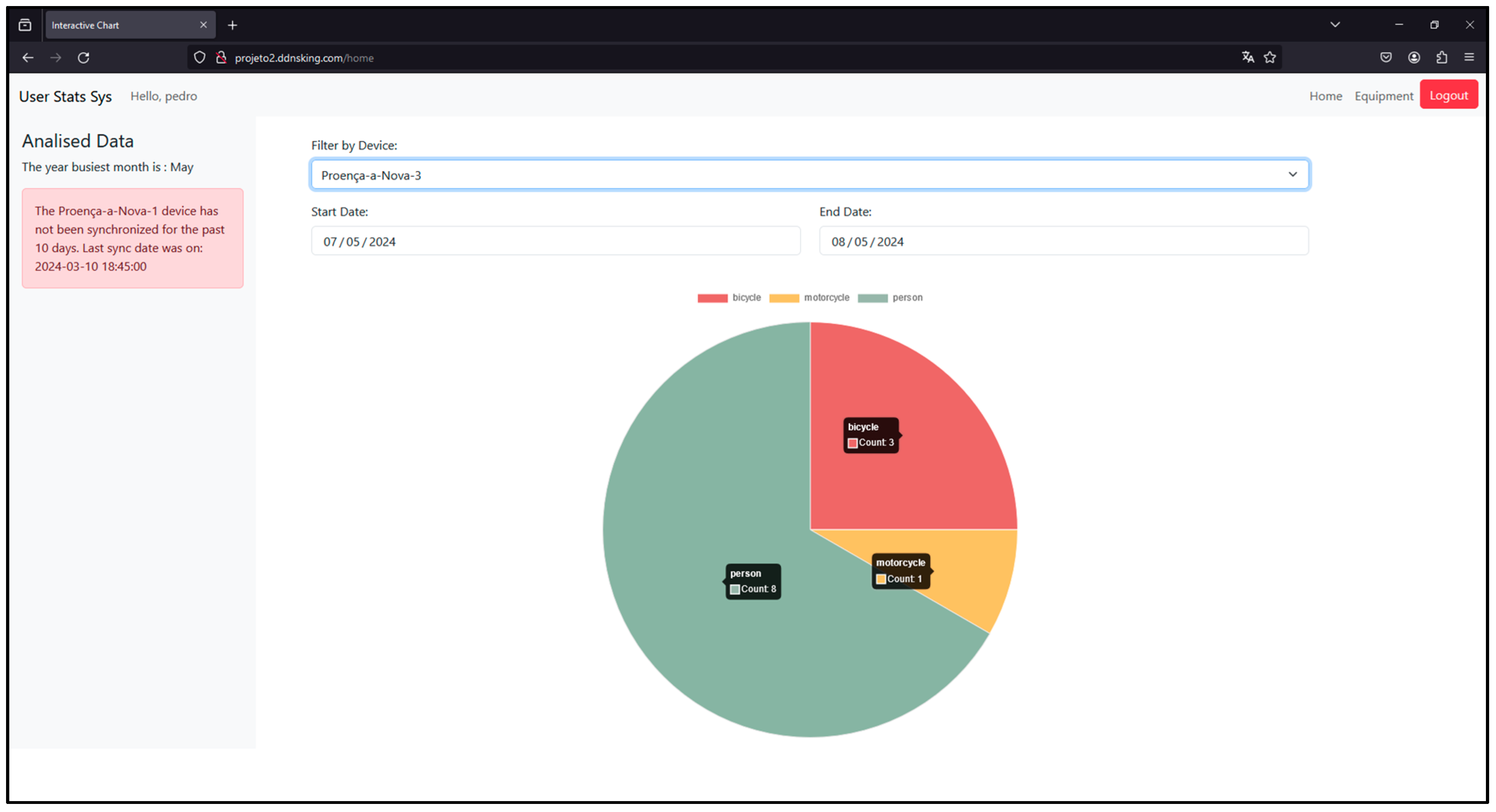
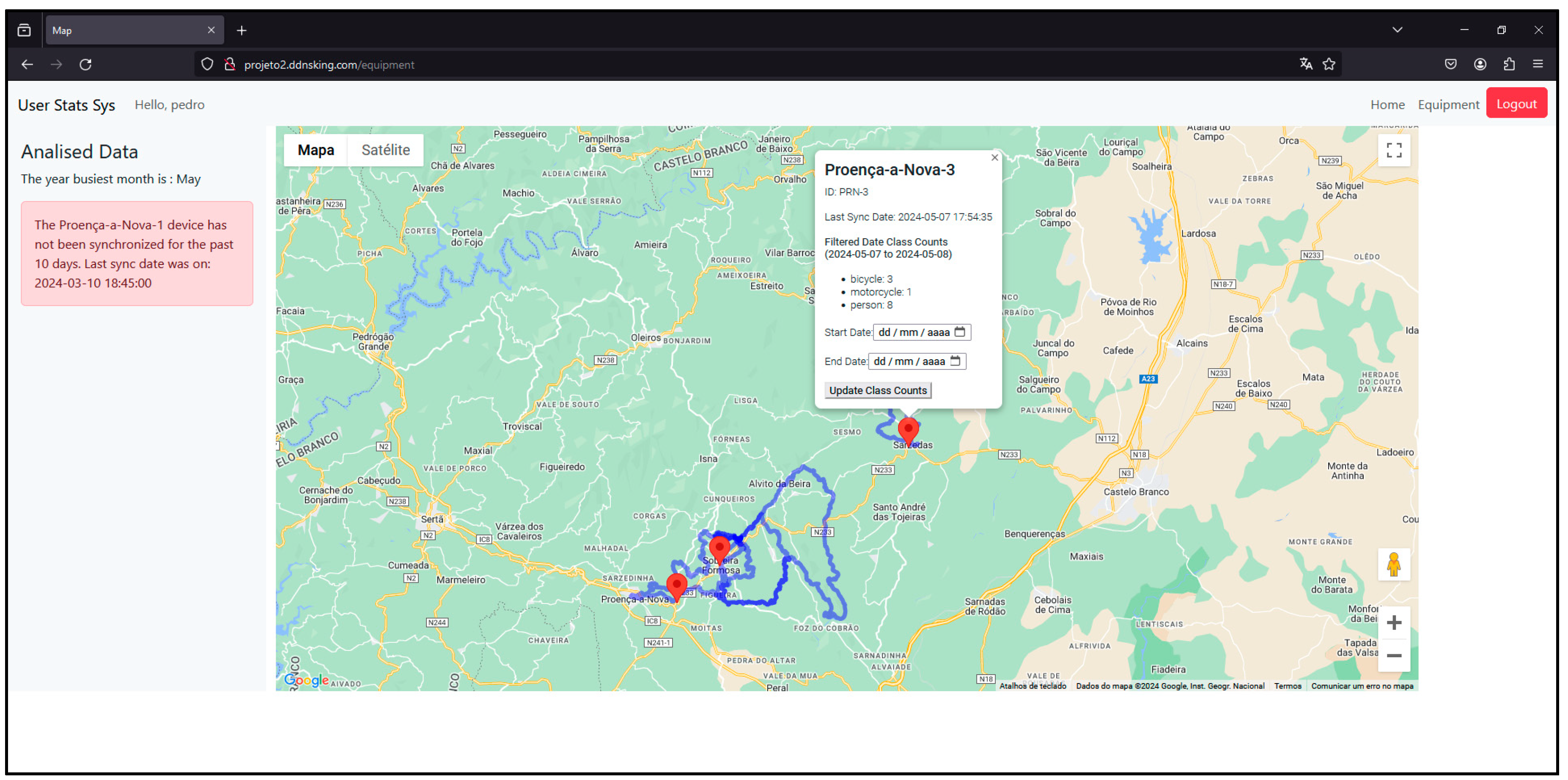
2.3.5. Application Server
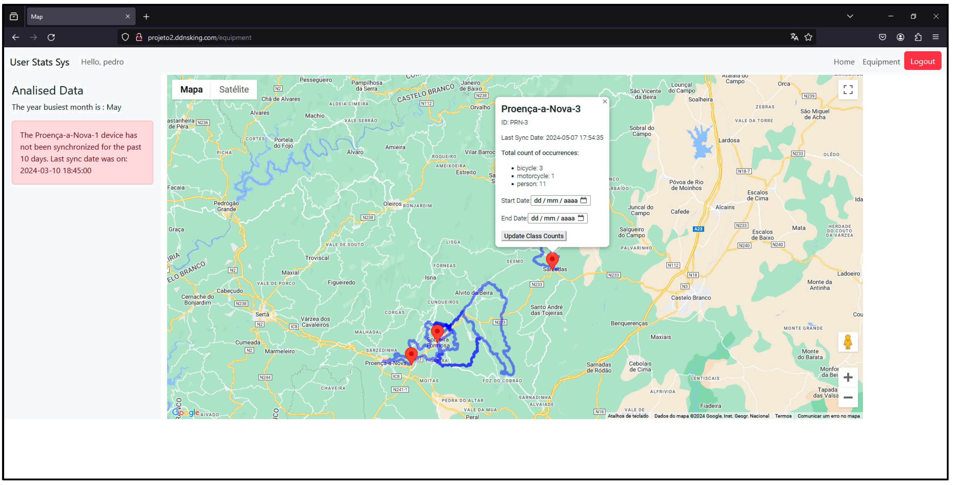
 on the map represents a sensor node. If you click on it, an information window will appear showing the name, id and counts of the different types of users it has detected since it has been active (Figure 34).
3. Testing and Validation
4. Conclusions and Future Work
Author Contributions
Funding
Institutional Review Board Statement
Informed Consent Statement
Data Availability Statement
Conflicts of Interest
References
- Federação de Campismo e Montanhismo de Portugal. Regulamento de Homologação De Percursos; Federação de Campismo e Montanhismo de Portugal: Lisboa, Portugal, 2006. [Google Scholar]
- Saos Sinalização. Available online: http://www.solasrotas.org/2008/09/sinalizao.html (accessed on 9 December 2023).
- Carvalho, P. Pedestrianismo e Percursos Pedestres. Cad. De Geogr. 2009, 28/29, 193–204. [Google Scholar]
- Federação de Campismo e Montanhismo de Portugal Site Oficial Da FCMP. Available online: https://www.fcmportugal.com/ (accessed on 16 January 2024).
- Federação de Campismo e Montanhismo de Portugal Site Oficial Da FCMP-Percursos Pedestres. Available online: https://www.fcmportugal.com/percursos-pedestres/ (accessed on 9 December 2023).
- Rails to Trails Conservancy Trail User Surveys and Counting. Available online: https://www.railstotrails.org/trail-building-toolbox/trail-user-surveys-and-counting/ (accessed on 18 May 2024).
- Lawson, M. Innovative New Ways to Count Outdoor Recreation: Using Data from Cell Phones, Fitness Trackers, Social Media, and Other Novel Data Sources; Headwaters Econ: Bozeman, MT, USA, 2021. [Google Scholar]
- Miguel, J.; Mendonça, P.; Quelhas, A.; Caldeira, J.M.L.P.; Soares, V.N.G.J. Using Computer Vision to Collect Information on Cycling and Hiking Trails Users. Future Internet 2024, 16, 104. [Google Scholar] [CrossRef]
- Adarsh, P.; Rathi, P.; Kumar, M. YOLO V3-Tiny: Object Detection and Recognition Using Stage Improved Model. In Proceedings of the 2020 6th International Conference on Advanced Computing & Communication Systems (ICACCS), Coimbatore, India, 6 March 2020; pp. 687–694. [Google Scholar]
- Sandler, M.; Howard, A.; Zhu, M.; Zhmoginov, A.; Chen, L.-C. MobileNetV2: Inverted Residuals and Linear Bottlenecks. In Proceedings of the IEEE Conference on Computer Vision and Pattern Recognition (CVPR), Salt Lake City, UT, USA, 18–23 June 2018; pp. 4510–4520. [Google Scholar]
- Wu, H.; Xin, M.; Fang, W.; Hu, H.M.; Hu, Z. Multi-Level Feature Network with Multi-Loss for Person Re-Identification. IEEE Access 2019, 7, 91052–91062. [Google Scholar] [CrossRef]
- Rodrigues, J.J.P.C.; Soares, V.N.G.J. Cooperation in DTN-Based Network Architectures. In Cooperative Networking; John Wiley & Sons, Ltd.: Hoboken, NJ, USA, 2011; pp. 101–115. [Google Scholar]
- Rodrigues, J.J.P.C.; Soares, V.N.G.J. An Introduction to Delay and Disruption-Tolerant Networks (DTNs). In Advances in Delay-Tolerant Networks (DTNs): Architecture and Enhanced Performance; Woodhead Publishing: Thorston, UK, 2014; pp. 1–21. [Google Scholar]
- Cerf, V.; Burleigh, S.; Hooke, A.; Torgerson, L.; Durst, R.; Scott, K.; Fall, K.; Weiss, H. Delay-Tolerant Networking Architecture. 2007. Available online: https://www.rfc-editor.org/info/rfc4838 (accessed on 30 April 2024).
- Videira, J.; Gaspar, P.D.; Soares, V.N.G.J.; Caldeira, J.M.L.P. A Mobile Application for Detecting and Monitoring the Development Stages of Wild Flowers and Plants. Informatica 2024, 48, 5645. [Google Scholar] [CrossRef]
- Videira, J.; Gaspar, P.D.; de Jesus Soares, V.N.d.G.; Caldeira, J.M.L.P. Detecting and Monitoring the Development Stages of Wild Flowers and Plants Using Computer Vision: Approaches, Challenges and Opportunities. Int. J. Adv. Intell. Inform. 2023, 9, 347–362. [Google Scholar] [CrossRef]
- Rodrigues, J.J.P.C.; Soares, V.N.G.J.; Farahmand, F. Stationary Relay Nodes Deployment on Vehicular Opportunistic Networks; Denko, M.K., Ed.; Auerbach Publications: Boca Raton, FL, USA, 2016; ISBN 97814-20088137. [Google Scholar]
- Soares, V.N.G.J.; Rodrigues, J.J.P.C.; Farahmand, F.; Denko, M. Exploiting Node Localization for Performance Improvement of Vehicular Delay-Tolerant Networks. In Proceedings of the IEEE International Conference on Communications, Cape Town, South Africa, 23 May 2010; pp. 1–5. [Google Scholar]
- Verma, M.; Singh, S.; Kaur, B. An Overview of Bluetooth Technology and Its Communication Applications. Int. J. Curr. Eng. Technol. 2015, 5, 1588–1592. [Google Scholar]
- Alecrim, E. Bluetooth: O Que é, Como Funciona e Versões. Available online: https://www.infowester.com/bluetooth.php (accessed on 30 April 2024).
- Collotta, M.; Pau, G.; Talty, T.; Tonguz, O.K. Bluetooth 5: A Concrete Step Forward toward the IoT. IEEE Commun. Mag. 2018, 56, 125–131. [Google Scholar] [CrossRef]
- He, N. Bluetooth VS WiFi VS Zigbee: Which Wireless Technology Is Better. Available online: https://www.mokosmart.com/bluetooth-vs-wifi-vs-zigbee-which-is-better/ (accessed on 13 May 2024).
- Putra, G.D.; Pratama, A.R.; Lazovik, A.; Aiello, M. Comparison of Energy Consumption in Wi-Fi and Bluetooth Communication in a Smart Building. In Proceedings of the 2017 IEEE 7th Annual Computing and Communication Workshop and Conference, CCWC 2017, Las Vegas, NV, USA, 9–11 January 2017. [Google Scholar]
- Spyropoulos, T.; Psounis, K.; Raghavendra, C.S. Spray and Wait: An Efficient Routing Scheme for Intermittently Connected Mobile Networks. In WDTN ’05: Proceedings of the ACM SIGCOMM Workshop on Delay-Tolerant Networking, Philadelphia, PA, USA, 22 August 2005; Association for Computing Machinery: New York, NY, USA; pp. 252–259.
- Soares, V.N.G.J.; Rodrigues, J.J.P.C.; Dias, J.A.; Isento, J.N. Performance Analysis of Routing Protocols for Vehicular Delay-Tolerant Networks. In Proceedings of the SoftCOM, 20th International Conference on Software, Telecommunications and Computer Networks, Split, Croatia, 11–13 September 2012. [Google Scholar]
- Raspberry Pi Raspberry Pi 4 Model B. Available online: https://www.raspberrypi.com/products/raspberry-pi-4-model-b/ (accessed on 29 April 2024).
- Raspberry Pi Raspberry Pi Camera Module 3. Available online: https://www.raspberrypi.com/products/camera-module-3/ (accessed on 29 April 2024).
- Shehab, M.A.; Al-Gizi, A.; Swadi, S.M. Efficient Real-Time Object Detection Based on Convolutional Neural Network. In Proceedings of the 2021 International Conference on Applied and Theoretical Electricity, ICATE 2021-Proceedings, Craiova, Romania, 27–29 May 2021. [Google Scholar]
- Xu, W.; Li, W.; Wang, L. Research on Image Recognition Methods Based on Deep Learning. Appl. Math. Nonlinear Sci. 2024, 9, 1–14. [Google Scholar] [CrossRef]
- Bhatt, D.; Patel, C.; Talsania, H.; Patel, J.; Vaghela, R.; Pandya, S.; Modi, K.; Ghayvat, H. CNN Variants for Computer Vision: History, Architecture, Application, Challenges and Future Scope. Electronics 2021, 10, 2470. [Google Scholar] [CrossRef]
- Barbosa, G.; Bezerra, G.M.; de Medeiros, D.S.; Andreoni Lopez, M.; Mattos, D. Segurança Em Redes 5G: Oportunidades e Desafios Em Detecção de Anomalias e Predição de Tráfego Baseadas Em Aprendizado de Máquina. In Proceedings of the XXI Simpósio Brasileiro em Segurança da Informação e de Sistemas Computacionais (SBSeg 2021), Belém, Brazil, 4–7 October 2021; pp. 164–165. [Google Scholar] [CrossRef]
- Poloni, K. Redes Neurais Convolucionais. Available online: https://medium.com/itau-data/redes-neurais-convolucionais-2206a089c715 (accessed on 1 November 2023).
- Archana, V.; Kalaiselvi, S.; Thamaraiselvi, D.; Gomathi, V.; Sowmiya, R. A Novel Object Detection Framework Using Convolutional Neural Networks (CNN) and RetinaNet. In Proceedings of the International Conference on Automation, Computing and Renewable Systems, ICACRS 2022-Proceedings, Pudukkottai, India, 13–15 December 2022; pp. 1070–1074. [Google Scholar]
- Carranza-García, M.; Torres-Mateo, J.; Lara-Benítez, P.; García-Gutiérrez, J. On the Performance of One-Stage and Two-Stage Object Detectors in Autonomous Vehicles Using Camera Data. Remote Sens. 2020, 13, 89. [Google Scholar] [CrossRef]
- Zhou, L.; Lin, T.; Knoll, A. Fast and Accurate Object Detection on Asymmetrical Receptive Field. arXiv 2023, arXiv:2303.08995. [Google Scholar]
- Thakur, N. A Detailed Introduction to Two Stage Object Detectors. Available online: https://namrata-thakur893.medium.com/a-detailed-introduction-to-two-stage-object-detectors-d4ba0c06b14e (accessed on 23 December 2023).
- Redmon, J.; Farhadi, A. YOLOv3: An Incremental Improvement. arXiv 2018, arXiv:1804.02767. [Google Scholar]
- Koteswararao, M.; Karthikeyan, P.R. Comparative Analysis of YOLOv3-320 and YOLOv3-Tiny for the Optimised Real-Time Object Detection System. In Proceedings of the 3rd International Conference on Intelligent Engineering and Management, ICIEM 2022, London, UK, 27–29 April 2022; pp. 495–500. [Google Scholar]
- Khokhlov, I.; Davydenko, E.; Osokin, I.; Ryakin, I.; Babaev, A.; Litvinenko, V.; Gorbachev, R. Tiny-YOLO Object Detection Supplemented with Geometrical Data. In Proceedings of the IEEE Vehicular Technology Conference, Antwerp, Belgium, 1 May 2020. [Google Scholar]
- Chen, S.; Lin, W. Embedded System Real-Time Vehicle Detection Based on Improved YOLO Network. In Proceedings of the 2019 IEEE 3rd Advanced Information Management, Communicates, Electronic and Automation Control Conference, IMCEC 2019, Chongqing, China, 1 October 2019; pp. 1400–1403. [Google Scholar]
- Miguel, J.; Mendonça, P. Person, Bicycle and Motorcyle Dataset. Available online: https://universe.roboflow.com/projeto-gfvuy/person-bicycle-motorcyle/model/7 (accessed on 26 January 2024).
- Google Colab. Available online: https://colab.google/ (accessed on 22 December 2023).
- Roboflow, Inc. Roboflow Website. Available online: https://roboflow.com/ (accessed on 22 November 2023).
- Roboflow Notebook-Train Yolov4 Tiny Object Detection On Custom Data. Available online: https://github.com/roboflow/notebooks/blob/main/notebooks/train-yolov4-tiny-object-detection-on-custom-data.ipynb (accessed on 23 December 2023).
- NVIDIA NVIDIA CUDA Compiler Driver. Available online: https://docs.nvidia.com/cuda/cuda-compiler-driver-nvcc/index.html (accessed on 23 December 2023).
- Darknet Darknet: Open Source Neural Networks in C. Available online: https://pjreddie.com/darknet/ (accessed on 23 December 2023).
- Charette, S. Programming Comments-Darknet FAQ. Available online: https://www.ccoderun.ca/programming/darknet_faq/ (accessed on 28 January 2024).
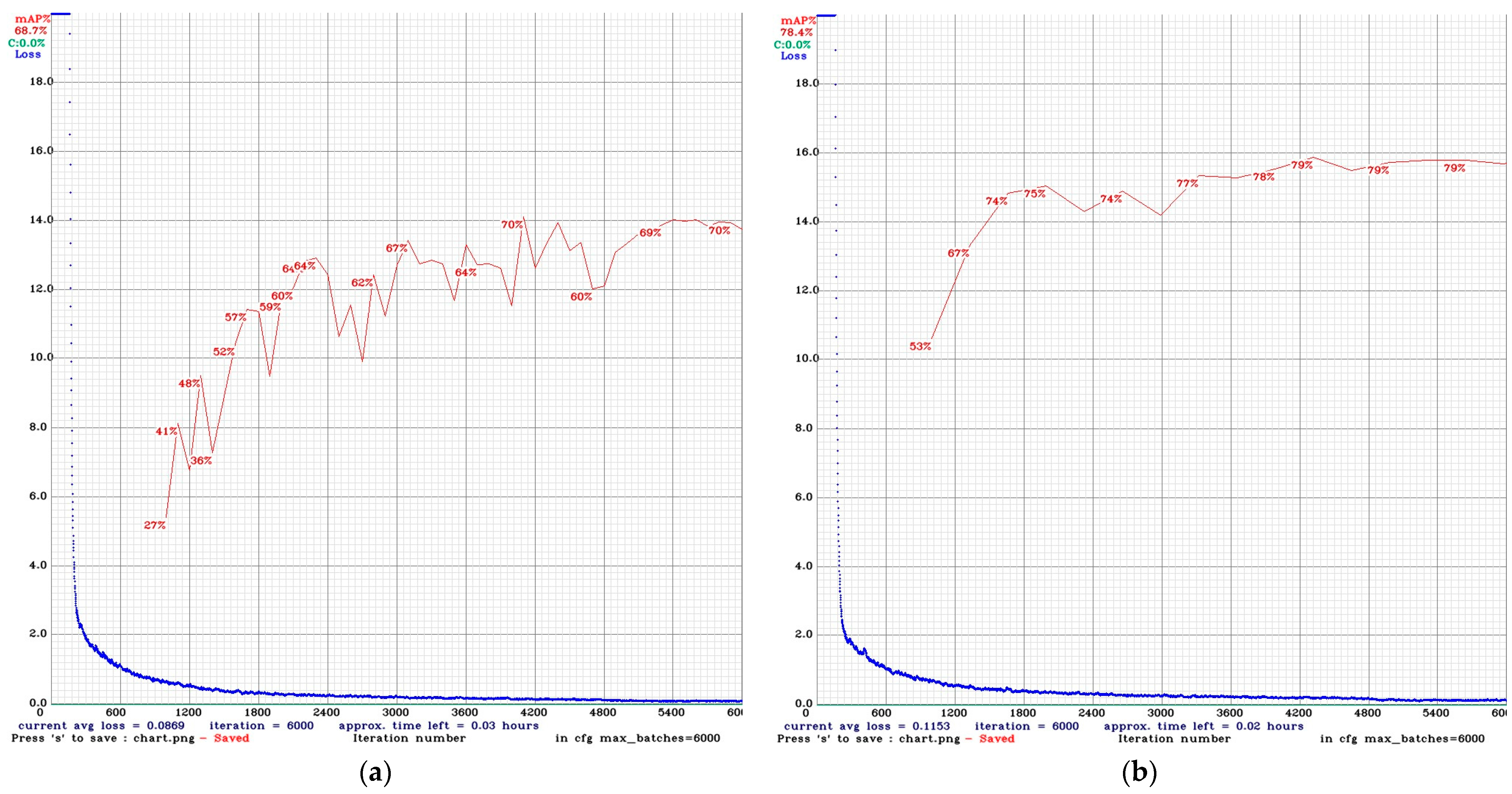
- Lakera Average Precision. Available online: https://www.lakera.ai/ml-glossary/average-precision (accessed on 17 January 2024).
- btd Performance Insights: Train Loss vs. Test Loss in Machine Learning Models|Medium. Available online: https://baotramduong.medium.com/machine-learning-train-loss-vs-test-loss-735ccd713291 (accessed on 14 May 2024).
- Raspberry Raspberry Pi OS (Legacy) Lite. Available online: https://downloads.raspberrypi.com/raspios_oldstable_lite_arm64/images/raspios_oldstable_lite_arm64-2024-03-12/2024-03-12-raspios-bullseye-arm64-lite.img.xz (accessed on 9 May 2024).
- MariaDB Foundation MariaDB DBMS. Available online: https://mariadb.org/ (accessed on 12 June 2024).
- Certificadora, V. Criptografia Simétrica e Assimétrica: Qual é a Diferença Entre Elas? Available online: https://blog.validcertificadora.com.br/criptografia-simetrica-e-assimetrica-qual-e-diferenca-entre-elas/ (accessed on 1 May 2024).
- Milanov, E. The RSA Algorithm; RSA laboratories: Burlington, MA, USA, 2009. [Google Scholar]
- Evans, D.L.; Brown, K.H. Advanced Encryption Standard (AES); National Institute of Standards and Technology: Gaithersburg, MD, USA, 2001. [Google Scholar]
- Filatov, I. Hybrid Encryption in Python. Available online: https://medium.com/@igorfilatov/hybrid-encryption-in-python-3e408c73970c (accessed on 1 May 2024).
- Bluetooth® Technology RFCOMM. Available online: https://www.bluetooth.com/specifications/specs/rfcomm-1-1/ (accessed on 4 May 2024).
- Android Developers BluetoothDevice. Available online: https://developer.android.com/reference/android/bluetooth/BluetoothDevice (accessed on 4 May 2024).
- MDN BluetoothUUID. Available online: https://developer.mozilla.org/en-US/docs/Web/API/BluetoothUUID (accessed on 1 May 2024).
- W3schools What Is JSON. Available online: https://www.w3schools.com/whatis/whatis_json.asp (accessed on 1 May 2024).
- Oracle Corporation Dev.Java: The Destination for Java Developers. Available online: https://dev.java/ (accessed on 30 April 2024).
- Google Download Android Studio & App Tools-Android Developers. Available online: https://developer.android.com/studio (accessed on 30 April 2024).
- Google Service|Android Developers. Available online: https://developer.android.com/reference/android/app/Service (accessed on 30 April 2024).
- Google Activity|Android Developers. Available online: https://developer.android.com/reference/android/app/Activity (accessed on 30 April 2024).
- Google Markers|Android Developers. Available online: https://developers.google.com/maps/documentation/android-sdk/marker#maps_android_markers_add_a_marker-java (accessed on 30 April 2024).
- Google Salvar Dados Usando o SQLite|Android Developers. Available online: https://developer.android.com/training/data-storage/sqlite?hl=pt-br (accessed on 9 May 2024).
- Oracle MySQL. Available online: https://www.mysql.com/ (accessed on 9 May 2024).
- Ubuntu 20.04.6 LTS (Focal Fossa). Available online: https://releases.ubuntu.com/20.04.6/?_ga=2.149898549.2084151835.1707729318-1126754318.1683186906 (accessed on 9 May 2024).
- Google KML Documentation Introduction|Keyhole Markup Language|Google for Developers. Available online: https://developers.google.com/kml/documentation (accessed on 2 May 2024).
- Google Keyhole Markup Language|Google for Developers. Available online: https://developers.google.com/kml (accessed on 2 May 2024).
- dassouki Gis-Loading a Local.Kml File Using Google Maps?-Stack Overflow. Available online: https://stackoverflow.com/questions/3514785/loading-a-local-kml-file-using-google-maps (accessed on 2 May 2024).
- ScaisEdge Google Maps-Unable to Access KML File for KML Layer|Stackoverflow. Available online: https://stackoverflow.com/questions/35851509/google-maps-unable-to-access-kml-file-for-kml-layer (accessed on 16 May 2024).
- nrabinowitz Google Maps API and KML File LocalHost Development Options|Stackoverflow. Available online: https://stackoverflow.com/questions/6092110/google-maps-api-and-kml-file-localhost-development-options (accessed on 16 May 2024).
- Burke, K.; Conroy, K.; Horn, R.; Stratton, F.; Binet, G. Flask-RESTful—Flask-RESTful 0.3.10 Documentation. Available online: https://flask-restful.readthedocs.io/en/latest/ (accessed on 4 May 2024).
- Le Wagon O Que é Padrão MVC? Entenda Arquitetura de Softwares! Available online: https://blog.lewagon.com/pt-br/skills/o-que-e-padrao-mvc/ (accessed on 2 May 2024).
- Pallets Projects Flask. Available online: https://flask.palletsprojects.com/en/3.0.x/ (accessed on 2 May 2024).
- Google. Google for Developers-API Maps JavaScript. Available online: https://developers.google.com/maps/documentation/javascript/overview?hl=pt-br (accessed on 2 May 2024).
- Miguel, J.; Mendonça, P. Person,Bicycle,Motorcyle Dataset > Overview. Available online: https://app.roboflow.com/projeto-gfvuy/person-bicycle-motorcyle/overview (accessed on 24 May 2024).
- Termius Termius-SSH Platform for Mobile and Desktop. Available online: https://termius.com/ (accessed on 9 May 2024).


| Challenges | Hypotheses |
|---|---|
| (A1) When can data be deleted from the sensor node? | Create an attribute (i.e., threshold) to control the number of bridge nodes that carry the users count information. After a period of time. After the storage capacity is above a certain threshold. Specific event. A request from the infrastructure manager. |
| (A2) How can data be transmitted securely between the sensor node and the bridge node? | Data encryption. Mutual authentication between nodes. |
| (A3) Are all of the different types of bridge nodes able to receive the data transmitted by the node? | Will the speed of the bikes make it impossible to establish a connection and exchange data between the sensor and bridge nodes? Compatibility of the user’s smartphone (operating system, operating system version, Bluetooth version). |
| (A4) How can data transmission be ensured transparently, without the user having to interact with the application? | Automatic device detection. Background processes. |
| (A5) What happens if the sensor and bridge nodes disconnect in the middle of the transmission process? | Try reconnecting the devices and sending all of the information again. Attempt to reconnect the devices and resend the information that was not successfully sent. Timing a reconnection attempt. |
| No. of Training Images | No. of Validation Images | No. of Test Images | |
|---|---|---|---|
| Persons | 186 | 54 | 26 |
| Bicycles | 260 | 78 | 32 |
| Motorcycles | 323 | 92 | 45 |
| Total | 769 | 224 | 103 |
Disclaimer/Publisher’s Note: The statements, opinions and data contained in all publications are solely those of the individual author(s) and contributor(s) and not of MDPI and/or the editor(s). MDPI and/or the editor(s) disclaim responsibility for any injury to people or property resulting from any ideas, methods, instructions or products referred to in the content. |
© 2024 by the authors. Licensee MDPI, Basel, Switzerland. This article is an open access article distributed under the terms and conditions of the Creative Commons Attribution (CC BY) license (https://creativecommons.org/licenses/by/4.0/).
Share and Cite
Miguel, J.; Mendonça, P.; Quelhas, A.; Caldeira, J.M.L.P.; Soares, V.N.G.J. The Development of a Prototype Solution for Collecting Information on Cycling and Hiking Trail Users. Information 2024, 15, 389. https://doi.org/10.3390/info15070389
Miguel J, Mendonça P, Quelhas A, Caldeira JMLP, Soares VNGJ. The Development of a Prototype Solution for Collecting Information on Cycling and Hiking Trail Users. Information. 2024; 15(7):389. https://doi.org/10.3390/info15070389
Chicago/Turabian StyleMiguel, Joaquim, Pedro Mendonça, Agnelo Quelhas, João M. L. P. Caldeira, and Vasco N. G. J. Soares. 2024. "The Development of a Prototype Solution for Collecting Information on Cycling and Hiking Trail Users" Information 15, no. 7: 389. https://doi.org/10.3390/info15070389