Article

Semi-Supervised Learning for Multi-View Data Classification and Visualization

1
Faculty of Computer Engineering, Shahid Rajaee Teacher Training University, Tehran 16785163, Iran
2
Faculty of Computer Engineering, University of the Basque Country, 20018 San Sebastian, Spain
3
IKERBASQUE, Basque Foundation for Science, 48009 Bilbao, Spain
*
Author to whom correspondence should be addressed.
Information 2024, 15(7), 421; https://doi.org/10.3390/info15070421
Submission received: 26 March 2024 / Revised: 27 June 2024 / Accepted: 12 July 2024 / Published: 22 July 2024
(This article belongs to the Special Issue Interactive Visualizations: Design, Technologies and Applications)

Abstract

:
Data visualization has several advantages, such as representing vast amounts of data and visually demonstrating patterns within it. Manifold learning methods help us estimate lower-dimensional representations of data, thereby enabling more effective visualizations. In data analysis, relying on a single view can often lead to misleading conclusions due to its limited perspective. Hence, leveraging multiple views simultaneously and interactively can mitigate this risk and enhance performance by exploiting diverse information sources. Additionally, incorporating different views concurrently during the graph construction process using interactive visualization approach has improved overall performance. In this paper, we introduce a novel algorithm for joint consistent graph construction and label estimation. Our method simultaneously constructs a unified graph and predicts the labels of unlabeled samples. Furthermore, the proposed approach estimates a projection matrix that enables the prediction of labels for unseen samples. Moreover, it incorporates the information in the label space to further enhance the accuracy. In addition, it merges the information in different views along with the labels to construct a consensus graph. Experimental results conducted on various image databases demonstrate the superiority of our fusion approach compared to using a single view or other fusion algorithms. This highlights the effectiveness of leveraging multiple views and simultaneously constructing a unified graph for improved performance in data classification and visualization tasks in semi-supervised contexts.

1. Introduction

The reason for the success of data visualization is that it can give us a rapid insight into the data and their relations [1]. In real life, we often face data that have a lot of dimensions; hence, it is challenging to visualize the data. One possible solution among others is to transform the data into another medium that enables effective visualization. Two possible options are using graphs and reducing the dimensions. Graphs are useful tools that help us to determine the relation between the samples and visualize this relationship. On the other hand, dimensionality reduction and embedding calculation methods enable the visualization of data by extracting lower and informative dimensions from data, making it easier to visualize and analyze complex data [2]. For instance, a large number of features need to be mapped into a smaller number that fit the suitable and effective visualization criteria, e.g., if 100 features can be effectively mapped to 3 features, the data can be visualized in a 3D space. Additionally for reducing the number of features, interactivity can be referred to as an instrument to keep data at a low dimensional level allowing it to zoom into other levels of data when required.
One popular embedding calculation method used in data visualization is t-Distributed Stochastic Neighbor Embedding (t-SNE) [3]. t-SNE is a nonlinear dimensionality reduction technique particularly useful for visualizing high-dimensional datasets. It converts data similarities into joint probabilities and then optimizes the placement of points in a lower-dimensional space to approximate the input probabilities. UMAP (Uniform Manifold Approximation and Projection) [4] is a nonparametric graph-based dimensionality reduction algorithm that applied Riemannian geometry and algebraic topology to find low-dimensional embeddings of structured data. The authors of [5] extended UMAP to a parametric optimization over neural network weights, learning a parametric relationship between data and embedding. The method was adopted for representation and semi-supervised learning.
The rapid growth of data, mostly unlabeled and few labeled, causes attraction toward semi-supervised learning methods since they can benefit from the information from both labeled and unlabeled samples [6,7]. Graph-based learning methods are a widely used method that can benefit from the labeled and unlabeled samples simultaneously. Graph-based semi-supervised learning algorithms use an affinity graph to transfer the label of the labeled data to the unlabeled data. The affinity graph represents how close the samples are to each other, so its construction is important and has a crucial impact on the results.
While most learning algorithms focus on using a single view or descriptor [8], using multiple views can improve the performance of learning tasks [9,10,11,12,13]. One of the main problems with using multiple descriptors is the fusion of the available information in the views.
Recently, the use of multiple descriptors to construct graphs has attracted the attention of researchers [14,15,16]. The main goal in graph-based multi-view learning is to use the affinity graph(s) to utilize and merge the available information in different views. One of the most common solutions in graph-based multi-view learning is to take multiple pre-constructed graphs and merge them [17,18,19].
The main difference in these algorithms is how the graphs are merged to construct a unified graph. While several fusion algorithms exist, in [18], the authors constructed several similarity matrices using the Gaussian kernel as the edge weighting method and then adopted linear summation of the normalized similarity matrices. In another study, the authors of [20] proposed an adaptive weight assignment where the weight for each view is calculated using a function of label smoothness assumption. In [17], the authors considered that some of the views might be noisy and contain misleading information, so it is better to exclude them from the fusion process by assigning them a very small weight. They achieve their goal by applying sparsity constraints to the weights. In [19], the authors proposed an algorithm that iteratively updates the similarity matrix corresponding to each of the descriptors by fusing the similarity matrix of other views and the similarity of the neighbors of each view.
In addition to using descriptors extracted from the data, some algorithms try to also extract information from the label of samples and create the affinity matrix by looking at the similarity between labels [9,21]. Hence, using the labels along with feature descriptors as a source of information for graph construction can lead to a graph with richer edges.
Recent multi-view methods focus on directly constructing a unified graph by fusing the information in the feature spaces [22]. These methods do not adopt pre-constructed graphs as inputs. The direct construction of the graph from the features eliminates the different choices for graph construction and can lead to graphs with fewer erroneous edges.
Since graph construction is an intermediate step in Graph-based Label Propagation methods, some algorithms treat graph construction and the post-graph learning task (e.g., label propagation) as two separate tasks [9,19]. In these methods, an affinity matrix is constructed in the first step (or the affinity matrices obtained from different descriptors are merged to obtain one graph), and then the fused graph is adopted to estimate the label of unknown samples. However, this is not the best choice because the label of the samples may also affect the affinity matrix [21]; hence, constructing the graph and propagating the labels should not be treated as separate tasks.
One of the important issues in the applicability of semi-supervised methods is how they treat the samples not presented in the learning process. The works in [23,24] are transductive methods, meaning that they can only estimate the labels in the training set. In these algorithms, for new unseen samples, the algorithm has to start from scratch and one has to repeat the whole learning process. On the other hand, inductive methods estimate a mapping function from the feature space to the label space [25]. Using the mapping function, one can directly estimate the label of unseen samples via the projection matrix without repeating the learning process.
Based on what is explained above, in this article, we propose a unified criterion that has the following advantages.
  • It benefits from multiple descriptors for each sample. This can improve the unified graph estimation, which can well represent the relationship between nodes.
  • It automatically fuses the information of different views.
  • It not only uses the information in the feature space but also uses the available information in the label space.
  • It does not require pre-constructed graphs based on individual views but can construct a single graph by considering the information from different views.
  • The process of constructing the affinity graph and propagating the labels is simultaneously carried out in a single framework.
  • It estimates a linear projection function to estimate the label of unseen samples.
The rest of this paper is organized as follows: Section 2 surveys some basic assumptions about graph-based semi-supervised learning and reviews some of the previous works in this area. Section 3 presents our proposed algorithm. In Section 4, we report the experimental results on public databases. Finally, Section 5 concludes the paper.

2. Related Work

2.1. Notations

Let X R d × N denote the data matrix where d represents the dimensionality of each sample and N is the number of samples. Without loss of generality, we consider that the data are relocated such that the first l samples are labeled ones and the rest of the samples (from l + 1 to l + u ) are unlabeled. Moreover, Y = [ Y l , Y u ] = [ y 1 ; y 2 ; . . . . ; y l ; y l + 1 ; . . . ; y l + u ] R N × C where C is the number of classes of the corresponding binary labels. For the labeled sample x i that belongs to the c t h class, we have y i c = 1 and zero for other elements. Moreover, for unlabeled samples, the Y u matrix (the label matrix of unlabeled samples) is a zero matrix. Similarly, we have the soft label matrix F = [ f 1 ; f 2 ; . . . . ; f N ] R N × C , where F i c shows the probability that sample x i belonging to the c t h class.
In addition, consider an affinity graph as G = { X , W } , where X is the set of nodes (i.e., the data matrix) and W is the symmetric affinity matrix, where w i j denotes the similarity between nodes x i and x j . Also, the Laplacian matrix is defined as L = D W , where D is a diagonal matrix with D i i = j = 1 N W i j and zero otherwise.

2.2. Gaussian Field and Harmonic Functions [26]

The cluster hypothesis, which is one of the basic assumptions in label propagation, assumes that the nodes that are close to each other in the feature space should have similar labels (i.e., their corresponding label vectors should be close to each other). Mathematically, it can be written as
min F i , j = 1 N | | f i f j | | 2   W i j = min F   T r ( F T   L   F )
where T r ( . ) indicates the trace of a matrix. For the pair of samples x i and x j with corresponding soft labels f i and f j , respectively, the similarity between the pair of nodes is coded in W i j . It is worth noting that W i j can be estimated using any similarity function like Cosine. Equation (1) asserts that, if W i j is high (the pair of samples are similar), then the corresponding soft labels should be similar (i.e., the difference between them should be small). The solution of the objective function of Equation (1) that gives the label of unlabeled samples (i.e., f u ) is
f u = ( D u u W u u ) 1 W u l f l
where W u u is the subgraph of the W matrix that shows the similarity between the unlabeled samples and D u u is its corresponding Laplacian matrix, and W u l is the subgraph of the W matrix that shows the similarity between the unlabeled and labeled samples and f l contains the label of labeled samples [26].

2.3. Local and Global Consistency [27]

A second notion that can be adopted is that the prediction of the samples should be such that the predicted label of the labeled samples is close to their true label. This is called label fitness and can be written in mathematical terms as follows.
min F i = 1 l | | f i y i | | 2 = min F T r   ( F Y ) T   U   ( F Y ) .
where the diagonal matrix U is U i i = 0 for the unlabeled samples and U i i 0 for the labeled samples.
By adding Equation (3) to Equation (1), one can define a new minimization function (known as the Local and Global Consistency [27]) as
min F i , j = 1 N | | 1 D i i   f i 1 D j j   f j | | 2   W i j + μ i = 1 l | | f i y i | | 2
where μ is the balance parameter. The first term that enforces close samples to have similar labels is local and is based on the assumption that nearby points are likely to have the same label. The second term that enforces samples in a cluster or class to have similar labels is global and is based on the assumption that points on the same structure (typically referred to as a cluster or a manifold) are likely to have the same label.
Following some mathematical operations, the problem of Equation (4) can be rewritten as
min F T r   ( F T   L   F ) + T r   ( F Y ) T   U   ( F Y )
where U is a diagonal matrix with U i i = μ for the labeled samples.

2.4. Review on Flexible Manifold Embedding [25]

One of the drawbacks of the works described in [26,27] is that they can only deal with unlabeled samples and predict their label. When a new sample arrives, one has to construct a new graph using the new sample and solve the minimization function.
The Flexible Manifold Embedding (FME) method [25] solves this problem by adding a projection matrix calculation to the minimization function of the LGC in Equation (5). The projection matrix is computed to provide label estimation of an arbitrary sample via a linear mapping. In other words, the projection matrix defines a function to map data features to the label space. The objective function of the FME is
min F ,   Q ,   b T r   ( F T   L   F ) + T r   ( F Y ) T   U   ( F Y ) + μ   ( γ   | | X T Q + 1 b T F | | 2 + | | Q | | 2 )
The first term is called the label smoothness term (similar to the objective function of GRF in Equation (1)) which penalizes the pair of samples ( x i and x j ) with high similarity (high W i j ) having different labels. In other words, it enforces similar samples to have close (similar) label vectors. The second term represents the fitness of labels on labeled samples which penalizes the labeled samples when their true labels and predicted ones are different. In other words, it enforces the true label and predicted label of labeled samples to be similar. The third term is the error of label fitness of all samples adopting linear projection; it enforces the predicted label of each sample obtained via linear projection to be similar to its soft label value. The fourth term is the regularization of the projection matrix. μ and γ are two balance parameters that control the importance of the label estimation error and sparsity of the projection matrix, and | | . | | 2 declares the 2 norm of a matrix. Equation (6) has a closed-form solution as
Q = γ   [ γ   X H c X T + I ] 1 X H c F
b = 1 l + u [ F T 1 W T X 1 ]
F = ( U + L + μ   γ   H c μ   γ 2   M ) 1 U   Y
where M = X c T   X c   ( γ   X c T   X c + I ) 1 . X c and H c = I 1 l + u 1   1 T are the centered data matrix and the centering matrix, respectively. The mathematical proofs of Equations (7)–(9) are described in [25].

2.5. Data Smoothness Assumption

The data smoothness assumption states that two samples that are close to each other in the embedding space should also have similar labels. Since the similarity between nodes is encoded in the affinity matrix, it can be defined mathematically as follows:
min S 1 2 i , j = 1 N | | x i x j | | 2   P i j = min S T r   ( X   L   X T )
where the L matrix represents the Laplacian matrix of the graph P .

3. Proposed Method

3.1. Learning Model

By merging data smoothness in the FME framework; we propose a Joint Graph Construction and multi-view FME algorithm (JGC-MFME), which has two advantages. First, it helps us to estimate the affinity graphs directly, so there is no need to use a previously constructed graph. Second, it helps us use multiple sources of information to construct a graph that represents the relationship between samples. The proposed method also unifies the graph construction and classification into a single criterion.
To make the data smoothness term suitable for multi-view learning, we define it as
min S v = 1 V   i , j = 1 N | | x v i x v j | | 2   S i j = min S v = 1 V   T r ( X v   L   X v T )
where x v j represents the v t h view of the j t h sample and V denotes the number of views. It states that the unified similarity matrix should satisfy the data smoothness assumption in all views. As we explained before, to have a single similarity matrix when we have several views, one possible option is to calculate one affinity graph in each view that encodes the similarity between the pair of samples in that view and preserves the data smoothness assumption of that view. Then, for a unified graph, one can merge the calculated affinity matrices of different views. The second solution is to directly construct one affinity matrix such that it simultaneously preserves the smoothness assumption in all views. In other words, the similarity between each pair is calculated such that the smoothness assumption is minimized among all views.
The proposed criterion is constructed by inserting Equation (11) to the FME framework as follows:
min S , F , Q , b [ v = 1 V   T r ( X v   L   X v T ) + λ   T r ( F T   L   F ) + T r ( ( F Y ) T   U   ( F Y ) ) + γ   | | S | | 2   + μ   ( | | Q | | 2 + α   | | X c o n c T Q + 1 b T F | | 2 ) ] s . t .   0 S i j 1   j = 1 N S i j = 1
where S is the unified similarity matrix. By solving the above criteria, we obtain the unified similarity matrix, the soft label matrix, the projection matrix, and the bias vector, i.e., S , F , W , and b , respectively. It is worth noting that, since we have multiple descriptors, we concatenate the features of the descriptors to form the matrix X c o n c . As a result, the size of X c o n c becomes ( v = 1 V d v ) × N .
In the following, we explain the novelties of the proposed method from the objective function. As we can see, the first and second terms in Equation (12) show the presence of the data along with the labels in the objective function which shows that not only the features but also the labels affect the objective function. As mentioned before, this is one of the contributions of this article. Moreover, we observe that the consensus affinity graph (i.e., S ) is an unknown of the proposed method which shows that it is not a pre-constructed graph but an automatically estimated one. Moreover, the consensus affinity graph (i.e., S ) along with the labels (i.e., F ) is an output of the optimization function which shows that the proposed method simultaneously estimates these unknowns inside its objective function. Furthermore, the linear projection function is also an output of the proposed method which helps us to estimate the label of unseen samples without repeating the optimization process.

3.2. Optimization

In the following, we present an iterative alternating scheme to solve Equation (12).
Step1: Fix F , Q , and b , and update S . Since F , Q , and b are fixed, the problem in Equation (12) becomes:
min S           v = 1 V   T r   ( X v   L   X v T )   + λ   T r ( F T   L   F ) + γ   | | S | | 2 s . t .   0 S i j 1   j = 1 N S i j = 1
Denote d i j x = v = 1 V | | x i v x j v | | 2 2 and d i j f = | | f i f j | | 2 2 as the distance between nodes x i and x j in all views and the distance between their soft labels, respectively.
We rewrite Equation (13) as follows:
min S   i , j = 1 N S i j   ( d i j x + λ   d i j f ) + γ   | | S | | 2 2 = min S   i , j = 1 N [ S i j   d i j + γ   S i j 2 ] s . t .   0 S i j 1   j = 1 N S i j = 1
where d i j = d i j x + λ   d i j f .
The solution of Equation (14) can be obtained by the algorithm presented in [22].
Step 2: Fix S , and update Q , b , and F . Thus, since S is fixed, the problem of Equation (12) can be simplified as follows:
min F , Q , b   λ   T r ( F T   L   F )   + ( F Y )   U   ( F Y ) T + μ   ( | | Q | | 2 + α   | | X c o n c T Q + 1 b T F | | 2 )
This is nothing but the FME problem shown in Equation (6). Thus, the solution can be obtained using Equations (7)–(9).
It should be mentioned that one can estimate the label of a test sample via
f = x c o n c T   Q + 1 b T
where x c o n c is the concatenation of features of all views.
Apart from the class label obtained from the f vector, one can also use it for interactive visualization. One possible use of these visualizations is in active learning [28,29,30] and incremental learning, where labeled samples are incrementally added to a database. In these cases, users progressively increase the number of labeled samples and immediately visualize the data. Via visualization one can determine the samples that are close to the class border and, hence, are difficult to classify and cause misclassification. Consequently, the user can assign a label to those samples. In this way, it is unnecessary to set labels for all samples but only those in the class border which can cause misclassification.

4. Experimental Results

This section is dedicated to the comparison of the performance of the proposed method with that of several state-of-the-art algorithms. The algorithms that we adopt for comparison are FME with single view, FME with concatenating feature descriptors, SNF [19], SMGI [17], DGFLP [21], MLGC [18], and AMGL [31].

4.1. Databases

We use four image databases, namely PF01 [32], PIE [33], FERET [34], and MNIST [35], to evaluate the performance of the proposed method. PF01 contains 1819 images from 103 subjects with 17 images each. For the PIE database, we take a subset containing 1926 images from 68 subjects. In the FERET database, we use a subset with 1400 images of 200 subjects, where each subject has 7 images. The MNIST database is a handwritten digit database for numbers from 0 to 9 with a total of 70,000 images, of which 60,000 are for training and 10,000 are for testing.

4.2. Image Descriptors

As we are dealing with multi-view methods, several views are required, so we extract multiple descriptors from the images in the databases. For face databases, we extract LBP [36], Gabor [37], and Cov [38] as image descriptors. After resizing the images to 32 × 32 pixels, the LBP operator with radius one and neighborhood size eight is applied to them and then reshaped to a 900-feature vector. The second descriptor is the Gabor wavelet [37] applied at five scales and eight orientations. The result is then concatenated into a 2560-feature vector. The third view is the covariance descriptor [38]. We divide each image into nine blocks and the results of applying the covariance descriptor are concatenated into a 405-feature vector.
Since MNIST is a large database, we use deep networks as they extract better descriptors. We feed the images to a deep network and extract the information in the layer before the last layer. Two networks, namely VGG-16 and VGG19 [39], are used. Each deep descriptor is a vector with 4096 features. In Table 1, a summary of the databases used and the descriptors extracted is explained.
In the preprocessing step, for each descriptor, we use PCA to reduce the dimensionality such that 90% of the variance is preserved. Then, each descriptor is normalized to have zero mean and unit variance.
We divide the datasets into training and test data, and, since we are in the semi-supervised context, the training set is also divided into labeled and unlabeled sets. In each training dataset, we select l samples as labeled and the rest as unlabeled. Moreover, the experiments are repeated for 10 combinations of labeled and unlabeled samples (i.e., we have ten splits).
To set the parameters for the proposed algorithm, we use the first split of labeled/unlabeled and try several values. The parameter with the highest accuracy is selected as the best parameter and fixed for the remaining splits.
For the proposed method we have λ , γ , μ , and α as balance parameters. We vary the parameters of the projection matrix (i.e., μ and α ) within { 0.0001 , 0.001 , 0.01 , 0.1 , 2 , 5 , 10 , 100 , 1000 } and the label smoothness term parameter (i.e., λ ) within { 0.0001 , 0.001 , 0.01 , 0.1 , 2 , 5 , 10 , 20 } . For γ , we adopt the value proposed by [22].

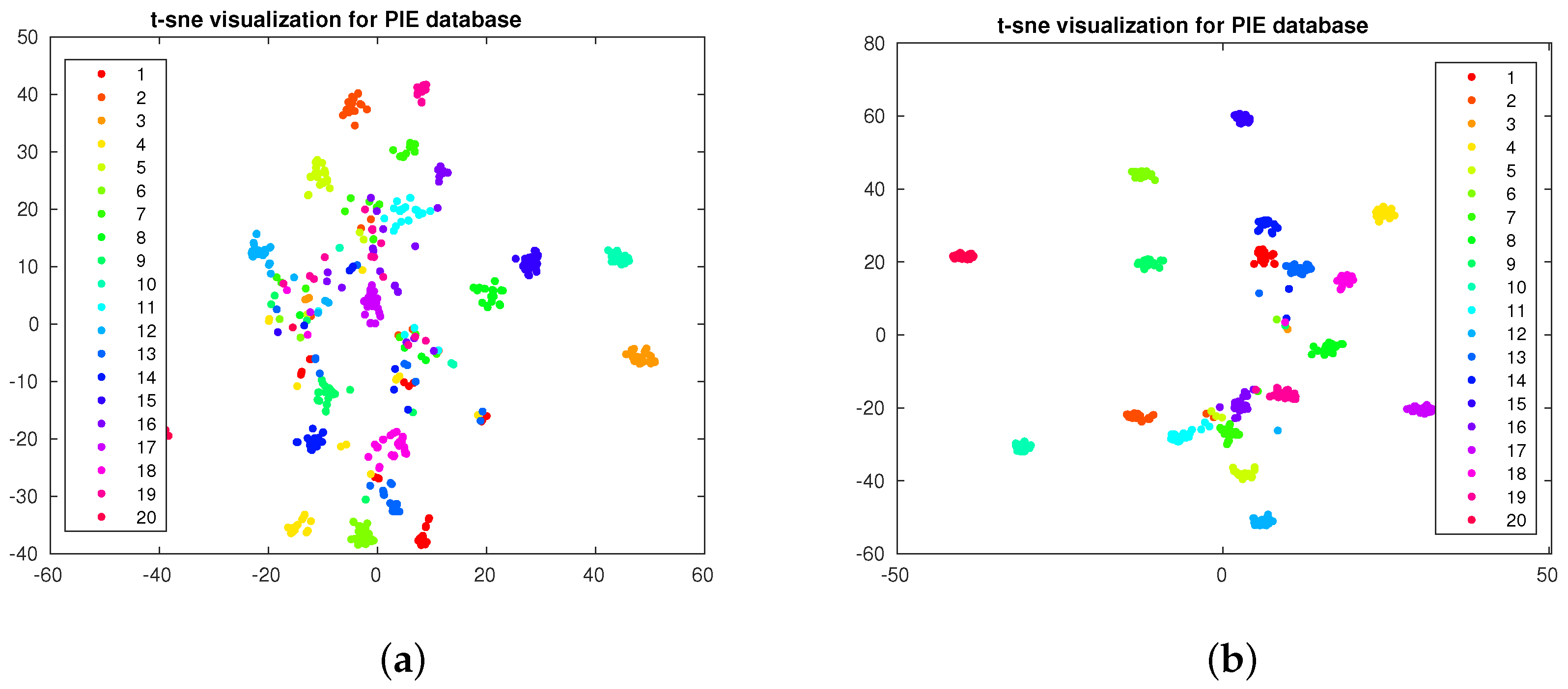
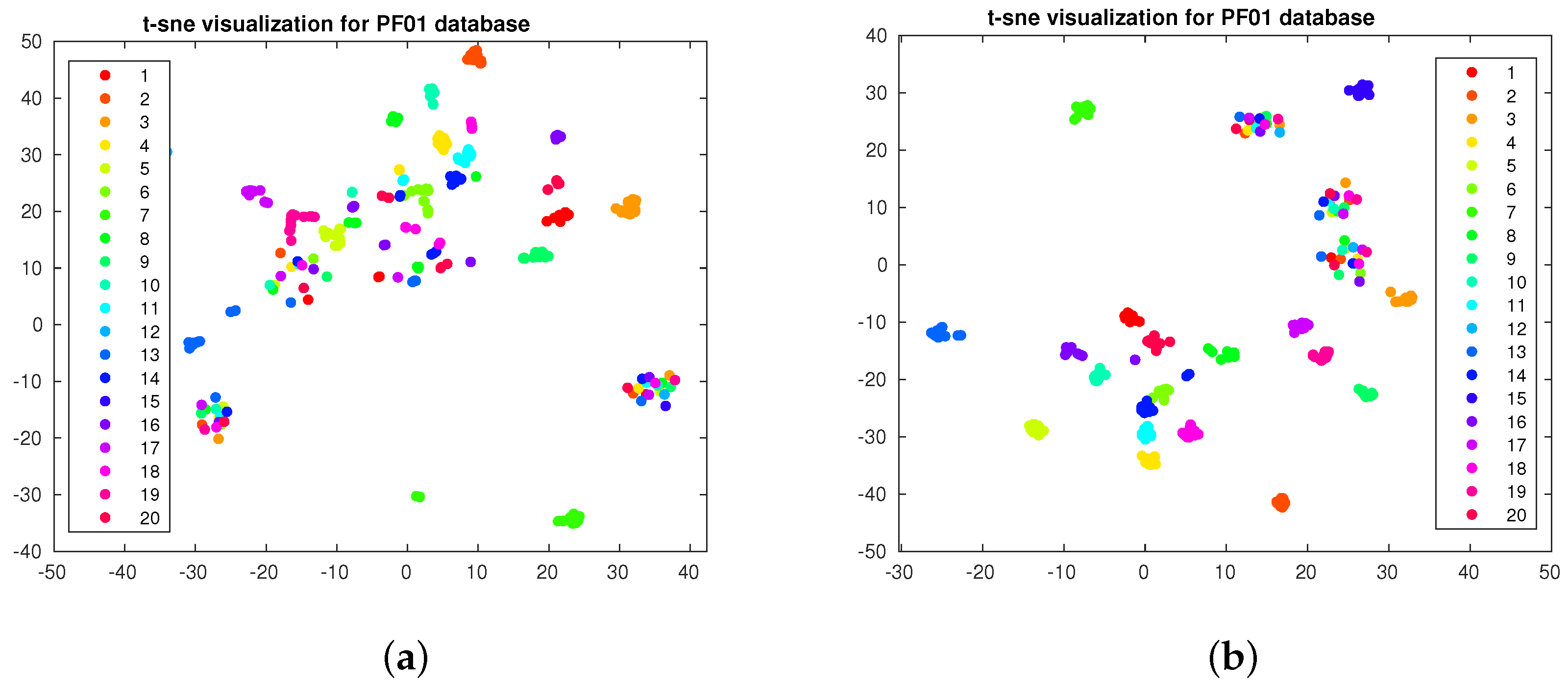
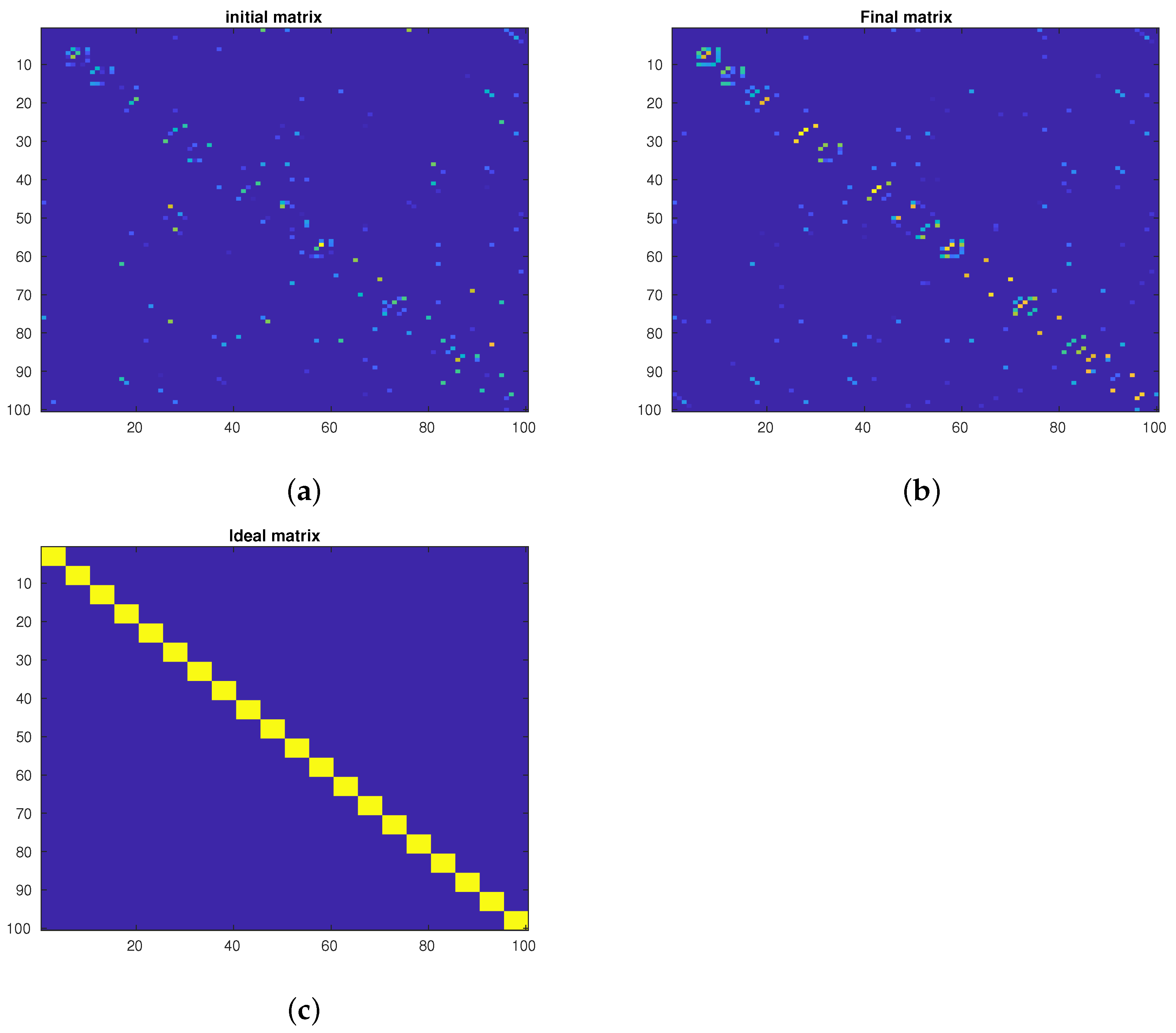
4.3. Data Visualization

In this section, we focus on data visualization to have a visual observation of how the data are distributed after applying the proposed method. It should be noted that, when one proposes an embedding or data transformation algorithm, there exist several ways to evaluate the data projection method. Data visualization methods are qualitative tools that help us to visually observe the calculated embedding. In this article, we proposed an embedding method that receives data features as input and provides several outputs (e.g., labels and affinity matrix). It is common to adopt the label vector of each sample as a sample representation of data in the label space. Apart from numerical comparisons, we use data visualization tools to visually demonstrate the labels of samples along with the consensus affinity matrix as two calculated outputs of the proposed method.
In the first experiment, we want to compare the effect of increasing the number of labeled samples. As the objective of this visualization is comparison, we adopt the scatter plot visualization [40]. We apply the well-known t-SNE [3] algorithm to the PIE and PF01 databases. We apply the t-SNE algorithm on the label matrix calculated by (16) and plot the output for the first 20 classes. In Figure 1a,b, we plot the output for the PIE database when 5 and 15 labels per class are adopted. In Figure 2a,b, we plot the output for the PF01 database when three and five labels per class are adopted. As we observe, the separation between the classes increases when we increase the number of labeled samples. This is what we will also observe in the classification accuracy.
Moreover, as we compare Figure 1a with Figure 1b and Figure 2a with Figure 2b, we observe that increasing the number of labeled samples increases the separability between the classes. However, increasing labeled samples requires human effort and intervention. Moreover, we observe that some classes are completely separated from others—hence, there is no need to increase the number of labeled samples in those classes—while some classes are still mixed and finding a clear class border for them is challenging. Interactive visualization can be useful in this case, as one can visualize the data and the user may only annotate samples of the mixed classes, consequently increasing the separability and enhancing the performance without increasing the number of labeled samples for all classes.
In the second experiment, we focus on the affinity matrix visualization on the PF01 database. Without loss of generality, we rearrange the samples such that the samples in the same class are close to each other. Then, we plot the initial graph (Figure 3a), the final graph (Figure 3b), and the ideal graph (Figure 3c) for the first 100 samples. The initial graph is the one we start the algorithm with. The final graph is the affinity matrix calculated after the last iteration of the proposed method. The ideal graph is our desired graph where we only have edges for the samples in the same class and no link exists between the samples in different classes. For this reason, we artificially create the link only for the within-class samples and no links exist for between-class samples. As we can see, after the optimization process, the final graph (i.e., Figure 3b) is more similar to the ideal graph compared to the initial graph. More precisely, in Figure 3b) we can see points (i.e., edges) between the samples in the same class. It shows that, after the optimization process, the proposed method could find the samples in the same class and create a link between them. In other words, we observe that the links between the samples in the same class are enhanced. As we will see, this phenomenon will be confirmed by the accuracy of the proposed method.

4.4. Small Databases

For the adopted face databases (PIE, PF01, and FERET), which are relatively small, the test set is empty and all samples are adopted for training. From training data, l samples are selected randomly as labeled while the other samples are handled as unlabeled. For small databases that have few samples, we adopt this strategy.
The labels of the unlabeled data are obtained using the estimated matrix, F , the solution of Equation (12). We compute the label estimate over unlabeled samples in 10 combinations of labeled/unlabeled. For the PIE, PF01, and FERET databases, the accuracy for FME with a single descriptor, FME with feature concatenation, and the proposed method is given in Table 2. The highest accuracy between the methods is represented in bold font.
As we can see, the proposed technique can enhance the performance compared to the use of a single descriptor. Moreover, we can see that the fusion performed by the simple feature concatenation in the FME solution can also improve the accuracy compared to the single descriptor. However, compared to single descriptors and concatenation, the proposed algorithm achieves superior performance by showing higher average accuracy and lower standard deviation. It demonstrates that the proposed method can better evoke discriminant data from various descriptors.

4.5. Large Databases

The presence of all samples for training is not the case for real problems. Moreover, for large databases, it is difficult to use all the samples in the training phase, as this requires a lot of memory and increases the computational cost. Therefore, we separate the MNIST database into two parts: train and test. The train set contains both labeled and unlabeled data. It is worth mentioning that the difference between the test samples and the unlabeled samples is that the unlabeled samples are considered as training data; hence, they participate in model estimation, i.e., the underlying manifold. However, test samples are not adopted to train the model.
In the MNIST database, we take 1000 images of each class as train data and leave the rest of the images as unseen or test samples. Similar to small databases, l images in the training set are considered as labeled data and the rest as unlabeled and we compute the accuracy of the correct propagation of labeling of unlabeled and test samples separately. We repeat this setup for 10 combinations of labeled and unlabeled samples, and report the average and standard deviation of the accuracy in Table 3. The highest accuracy between the methods is represented with bold font. We report the accuracy for the unlabeled and test samples separately and compare the proposed method with the following algorithms: SNF [19], SMGI [17], DGFLP [21], MLGC [18], AMGL [31], and MMCL [41].
As we can see for the unlabeled samples, the proposed fusion technique has higher accuracy compared to using a single descriptor, which proves that using data smoothness can increase performance. We also observe that the proposed method is superior to the competing fusion techniques due to two reasons. First, the adopted learning model (simultaneous graph and label estimation) can better estimate the labels. Second, the fusion of the descriptors from different views can also increase the performance of the proposed model.
Moreover, we report the accuracy of the test samples in Table 3. We remark on the fact that for transductive methods (namely, SMGI, DGFLP, MLGC, and AMGL) that cannot work on unseen samples, no accuracy is reported for the test data. Moreover, for the proposed method, we adopt Equation (9) to estimate the label of unseen samples.
Similarly to the results obtained for the unlabeled samples, the results obtained by the proposed method have superior accuracy compared to the use of a single view. Moreover, the close accuracy between the unlabeled samples and the test samples shows that (1) the proposed method can estimate the underlying structure of the data well over the unlabeled samples and (2) the obtained solution does not suffer from over-fitting or under-fitting of the training set.

4.6. Ablation Study

In this section, we perform two ablation studies to evaluate the effect of different parts of the proposed method. We select one set of labeled/unlabeled (i.e., one split) and perform the experiments. From the PF01 database, we select one split with 7 labeled samples per class, and from the PIE database with 17 labeled samples per class.
The first experiment applies the proposed method as explained in the article versus excluding the PCA preprocessing step. As we can see in Table 4, when we exclude the PCA, due to the use of the whole features that can be redundant, noisy, or irrelevant, the accuracy of the proposed method drops (even though this drop is not significant). On the other hand, we can see that we have an increase in the CPU time of the proposed method which is due to the large number of features that lead to larger projection matrices and more unknowns that should be estimated. Hence, the use of PCA, even though it does not significantly increase the accuracy, can significantly reduce the computational time.
In the second ablation study, we evaluate the effect of parameters. According to Equation (12), the main parameters of the proposed method are λ , γ , μ , and α . In each experiment, we set one parameter to zero and keep the rest intact. The results are reported in Table 5. As we observe, the accuracy drops as we eliminate the parameters. However, we can see that the elimination of the term associated with λ has the least effect on the accuracy while the terms weighed by U i i and γ have a crucial contribution to the final classification accuracy.

5. Conclusions

In this paper, we have proposed a semi-supervised learning algorithm that uses the assumption of data smoothness in its minimization framework. Moreover, the proposed method is multi-view, which allows us to utilize the information available in different feature descriptors. In addition, it is a multi-view data visualization method that fuses the information from different sources and encounters a more discriminative yet lower dimension that is more optimal for visualization. Moreover, the proposed unified framework simultaneously estimates the unified graph, the labels of unlabeled samples, and the projection matrix. Since the projection matrix is used to predict the labels of unseen samples, the proposed method is easily applicable to large databases to predict the labels of unseen samples since it does not require the use of the entire data in the training phase. Experimental results show that the proposed method has better performance compared to using a single descriptor and other fusion techniques. Furthermore, via affinity matrix visualization, the current work shows that, inside the iterations, the proposed method allows for more optimal estimations of the relation between the nodes. Also, by adopting the t-SNE visualization, we demonstrate that the estimated embedding in the label space becomes more discriminative as the number of labeled samples increases. It is worth noting that active learning is useful in semi-supervised learning where one can select unlabeled samples to go to human annotation, hence increasing the number of labeled samples. As we observed, using interactive visualization, one can visualize the samples and only select samples close to the class borders for annotation. By doing so, one can increase the separability between the classes without increasing the labeled samples in all classes, consequently reducing the human effort in labeling samples.
One drawback of the proposed method is that it assigns the same weights to different views. However, some descriptors might be more informative compared to others, so adaptively assigning weights to the views can improve the performance.

Author Contributions

Conceptualization, A.B. and F.D.; Data curation, N.Z. and A.B.; Formal analysis, N.Z., A.B., and F.D.; Funding acquisition, A.B. and F.D.; Investigation, N.Z., A.B., and F.D.; Methodology, A.B. and F.D.; Project administration, A.B. and F.D.; Resources, A.B. and F.D.; Software, N.Z. and A.B.; Supervision, A.B. and F.D.; Validation, N.Z. and A.B.; Visualization, N.Z., A.B., and F.D.; Writing—original draft, N.Z., A.B., and F.D.; Writing—review and editing, N.Z., A.B., and F.D. All authors have read and agreed to the published version of the manuscript.

Funding

This research was partially funded by Shahid Rajaee Teacher Training University under grant number 4891 and partially supported by the grant PID2021-126701OB-I00 funded by MCIN/AEI/10.13039/501100011033 and by “ERDF A way of making Europe”.

Data Availability Statement

The data presented in this study are available on request from the corresponding author.

Conflicts of Interest

The authors declare no conflicts of interest. The funders had no role in the design of the study; in the collection, analyses, or interpretation of data; in the writing of the manuscript; or in the decision to publish the results.

References

  1. Li, Q. Overview of Data Visualization. In Embodying Data: Chinese Aesthetics, Interactive Visualization and Gaming Technologies; Springer: Singapore, 2020; pp. 17–47. [Google Scholar] [CrossRef]
  2. Szubert, B.; Cole, J.E.; Monaco, C.; Drozdov, I. Structure-preserving visualisation of high dimensional single-cell datasets. Sci. Rep. 2019, 9, 8914. [Google Scholar] [CrossRef]
  3. van der Maaten, L.; Hinton, G. Visualizing Data using t-SNE. J. Mach. Learn. Res. 2008, 9, 2579–2605. [Google Scholar]
  4. McInnes, L.; Healy, J.; Saul, N.; Großberger, L. UMAP: Uniform Manifold Approximation and Projection. J. Open Source Softw. 2018, 3, 861. [Google Scholar] [CrossRef]
  5. Sainburg, T.; McInnes, L.; Gentner, T.Q. Parametric UMAP Embeddings for Representation and Semisupervised Learning. Neural Comput. 2021, 33, 2881–2907. [Google Scholar] [CrossRef]
  6. Nie, F.; Wang, Z.; Wang, R.; Li, X. Adaptive Local Embedding Learning for Semi-supervised Dimensionality Reduction. IEEE Trans. Knowl. Data Eng. 2021, 34, 4609–4621. [Google Scholar] [CrossRef]
  7. He, F.; Nie, F.; Wang, R.; Hu, H.; Jia, W.; Li, X. Fast Semi-Supervised Learning with Optimal Bipartite Graph. IEEE Trans. Knowl. Data Eng. 2020, 33, 3245–3257. [Google Scholar] [CrossRef]
  8. Dornaika, F.; Bosaghzadeh, A.; Raducanu, B. Efficient Graph Construction for Label Propagation Based Multi-observation Face Recognition. In Human Behavior Understanding; Salah, A.A., Hung, H., Aran, O., Gunes, H., Eds.; Springer: Cham, Switzerland, 2013; pp. 124–135. [Google Scholar]
  9. Bahrami, S.; Bosaghzadeh, A.; Dornaika, F. Multi Similarity Metric Fusion in Graph-Based Semi-Supervised Learning. Computation 2019, 7, 15. [Google Scholar] [CrossRef]
  10. Zheng, F.; Liu, Z.; Chen, Y.; An, J.; Zhang, Y. A Novel Adaptive Multi-View Non-Negative Graph Semi-Supervised ELM. IEEE Access 2020, 8, 116350–116362. [Google Scholar] [CrossRef]
  11. Li, L.; He, H. Bipartite Graph based Multi-view Clustering. IEEE Trans. Knowl. Data Eng. 2020, 34, 3111–3125. [Google Scholar] [CrossRef]
  12. Angelou, M.; Solachidis, V.; Vretos, N.; Daras, P. Graph-based multimodal fusion with metric learning for multimodal classification. Pattern Recognit. 2019, 95, 296–307. [Google Scholar] [CrossRef]
  13. Nie, F.; Tian, L.; Wang, R.; Li, X. Multiview Semi-Supervised Learning Model for Image Classification. IEEE Trans. Knowl. Data Eng. 2019, 32, 2389–2400. [Google Scholar] [CrossRef]
  14. Wang, H.; Yang, Y.; Liu, B.; Fujita, H. A study of graph-based system for multi-view clustering. Knowl.-Based Syst. 2019, 163, 1009–1019. [Google Scholar] [CrossRef]
  15. Manna, S.; Khonglah, J.R.; Mukherjee, A.; Saha, G. Robust kernelized graph-based learning. Pattern Recognit. 2021, 110, 107628. [Google Scholar] [CrossRef]
  16. Kang, Z.; Shi, G.; Huang, S.; Chen, W.; Pu, X.; Zhou, J.T.; Xu, Z. Multi-graph fusion for multi-view spectral clustering. Knowl.-Based Syst. 2020, 189, 105102. [Google Scholar] [CrossRef]
  17. Karasuyama, M.; Mamitsuka, H. Multiple Graph Label Propagation by Sparse Integration. IEEE Trans. Neural Netw. Learn. Syst. 2013, 24, 1999–2012. [Google Scholar] [CrossRef]
  18. An, L.; Chen, X.; Yang, S. Multi-graph feature level fusion for person re-identification. Neurocomputing 2017, 259, 39–45. [Google Scholar] [CrossRef]
  19. Wang, B.; Mezlini, A.M.; Demir, F.; Fiume, M.; Tu, Z.; Brudno, M.; Haibe-Kains, B.; Goldenberg, A. Similarity network fusion for aggregating data types on a genomic scale. Nat. Methods 2014, 11, 333–337. [Google Scholar] [CrossRef]
  20. Bahrami, S.; Dornaika, F.; Bosaghzadeh, A. Joint auto-weighted graph fusion and scalable semi-supervised learning. Inf. Fusion 2021, 66, 213–228. [Google Scholar] [CrossRef]
  21. Lin, G.; Liao, K.; Sun, B.; Chen, Y.; Zhao, F. Dynamic graph fusion label propagation for semi-supervised multi-modality classification. Pattern Recognit. 2017, 68, 14–23. [Google Scholar] [CrossRef]
  22. Nie, F.; Cai, G.; Li, X. Multi-View Clustering and Semi-Supervised Classification with Adaptive Neighbours. In Proceedings of the Thirty-First AAAI Conference on Artificial Intelligence, San Francisco, CA, USA, 4–9 February 2017. [Google Scholar]
  23. Kang, Z.; Peng, C.; Cheng, Q.; Liu, X.; Peng, X.; Xu, Z.; Tian, L. Structured graph learning for clustering and semi-supervised classification. Pattern Recognit. 2021, 110, 107627. [Google Scholar] [CrossRef]
  24. Deng, J.; Yu, J.G. A simple graph-based semi-supervised learning approach for imbalanced classification. Pattern Recognit. 2021, 118, 108026. [Google Scholar] [CrossRef]
  25. Nie, F.; Xu, D.; Tsang, I.W.; Zhang, C. Flexible Manifold Embedding: A Framework for Semi-Supervised and Unsupervised Dimension Reduction. IEEE Trans. Image Process. 2010, 19, 1921–1932. [Google Scholar] [CrossRef]
  26. Zhu, X.; Ghahramani, Z.; Lafferty, J.D. Semi-supervised learning using gaussian fields and harmonic functions. In Proceedings of the 20th International conference on Machine learning (ICML-03), Washington, DC, USA, 21–24 August 2003; pp. 912–919. [Google Scholar]
  27. Zhou, D.; Bousquet, O.; Lal, T.N.; Weston, J.; Schölkopf, B. Learning with Local and Global Consistency. In Advances in Neural Information Processing Systems 16; Thrun, S., Saul, L.K., Schölkopf, B., Eds.; MIT Press: Cambridge, MA, USA, 2004; pp. 321–328. [Google Scholar]
  28. Budd, S.; Robinson, E.C.; Kainz, B. A survey on active learning and human-in-the-loop deep learning for medical image analysis. Med. Image Anal. 2021, 71, 102062. [Google Scholar] [CrossRef]
  29. Tharwat, A.; Schenck, W. A Survey on Active Learning: State-of-the-Art, Practical Challenges and Research Directions. Mathematics 2023, 11, 820. [Google Scholar] [CrossRef]
  30. Ferdinands, G.; Schram, R.; de Bruin, J.; Bagheri, A.; Oberski, D.L.; Tummers, L.; Teijema, J.J.; van de Schoot, R. Performance of active learning models for screening prioritization in systematic reviews: A simulation study into the Average Time to Discover relevant records. Syst. Rev. 2023, 12, 100. [Google Scholar] [CrossRef]
  31. Nie, F.; Li, J.; Li, X. Parameter-free Auto-weighted Multiple Graph Learning: A Framework for Multiview Clustering and Semi-supervised Classification. In Proceedings of the Twenty-Fifth International Joint Conference on Artificial Intelligence IJCAI’16, New York, NY, USA, 9–15 July 2016; AAAI Press: Palo Alto, CA, USA, 2016; pp. 1881–1887. [Google Scholar]
  32. Dong, H.; Gu, N. Asian face image database PF01. 2001. Available online: http://imlab.postech.ac.kr/databases.htm (accessed on 5 January 2006).
  33. Sim, T.; Baker, S.; Bsat, M. The CMU Pose, Illumination, and Expression (PIE) database. In Proceedings of the Fifth IEEE International Conference on Automatic Face Gesture Recognition, Washington, DC, USA, 21 May 2002; pp. 46–51. [Google Scholar] [CrossRef]
  34. Phillips, P.J.; Moon, H.; Rizvi, S.A.; Rauss, P.J. The FERET Evaluation Methodology for Face-Recognition Algorithms. IEEE Trans. Pattern Anal. Mach. Intell. 2000, 22, 1090–1104. [Google Scholar] [CrossRef]
  35. Lecun, Y.; Bottou, L.; Bengio, Y.; Haffner, P. Gradient-based learning applied to document recognition. Proc. IEEE 1998, 86, 2278–2324. [Google Scholar] [CrossRef]
  36. Ahonen, T.; Hadid, A.; Pietikainen, M. Face Description with Local Binary Patterns: Application to Face Recognition. IEEE Trans. Pattern Anal. Mach. Intell. 2006, 28, 2037–2041. [Google Scholar] [CrossRef]
  37. Shen, L.; Bai, L. A review on Gabor wavelets for face recognition. Pattern Anal. Appl. 2006, 9, 273–292. [Google Scholar] [CrossRef]
  38. Tuzel, O.; Porikli, F.; Meer, P. Region Covariance: A Fast Descriptor for Detection and Classification. In Proceedings of the Computer Vision—ECCV 2006, Graz, Austria, 7–13 May 2006; Leonardis, A., Bischof, H., Pinz, A., Eds.; Springer: Berlin/Heidelberg, Germany, 2006; pp. 589–600. [Google Scholar]
  39. Simonyan, K.; Zisserman, A. Very Deep Convolutional Networks for Large-Scale Image Recognition. arXiv 2014, arXiv:1409.1556. [Google Scholar]
  40. Sedrakyan, G.; Mannens, E.; Verbert, K. Guiding the choice of learning dashboard visualizations: Linking dashboard design and data visualization concepts. J. Comput. Lang. 2019, 50, 19–38. [Google Scholar] [CrossRef]
  41. Gong, C.; Tao, D.; Maybank, S.J.; Liu, W.; Kang, G.; Yang, J. Multi-Modal Curriculum Learning for Semi-Supervised Image Classification. IEEE Trans. Image Process. 2016, 25, 3249–3260. [Google Scholar] [CrossRef] [PubMed]
Figure 1. t-SNE visualization for PIE database. (a) Five labeled per class. (b) Fifteen labeled per class.
Information 15 00421 g001
Figure 2. t-SNE visualization for PF01 database. (a) Three labeled per class. (b) Five labeled per class.
Information 15 00421 g002
Figure 3. Visualization of affinity matrices. (a) The initial graph. (b) The final graph. (c) The ideal graph.
Information 15 00421 g003
Table 1. Short description of the adopted databases.
DatasetNum. of ClassesNum. of SamplesNum. of Samples in Each ClassExtracted DescriptorsDimension
PF01107181917Cov [38]405
Gabor [37]2560
LBP [36]900
PIE68192627∼29Cov [38]405
Gabor [37]2560
LBP [36]900
FERET20014007Cov [38]405
Gabor [37]2560
LBP [36]900
MNIST1060,0005421∼6742VGG16 [39]4096
VGG19 [39]4096
Table 2. Results obtained by the proposed method and FME with a single descriptor. Concatenation of the features is also treated as a single descriptor. The table shows the average and standard deviation of accuracy obtained on ten splits.
PIE
MethodCovGaborLBPConcat.JGC-MFME
Num. of Lab. Samples/Class
1580.93 ± 3.7191.79 ± 3.3287.75 ± 3.9094.31 ± 2.8894.44 ± 2.76
1781.93 ± 4.0691.09 ± 3.0888.11 ± 2.9994.54 ± 2.5194.75 ± 2.58
FERET
MethodCovGaborLBPConcat.JGC-MFME
Num. of Lab. Samples/Class
359.17 ± 9.5379.80 ± 8.9672.01 ± 10.383.98 ± 8.0685.50 ± 7.64
567.27 ± 18.6786.00 ± 15.3885.15 ± 17.6690.72 ± 12.9891.77 ± 12.98
PF01
MethodCovGaborLBPConcat.JGC-MFME
Num. of Lab. Samples/Class
570.24 ± 3.3484.26 ± 3.7679.57 ± 2.5591.30 ± 2.0392.28 ± 1.61
771.82 ± 5.9385.81 ± 4.9380.71 ± 4.5193.22 ± 2.3994.13 ± 2.01
Table 3. Results on MNIST database for different labeled and unlabeled combinations and three different numbers of labeled samples. (Top) Over the unlabeled samples which are estimated by the algorithms. (Bottom) Over the test samples estimated via the linear projection of FME algorithm.
MNIST (Accuracy on Unlabeled Data)
Lab./class203040
Method
Single descriptor (VGG16)94.53 ± 0.395.17 ± 0.395.59 ± 0.3
Single descriptor (VGG19)94.35 ± 0.594.99 ± 0.595.35 ± 0.4
Feature Concat.95.87 ± 0.496.28 ± 0.496.66 ± 0.3
SNF [19]94.53 ± 0.695.81 ± 0.496.49 ± 0.3
SMGI [17]88.40 ± 0.989.66 ± 0.789.84 ± 0.7
DGFLP [21]92.14 ± 0.592.70 ± 0.593.06 ± 0.3
MLGC [18]88.20 ± 1.489.45 ± 1.090.27 ± 0.7
AMGL [31]94.99 ± 0.595.39 ± 0.395.67 ± 0.3
MMCL [41]52.45 ± 14.549.98 ± 13.949.22 ± 13
JGC-MFME95.91 ± 0.496.34 ± 0.496.68 ± 0.3
MNIST (Accuracy on Test Data)
Lab./class203040
Method
Single descriptor (VGG16)94.98 ± 0.595.39 ± 0.395.81 ± 0.3
Single descriptor (VGG19)95.05 ± 0.595.64 ± 0.495.97 ± 0.4
Feature Concat.95.47 ± 0.596.79 ± 0.596.21 ± 0.4
SNF [19]94.79 ± 0.695.97 ± 0.396.64 ± 0.2
JGC-MFME95.92 ± 0.495.36 ± 0.396.76 ± 0.3
Table 4. The effect of using PCA on the performance of the proposed method.
DatabaseEvaluation MetricProp. MethodProp. Method (Without PCA)
PF01 7 labeledAcc (%)95.1493.36
CPU time (Sec)2365
PIE 17 labeledAcc (%)90.1289.61
CPU time (Sec)2047
Table 5. Parameter ablation study. In this experiment, we evaluate the effect of each parameter by setting it to zero.
DatabaseProp. Method λ = 0 α = 0 μ = 0 U ii = 0 γ = 0
PF01 7 labeled95.1494.9560.8460.840.930.93
PIE 17 labeled90.129066.166.11.551.55
Disclaimer/Publisher’s Note: The statements, opinions and data contained in all publications are solely those of the individual author(s) and contributor(s) and not of MDPI and/or the editor(s). MDPI and/or the editor(s) disclaim responsibility for any injury to people or property resulting from any ideas, methods, instructions or products referred to in the content.

