Utilizing Multi-Class Classification Methods for Automated Sleep Disorder Prediction

Abstract

Even from infancy, a human’s day-life alternates from a period of wakefulness to a period of sleep at night, during the 24-hour cycle. Sleep is a normal process necessary for human physical and mental health. A lack of sleep makes it difficult to control emotions and behaviour, reduces productivity at work, and can even increase stress or depression. In addition, poor sleep affects health; when sleep is insufficient, the chances of developing serious diseases greatly increase. Researchers in sleep medicine have identified an extensive list of sleep disorders, and thus leveraged Artificial Intelligence (AI) to automate their analysis and gain a deeper understanding of sleep patterns and related disorders. In this research, we seek a Machine Learning (ML) solution that will allow for efficient classification of unlabeled instances as being Sleep Apnea, Insomnia or Normal (subjects without a specific sleep disorder) by assessing the performance of two well-established strategies for multi-class classification tasks: the One-Vs-All (OVA) and One-Vs-One (OVO). In the context of the specific strategies, two well-known binary classification models were assumed, Logistic Regression (LR) and Support Vector Machines (SVMs). Both strategies’ validity was verified upon a dataset of diverse information related to the profiles (anthropometric data, sleep metrics, lifestyle and cardiovascular health factors) of potential patients or individuals not exhibiting any specific sleep disorder. Performance evaluation was carried out by comparing the weighted average results in all involved classes that represent these two specific sleep disorders and no-disorder occurrence; accuracy, kappa score, precision, recall, f-measure, and Area Under the ROC curve (AUC) were recorded and compared to identify an effective and robust model and strategy, both class-wise and on average. The experimental evaluation unveiled that after feature selection, 2-degree polynomial SVM under both strategies was the least complex and most efficient, recording an accuracy of 91.44%, a kappa score of 84.97%, precision, recall and f-measure equal to 0.914, and an AUC of 0.927.

1. Introduction

In scientific terms, sleep is a state of different consciousness and limited interaction with the environment, during which the body’s sensory functions and voluntary muscle movements are suspended. The exact processes that take place in the brain and the rest of the body during sleep are complex and still under investigation. Sleep is necessary and refreshing since it fills us with energy and helps us cope with the demands of everyday life. When the body is deprived of good sleep, its health balance is disturbed [1]. The World Sleep Society, in its effort to raise the awareness of both the public and health professionals about the importance of a sufficient quantity and quality of sleep, has established World Sleep Day on the last Friday before the Vernal Equinox each year [2].

Sleep alternates between two different types: REM (rapid eye movement) sleep and non-REM sleep. It starts with non-REM sleep, which is made up of four different stages. The first stage is an intermediate state between wakefulness and sleep. The second stage involves light sleep, during which the heart rate slows, breathing slows, and body temperature drops. In the third and fourth stages, we have deep sleep. Then we enter REM sleep, which is characterized by rapid eye movements with the eyelids closed. During this phase, brain waves resemble those we have when we are awake. The rate of breathing increases, and our muscles become temporarily paralyzed as we dream [3,4].

Adequate sleep is when one wakes up feeling refreshed without feeling sleepy or tired during the day. The amount of sleep that is necessary varies from person to person and is affected by various factors such as age, heredity, daily activities, lifestyle, exercise, etc. [5,6]. Protecting sleep is important in infancy and childhood because it has an important role in development. Newborn children sleep 16–18 h, but at the age of 3, the average sleep duration is 11–13 h. Sleep after 4 years of age is a stable and continuous nocturnal period of 10 h until 12–13 years of age when pre-adolescence and the endocrinological changes associated with it begin. Sleep duration after puberty ranges from 7–9 h and gradually decreases as a person ages [7,8].

Sleep contributes to the proper functioning of the brain and body as they undergo restoration and repair. Good sleep helps the hormones function properly and therefore maintain weight. The hormones that affect sleep are ghrelin (a hormone that increases the feeling of hunger) and leptin (a hormone that regulates the feeling of satiety from eating). When sleep is not sufficient, the balance of these hormones is disturbed, resulting in an increased feeling of hunger. Sleep lowers stress levels; therefore, blood pressure is better controlled [9,10]. Moreover, sleep is important during childhood and adolescence because growth hormone is secreted during deep sleep [11,12]. When the duration or quality of sleep is reduced, there is a greater risk of arterial hypertension, cardiovascular diseases, diabetes, and obesity as the metabolism is affected and the immune system is generally weakened. In addition, in some cases, there is a decline in cognitive functions, e.g., memory and concentration, as well as fatigue that reduces performance at work. Extensive sleep loss also leads to depression [13,14,15]. Many adults face sleep problems related either to its quality or to its quantity [16].

An international classification of sleep disorders [17] discriminates them into insomnia, sleep-related breathing (e.g., sleep apnea disorders), sleep-related movement disorders, parasomnia (e.g., (N)REM-related sleepwalking), central disorders of hypersomnolence (e.g., narcolepsy), circadian rhythm sleep-wake disorders, etc. According to [18], sleep disorders that affect a wide number of people span into insomnia, sleep apnea, periodic limb movement, REM sleep behaviour and bruxism; sleep apnea and insomnia are the two most prevalent and investigated disorders while narcolepsy and nocturnal frontal lobe epilepsy are less common sleep disorders with low prevalence.

Among primary caregivers, medical practitioners and physicians, two key screening methods have been identified for measuring sleep parameters: (i) objective measures based on physiological signals acquired through Polysomnography-PSG (PSG can be used to capture brain electrical activity, muscle activity, eye movements, respiratory rate and other channels) in either a laboratory or a home environment) [19], and (ii) subjective, self-reported questionnaires [20,21]. In ref. [22], the authors introduced a combined method that is based on the most commonly used tool, the Pittsburgh Sleep Quality Inventory (PSQI), and an objective sleep quality scoring system that gathers daily sleep data from a smart device (specifically, a smartwatch). This method emphasized triggering mechanisms based on behavioural and lifestyle routines to assist an automated system in correcting the results for personalized scoring for each user. Also, ref. [23] aimed to combine the applied sleep quality measurement methods of previous research on rich information data and explore the possibility of advice when sleep health deteriorates. Although objective methods are highly reliable in obtaining sleep-related parameters, they are expensive, time-consuming and thus prohibitive. On the other hand, subjective methods are low-cost, easy to use, reduce interventions from medical experts and are advantageous, providing compliance, consistency and validity.

The leverage of AI and ML has gained considerable attention for automating and adding intelligence in various fields of the healthcare sector and specifically towards medical science providing clinicians with valuable tools for monitoring, tracking early signs/symptoms, risk assessment, and predicting various diseases, such as cardiovascular diseases [24], chronic obstructive pulmonary disease [25], SARS-CoV-2 [26], hypertension [27], metabolic syndrome [28], breast cancer [29], stroke [30], cholesterol [31] etc. AI in sleep medicine for automating the identification of sleep disorders has also attracted researchers’ and medical experts’ interest [32]. Several types of devices have helped them collect data suitable for representing sleep statuses which, in conjunction with self-rated questionnaires, will play an essential role in diagnosing several sleep disorders.

The use of wearable devices equipped with sensors can continuously monitor physiological signals such as heart rate, oxygen saturation, and respiratory patterns [33]. These devices, often integrated with smartphones or other mobile devices, collect real-time data that can be analysed using sophisticated algorithms to detect anomalies indicative of, e.g., sleep apnea events. For instance, a sudden drop in oxygen levels or irregular breathing patterns can be identified and flagged. The integration of ML models, particularly deep learning (DL) techniques, enhances the accuracy of detection by learning from large datasets of labelled sleep patterns, thereby improving the system’s ability to recognize subtle indicators of sleep apnea. DL models (e.g., Convolutional Networks) can be used to simultaneously detect sleep stages, besides the sleep disorder from multimodal sensors, which is known as multi-task classification [34]. The problem with the simultaneous prediction of multiple outcomes (stage, disorder) is not new but it has been applied to other diseases previously using revised stacking algorithms [35].

In this article, following a supervised learning procedure, our primary goal is to formulate a single-task multi-class classification framework that discerns a certain sleep disorder among multiple ones through specific feature-signs observation. To achieve this, we developed high-sensitivity and accuracy ML models that classify unknown subjects to the disorder they are truly suffering from. The main aspects of the adopted methodology are the following:

• Firstly, raw data analysis is applied to understand nominal features’ frequency of occurrence and the most representative category and identify their relatedness with the sleep disorder classes. Also, a statistical analysis of numerical features is presented in the whole dataset and per class group. One-way analysis of variance (ANOVA) [36] was applied to identify if there are differences in means among the three groups’ numerical features. Due to the rejection of means equality (null hypothesis), we proceeded to the Tukey–Kramer post hoc test to find which pairs were different.
• Secondly, emphasis is given to the feature-wise pre-processing step to ensure that feature data are correctly captured before feeding them to the block which is responsible for the prediction models’ training. For this purpose, an unsupervised filter is applied to turn attributes with discrete/categorical numeric values into nominal ones. Also, numerical data normalization is applied.
• Thirdly, pre-processing is followed by feature analysis to measure their importance to the sleep disorder class variable by selecting random forests (RFs) and, specifically, the Gini impurity index and information gain (InfoGain) methods.
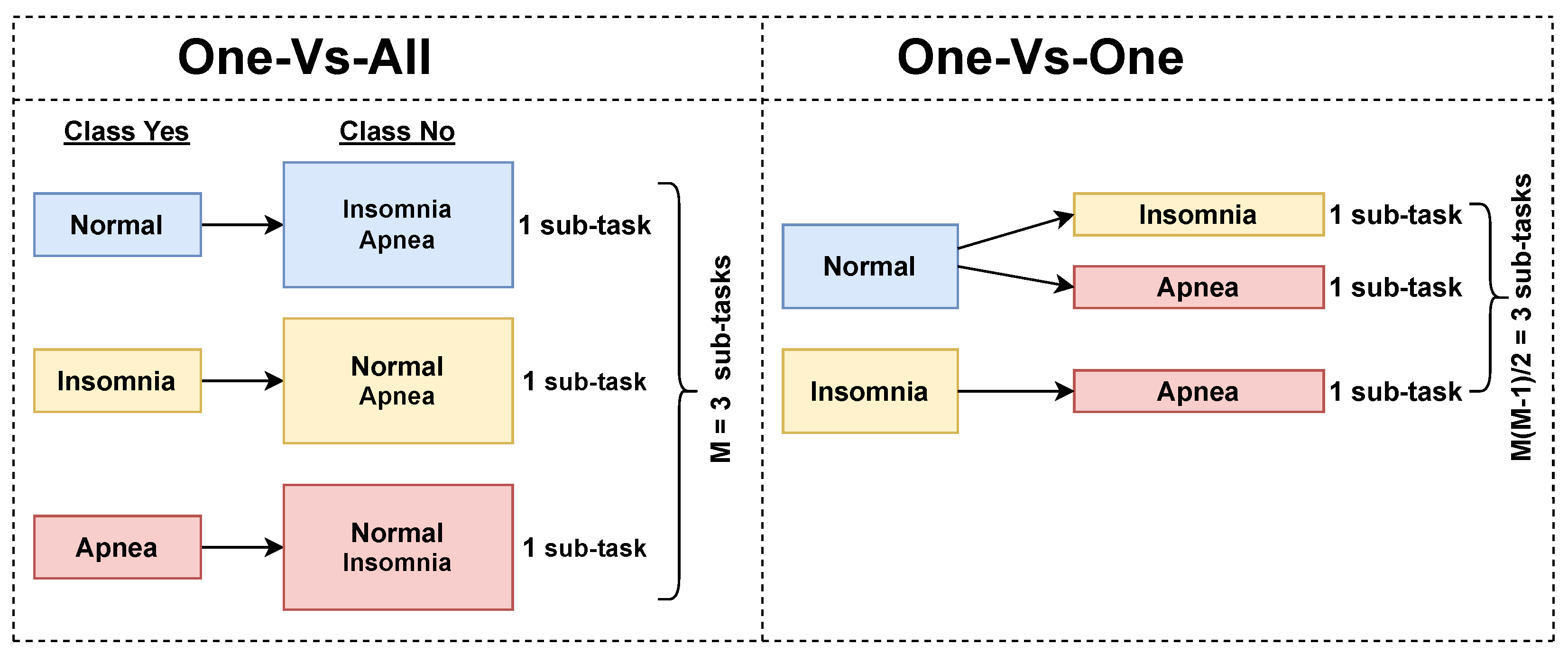
• Finally, a sleep disorder prediction approach is analytically presented where two well-known decomposition strategies, OVA and OVO, are adapted to the problem under consideration and are evaluated assuming LR and SVM as base models for building the 2-class classifiers involved in the internal mechanism of each strategy. To decide which of these strategies is more efficient, we considered two experimental cases, one with all available features and one after feature selection, where accuracy, kappa score (K), precision, recall, f-measure, and AUC metrics were measured and compared. All metrics unveiled that, irrespective of the strategy, 2-degree polynomial SVM prevailed over the other combinations; thus, it is the main proposition of this analysis.

This research article is organized as follows. In Section 2, we outline related works for the subject under consideration. Moreover, in Section 3, we describe the dataset we relied to and analyse the adopted methodology. Next, in Section 4, we note the experimental results of the ML models and illustrate their performance. Finally, in Section 5, we summarize our research outcomes and discuss possible future directions.

2. Related Works

This section focuses on related works that exploited ML techniques and models as a benchmark for the automated detection of a sleep disorder. The studies about obstructive sleep apnea (OSA) dominate amongst the studies of the rest of the sleep disorders considering the apnea–hypopnea index (AHI) scoring as an additional diagnostic measure that helps to determine the severity level. Then, these data are utilized for training efficient models either solving a binary (e.g., OSA and Non-OSA) or multi-class classification problem (e.g., normal, mild, moderate, and severe OSA).

Firstly, ref. [37] aimed to identify acoustic biomarkers indicative of the severity of sleep-disordered breathing (SDB) by analyzing the breathing sounds collected during an entire overnight sleep. The authors classified the subjects into four SDB severity groups according to the AHI. In this approach, the simple Logistic model achieved an accuracy of 88.3%. Also, the authors approached the problem as a binary classification, dividing the patients into two groups according to whether the patient’s AHI value is lower than a certain threshold; the simple Logistic model reached an accuracy of 92.5%.

Moreover, ref. [38] used a dataset (demographic characteristics, spirometry values, gas exchange, symptoms, etc.) of 313 patients with OSA syndrome and applied two distinct approaches: (1) training regression models (Mean Learner, Linear Regression (LR), k-nearest neighbour (k-NN), Regression Tree (RT), Support Vector Regression (SVR), AdaBoost-SVR) to predict the values of feature AHI, apply thresholding and, thus, identifying the severity level of OSA; and (2) training classification models (Majority Vote, Naive Bayes (NB), k-NN, Classification Tree (CT), Random Forests (RFs), SVM, AdaBoost-SVM) to predict the severity class of potential OSA patients. The authors applied SMOTE (synthetic minority oversampling technique) to balance the dataset and several feature ranking/selection techniques to select the minimum number of features that yield the best performance values. After SMOTE with 10-fold cross-validation, the results showed the superiority of SVM and RF for severity class prediction.

The authors in ref. [39] used a dataset which comprises 1042 subjects diagnosed with OSA characterized by four severity levels (normal, mild, moderate, severe). They used simple clinical measures and regression models to predict the continuous value of the AHI that measures the apnea events per hour. Then, based on the value of this index and relevant thresholding rules, they decided on the severity level. Several models’ (28 for the regression task and 32 for the classification task) performance were evaluated by comparing the original unbalanced data with the class-balanced data (obtained after oversampling) and selection was attributed to reducing the complexity of the problem. The results showed that the extremely randomized trees performed better on all metrics for both tasks (regression and classification).

Sleep stage classification plays a vital role in assessing sleep quality and several works target it. In ref. [40], an unobtrusive system (without wearable devices) was designed and tested consisting of a sleep stages detection module and a sleep position classification module for long-term sleep monitoring. The system exploits a sensing technique based on pressure sensors that detect patients’ movements and bed posture. Several supervised learning algorithms (NB, LR, k-NN, HyperPipes, Decision Tables and RF) were used to accurately infer sleep duration and user positions. Assuming and combing the 2 h data of three users, the RF was the most efficient, reaching an accuracy of ∼95%. Additionally, in ref. [41], an efficient technique for sleep stage classification based on EEG signal analysis using ML algorithms is proposed. EEG signals were filtered and decomposed into frequency sub-bands using a band-pass filter. The RF model dominated against the other models, achieving an accuracy of 97.8%. In the study [42], ML models were applied for sleep apnea detection with unattended sleep and monitoring at home. The authors provided different combinations with 27 classifiers and 4 sleep signals. The Convolutional Neural Network (CNN) achieved accuracy up to 89.41% (kappa 0.7877) when simultaneously using all four signal types (nasal airflow (N), oxygen saturation (O), respiratory effort from the chest (C), and abdomen (A)) monitored with the Nox-T3 device and up to 85.43% (kappa 0.7080) accuracy with only one.

Furthermore, in ref. [43], the authors aimed to automate sleep stage classification by experimenting with several traditional ML algorithms (k-NN, SVM, RF, Decision Tree (DT), NB, Gaussian NB, Multinomial NB, Linear and Quadratic Discriminant Analysis) and, neural networks (multilayer perceptron (MLP), Long Short-Term Memory networks (LSTMs)) using the same data and feature set. For this purpose, they exploited two EEG signals at Fpz-Cz and Pz-Cz electrode locations, one Electrooculography signal (EoC) with a horizontal placement, one EoC signal at the submental area, and one oronasal respiration signal. An extensive analysis of all methodological steps was presented, emphasizing EEG signal pre-processing, feature extraction and selection and carrying out a comparative study with classifiers as mentioned above. SVM under radial basis kernel function and RF were ranked among the best classical models.

A recent work [44] reviewed 95 articles focusing on the physiological signals (ECG, PSG, EEG) and the ML/DL algorithms used for some sleep disorders’ detection, such as sleep apnea, insomnia, REM behaviour, hypopnea, narcolepsy, periodic limb movement disorder, nocturnal frontal lobe epilepsy and bruxism detection. In sleep apnea—the most prevalent disorder—SVM was the most popular ML method followed by an Extreme Learning Machine (ELM). Few studies used approaches that combine ML and DL algorithms. Furthermore, from the DL-based studies, the CNN was the most used algorithm, followed by Long Short-Term Memory (LSTM). Insomnia was the second most often studied sleep disorder where the authors mainly employed SVM and RF (namely, ML methods) while two works focused on CNNs (DL methods). Concerning hypopnea, only DL models were used, an RNN and CNN. For the rest of the abovementioned sleep disorders, the specific review paper presented very few works that selected only ML methods.

The study [45] combined various ML models to predict OSA severity, including gradient boosting models (XGBoost, LightGBM, CatBoost) and Random Forest [46]. Clustering algorithms such as hierarchical agglomerative clustering, K-means, and the Gaussian mixture model were also utilized. Performance metrics showed high classification accuracies: 87.52% (CatBoost for mild OSA), 86.01% (LightGBM for moderate OSA), and 91.11% (LightGBM for severe OSA). Feature engineering techniques further improved model performance, highlighting the potential of ML in predicting OSA severity without performing PSG.

In the study by ref. [47], an intelligent system was presented to prevent and diagnose potential patients with sleep apnea symptomsn early. The system can determine different alerts for sleep apnea associated with different AHI levels. A series of ML algorithms were deployed and worked with a corrective block based on an Adaptive Neuro-Based Fuzzy Inference System and a heuristic algorithm. The initial results from the performance evaluation of the proposed decision support system achieved AUC values in the range of 0.8–0.9 and Matthews correlation coefficient values close to 0.6 with the contribution of several ML models and techniques. Also, in a recent study [48], the same authors presented a promising OSA risk assessment tool using heterogeneous inferential approaches that were based not only on objective data related to the patient’s health profile derived from electronic health records (as previous studies considered) but also on subjective data related to the OSA symptoms reported by the patient. As a result, two risk indicators were considered; a statistical one to determine the severity of the patient’s condition (by thresholding the AHI index to identify OSA and non-OSA classes) and a symbolic one based on OSA symptoms using the fuzzy logic and the concept of membership (not the probability). The proposed intelligent system was exemplified in a case study as a proof of concept, which provided an introduction to the tool, demonstrating its encouraging results.

Comparing our proposition to previous studies, we adopted a multi-class classification approach to categorise an unseen subject as Sleep Apnea, Insomnia or Normal (none of them). For this purpose, the traditional ML pipeline was followed, assuming two well-established methods, OVA and OVO, and using SVM and LR as the base models of these techniques (training and testing) to solve the inherent 2-class classification sub-problems. Unlike our research study, previous studies apply multi-class classification on OSA condition severity level. Differently from the above studies that emphasized objective data acquired from physiological signals, we exploited a mixture of objective and subjective data obtained via questionnaires, describing the daily habits, sleep metrics (duration, quality), lifestyle factors and cardiovascular health of involved subjects. Finally, it should be noted that after feature selection, polynomial SVM was the most efficient model under both strategies, recording promising results in terms of accuracy, K, precision, recall, f-measure and AUC.

3. Materials and Methods

The purpose of this section is manifold. Firstly, it provides a detailed description and analysis of the dataset that will be used for the evaluation of the proposed approach. Secondly, it emphasizes data pre-processing and two methods for measuring the features’ importance which will be utilized in the experiments for feature selection. Thirdly, it presents two multi-class classification strategies, OVA and OVO and how they are formulated for classifying a subject into one of the three classes that capture sleep disorders. Moreover, it describes the ML models that were selected for solving the 2-class classification tasks in each strategy. Moreover, it presents an analysis of the confusion matrix and a definition of the related performance metrics (accuracy, kappa score, precision, recall, f-measure and AUC) for the concept of multi-class classification.

3.1. Dataset Description

The data was based on the National Health and Nutrition Examination Survey and the reports obtained via questionnaires covering several factors indicating sleep patterns related to daily habits, sleep metrics (duration, quality), lifestyle factors and cardiovascular health. More specifically, the dataset comprises 374 records and 14 variables. The key features of the dataset include the following:

• Age (years): The age of the person in years.
• Gender: The person’s gender (Male/Female).
• Occupation: The occupation or profession of the person.
• Sleep Duration (hours): The number of hours the person sleeps per day.
• Quality of Sleep—QoSleep (scale: 1–10): A subjective rating of the quality of the person’s sleep, ranging from 1 to 10.
• Physical Activity Level (minutes/day): The number of minutes the person engages in physical activity daily.
• Stress Level (scale: 1–10): A subjective rating of the stress level experienced by the person, ranging from 1 to 10.
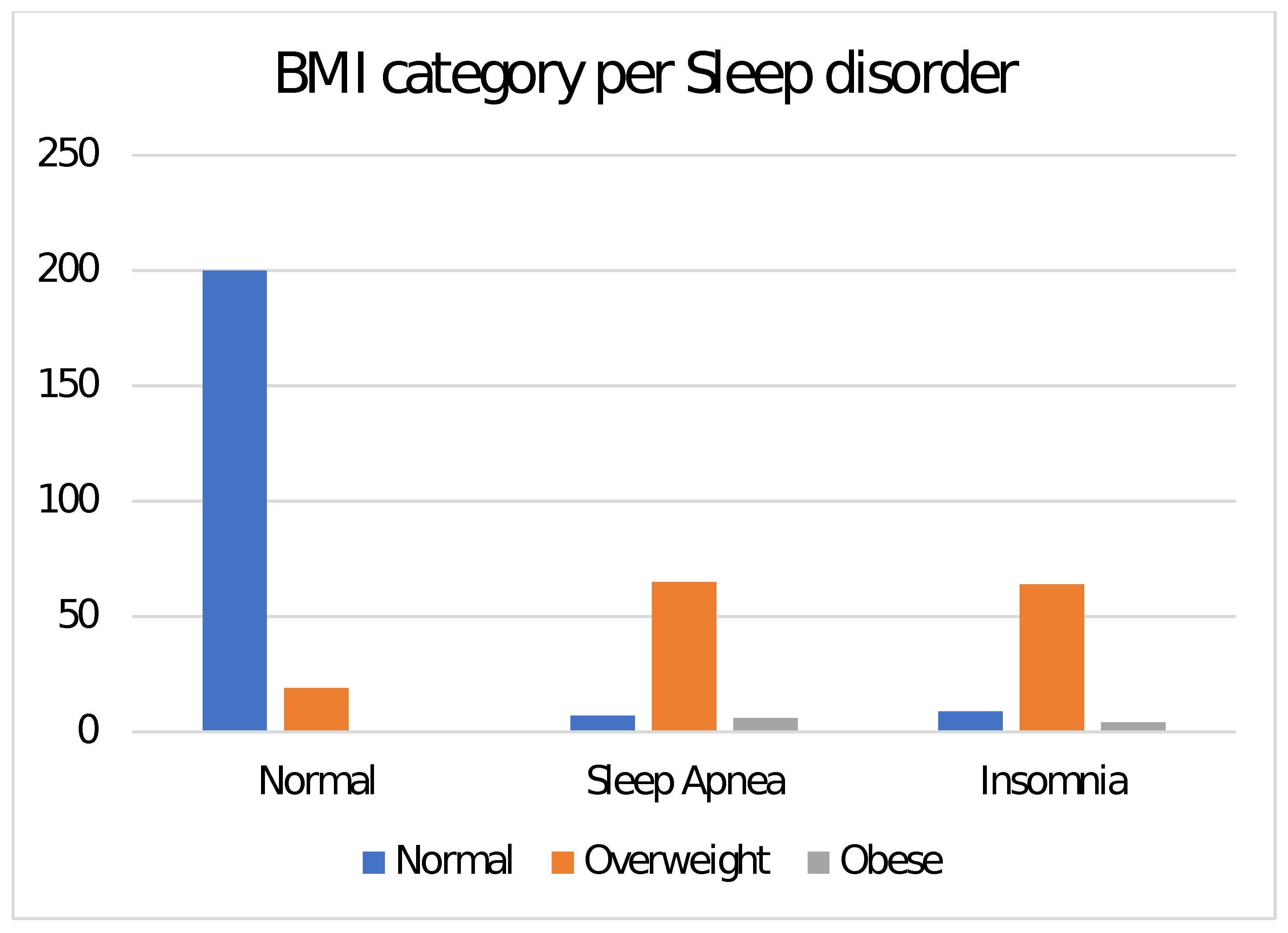
• Boby Mass Index (BMI) Category: The BMI category of the person (e.g., Underweight, Normal, Overweight).
• Blood Pressure (mmHg): The blood pressure measurements for the person, indicated as systolic blood pressure (SysBP) over diastolic blood pressure (DiasBP).
• Heart Rate (bpm): The resting heart rate of the person in beats per minute.
• Daily Steps: The number of steps the person takes daily.
• Asthma: A nominal feature that captures if a subject suffers from asthma or not.
• Sleep Disorder: This feature relates to the class variable and, thus, captures the presence or absence of a sleep disorder in the person spanning into Normal (219 instances), Sleep Apnea (78 instances) and Insomnia (77 instances) categories.
  • Normal: The individual does not exhibit any specific sleep disorder.
  • Insomnia: The individual experiences difficulty falling or staying asleep, leading to inadequate or poor-quality sleep.
  • Sleep Apnea: The individual suffers from pauses in breathing during sleep, resulting in disrupted sleep patterns and potential health risks.

Also, the dataset includes two types of features, numeric and categorical. Sleep quality and stress level are two categorical and specifically ordinal features with intrinsic ordering to their categories on a scale of 1 to 10. Other categorical features with no specific ordering on their categories, thus called nominal, are gender, BMI category, occupation, asthma and having a sleep disorder. The characteristics of the whole dataset are demonstrated in

Table 1. Statistical description of the numerical attributes in the whole dataset.

	Mean ± Stdv	Min–Max
Age	42.18 ± 8.67	27–59
SysBP	128.58 ± 7.75	115–142
DiasBP	84.14 ± 5.66	75–95
HeartRate	71.71 ± 6.25	65–95
Steps	4224.59 ± 2905.87	500–10,000
Sleep Duration	7.13 ± 0.77	5.8–8.5
Physical Activity	39.73 ± 30.30	0–90

presenting their statistical information (the minimum, maximum, mean and standard deviation of their values).

3.2. Dataset Analysis

Isolating the left columns of each sleep disorder in

Table 2. ANOVA of numerical attributes according to the sleep disorder (class label).

	Normal		Sleep Apnea		Insomnia
	Mean	Variance	Mean	Variance	Mean	Variance	p-Value
Age	39.04	61.27	43.52	23.12	49.71	80.83	8.85 $\times {10}^{-23}$
SysBP	124.05	32.29	137.77	26.44	132.17	14.93	4.45 $\times {10}^{-63}$
DiasBP	80.91	14.27	90.54	24.75	86.86	11.41	1.08 $\times {10}^{-57}$
HeartRate	69.29	11.32	78.92	48.59	71.27	39.59	1.21 $\times {10}^{-37}$
Daily Steps	5550.23	7,488,291.23	2378.21	4,832,375.96	2324.68	2,847,146.28	0
Sleep Duration	7.36	0.536	7.03	0.950	6.59	0.149	7.16 $\times {10}^{-29}$
Physical Activity	50.59	927.86	26.15	534.36	22.59	477.37	4.75 $\times {10}^{-17}$

, at first sight, there were differences in the three groups on the basis of age, blood pressure, daily steps, heart rate and physical activity. The mean age of the healthy group was 39 years old, while the mean age of subjects suffering from “Sleep Apnea” and “Insomnia” was 43 and 49 years old. Insomnia seems to mainly concern older adults (subjects around 50 years old) whose mean age was higher than the mean age of the healthy adults [49].

Systolic and diastolic blood pressure and heart rate noted the highest mean values in the “Sleep Apnea” class. The highest mean of sleep duration was reported by subjects belonging to the “Normal” class while there were no important differences among the three groups. Moreover, patients with “Sleep Apnea” presented with higher mean diastolic and systolic blood pressure than “Normal” subjects or those suffering from “Insomnia”. Also, patients with “Sleep Apnea” and “Insomnia” presented with lower average sleep durations, physical activity and daily steps than “Normal” subjects. “Normal” subjects were more physically active than patients, with an average duration of 50.6 min and an average number of steps of around 5550, which is at least twice the time and steps dedicated by “Sleep Apnea” and “Insomnia” subjects.

To statistically validate the significance of the feature means among the groups, the one-way ANOVA was applied; it is a statistical test to check whether there is a difference in means of one variable across multiple groups. Here, we compare the means of the three sleep disorder groups assuming one feature variable per time. Following the one-way ANOVA, the null hypothesis ($H_0$) and the alternative hypothesis ($H_1$), for (numerical) feature i are as follows:

• $H_0:{\mu }_{i1}={\mu }_{i2}={\mu }_{i3}$.
• $H_1:{\mu }_{i1}\ne {\mu }_{i2}$ or ${\mu }_{i1}\ne {\mu }_{i3}$ or ${\mu }_{i2}\ne {\mu }_{i3}$.

In Table 2, we demonstrate the outcomes of the one-way ANOVA (stratified by sleep disorder). The p-value of the features was quite a bit smaller than the statistical significance level $\alpha =0.05$, indicating that there seems to be a difference in means across the three groups, rejecting the null hypothesis $H_0$. Therefore, we further conducted the Tukey–Kramer post hoc test to explore the difference between the group means and the statistical significance per pair of groups.

To determine which group means were different, we compared the absolute mean difference between each pair to the ${\mathrm{Q}}_{\mathrm{critical}}$ value. If the absolute difference in means, noted as AbsDiff, is larger than the ${\mathrm{Q}}_{\mathrm{critical}}$ value, the difference between the groups’ means is statistically significant, where ${\mathrm{Q}}_{\mathrm{critical}}=\mathrm{q}\sqrt{{\displaystyle \frac{{\sigma }_{\mathrm{pooled}}^2}{{\mathrm{n}}_{{\mathrm{g}}_{\mathrm{i}}}}}}$ and $n_{g_i},i=1,2,3$ denotes the sample size for a given group i, i.e., $n_{g_1}$ = 219 for Normal, $n_{g_2}$= 78 for Sleep Apnea and $n_{g_3}$ = 77 for Insomnia. Notice that the pooled variance ${\sigma }_{pooled}^2$ (due to different variances among the groups) is calculated as:

$${\sigma }_{pooled}^2={\displaystyle \frac{(n_{g_1}-1){\sigma }_{g_1}^2+(n_{g_2}-1){\sigma }_{g_2}^2+(n_{g_3}-1){\sigma }_{g_3}^2}{n_{g_1}+n_{g_2}+n_{g_3}-3}}.$$

(1)

Based on the Tukey–Kramer post hoc test (see

Table 3. Tukey–Kramer post hoc test, where df = 371 (degrees of freedom within the group), $q=3.329$ value (from the studentized range Q table), Pair1: Normal to Sleep Apnea, Pair2: Normal to Insomnia, and Pair3: Sleep Apnea to Insomnia.

	Pooled Variance	Pair 1			Pair 2			Pair 3
		AbsDiff	${\mathrm{Q}}_{\mathrm{critical}}$	Significance	AbsDiff	${\mathrm{Q}}_{\mathrm{critical}}$	Significance	AbsDiff	${\mathrm{Q}}_{\mathrm{critical}}$	Significance
Age	57.52	10.67	1.706	Yes	4.48	2.858	Yes	7.16	2.877	Yes
SysBP	27.87	13.72	1.119	Yes	8.12	1.989	Yes	5.6	2.003	Yes
DiasBP	15.86	9.63	0.896	Yes	5.95	1.500	Yes	3.68	1.511	Yes
HeartRate	24.85	9.64	1.121	Yes	1.99	1.879	Yes	7.65	1.891	Yes
Daily Steps	5,986,316.86	3172.02	550.39	Yes	3225.55	922.26	Yes	53.53	928.21	No
Sleep Duration	0.5430	0.33	0.166	Yes	0.77	0.278	Yes	0.44	0.279	Yes
Physical Activity	753.907	24.44	6.17	Yes	28	10.35	Yes	3.56	10.42	Yes

), for the features of Age, Sleep Duration, Physical Activity, Heart Rate, SysBP and DiasBP, we found that the difference in means between all group pairs, (i) Normal to Sleep Apnea, (ii) Normal to Insomnia, and (iii) Sleep Apnea to Insomnia is statistically significant. However, for the feature of Daily Steps, we found that the difference in means between the Sleep Apnea and the Insomnia groups is not statistically significant. It should be noted that the difference in means is statistically significant for the remaining pair of groups of the feature mentioned above.

Table 4. Nominal Attributes’ Descriptions.

Attribute	Frequency per Category
Gender	Male (189), Female (185)
Occupation	Accountant (37), Doctor (29), Engineer (52), Lawyer (47), Manager (34), Nurse (35) Sales Representative (19), Teacher (40), Salesperson (32), Scientist (19), Software Engineer (30)
BMI Category	Normal (216), Overweight (148), Obese (10)
Asthma	Yes (32), No (342)
QoSleep	4 (5), 5 (7), 6 (105), 7 (77), 8 (109), 9 (71)
Stress Level	3 (71), 4 (70), 5 (67), 6 (46), 7 (50), 8 (70)

presents the nominal features, their categories and the related frequency of occurrence in the whole data. It is seen that the number of male and female subjects was barely the same. As for the BMI category, the subjects were mainly distributed among the “Normal” and “Overweight” categories with the former prevailing against the latter. Concerning asthma, most of the subjects were not suffering from such a condition. Focusing on QoSleep, the dominant category is 8 followed by 6, gaining 109 and 105 responses. Regarding stress levels, rating 3 dominated with 71 responses and was succeeded by 8 and 4 selected by an equal number of subjects, i.e., 70.

In the following, we demonstrate how the features differentiate between the three classes. Figure 1 shows the distribution of male and female subjects into the “Normal”, “Sleep Apnea” and “Insomnia” groups. It was observed that women stood out in “Sleep Apnea”, while men and women suffering from “Insomnia” were more balanced. In Figure 2, subjects were populated into four age groups and illustrated per sleep disorder. It was observed that the age group of 31–40 dominated significantly in the “Normal” class, denoting twice the frequency of occurrence as the dominant group of 41–50 in the "Insomnia" class. Also, subjects with "Sleep Apnea" mainly belonged to and were uniformly distributed into the age groups of 41–50 and 51–60. Fewer subjects, less than 10 in number, occurred in the younger groups of 20–30 and 31–40.

Figure 3 and Figure 4 demonstrate the subjects’ distribution for each rating value of sleep quality and stress level per sleep disorder. Moreover, the attributes with numerical categories are characterized by their mode per class label. Mode is the only measure of central tendency for the category that appears most frequently in the distribution. From Figure 3, the QoSleep level with the highest response was eight in the “Normal” class and that became the mode of the specific class. Also, the ”Sleep Apnea” and “Insomnia” modes were six and seven, respectively. Accordingly, from Figure 4, the mode of Stress levels in each class label was five for the “Normal” group, eight for the “Sleep Apnea” group and seven for the “Insomnia” group. The mode values indicated that the subjects suffering from a sleep disorder faced lower sleep quality and, therefore, higher stress levels.

Figure 5 and Figure 6 illustrate the occurrence of BMI categories (normal, overweight, obese) and the occupation per sleep disorder. Isolating Figure 5, it is observed that in the “Normal” class there were no subjects with obesity. Moreover, most subjects with “Sleep Apnea” or “Insomnia” were overweight. As for Figure 6 that shows the correlation of occupations to sleep disorders, the majority of subjects with Insomnia were in occupations as Salespersons and Sales Representatives. Normal Sleep seems to occur in a broad list of occupations such as Engineers, Lawyers, Accountants, Managers, Doctors, Software Engineers and Scientists. Sleep Apnea mainly relates to Nurses while its occurrence in the rest of the occupations is lower or close to 10 subjects.

3.3. Data Preprocessing

Firstly, in the current dataset, there were no missing values for any of the features. Also, a filtering method was applied to correctly represent the features that capture the quality of sleep and stress level, namely QoSleep and Stress Level. The specific filter is useful for cases where a categorical variable was interpreted incorrectly as a numeric one by simply turning them into nominal labels.

Since the distribution of the numerical features is unknown and not Gaussian, a feature-wise normalization technique was applied to ensure that data is transformed on a similar scale ranging between 0 and 1. Here is the formula for applying the normalization of feature f in the dataset:

$$f_n={\displaystyle \frac{f-f^{max}}{f^{max}-f^{min}}},$$

(2)

where variables $f^{\prime },f^{max},$ and $f^{min}$ capture the normalized feature and the maximum and minimum values of f.

Also, the instance distribution per class label was unbalanced. The current dataset had one majority class (Normal) and two minority classes (Sleep Apnea and Insomnia). In particular, there were 219 healthy instances (without a sleep disorder) (“Normal” class) and 155 instances with a sleep disorder were discriminated into 78 suffering from “Sleep Apnea” and 77 diagnosed with “Insomnia”. To tackle the inherent non-uniform multi-class distribution [50] which would hinder the class-wise nature of binary classifiers and thus the average performance, resampling with replacement (bootstrap) is applied based on the class weights before being passed to the base classifier which is involved in each multi-class decomposition strategy (OVA, OVO).

3.4. Features Importance

Feature selection is an important step in the ML pipeline as it helps minimize the existence of irrelevant or redundant features in the training data that may add noise to the learning process leading to less effective models. Moreover, since feature selection reduces feature dimensions by removing attributes that do not exhibit an essential relationship with the class, the models’ computational complexity can decrease as well, keeping those features that help enhance the predictive performance of the adopted model. In this study, the importance of the features in the target class is scored by selecting a feature evaluator based on Random Forests and Information Gain.

Random Forest achieves high predictive performance, and low overfitting and is suitable for managing both nominal and numerical data based on the Gini impurity index. Gini impurity is computed at every node split during the generation of a decision tree; it measures the quality of the split in terms of separating the samples of the different classes in the specific node. The higher the increment in leaf purity, the higher the importance of the feature. This is applied for each tree and averaged among all the trees normalized to 1. The Gini impurity index is computed based on equation [51]:

$$G=\sum _{i=1}^c{p}_i{(1-p_i)}^2,$$

(3)

with c denoting the number of classes in the attribute, and $p_i$ being the ratio of samples labelled with class i in the node.

In addition to the Gini impurity index, the InfoGain [52] was estimated. InfoGain measures the worth of an attribute f concerning the class variable c following

$$InfoGain(c,f)=H\left(c\right)-H\left(c\right|f).$$

(4)

The first term in Equation (4) defines the entropy of the class variable C which can be estimated by $H\left(c\right)=-{\sum }_{c\in C}{p}_{c}lo{g}_2\left(p_c\right)$, where C = {“Normal”, “Sleep Apnea”, “Insomnia”}, and $p_c$ is the probability c equal to “Normal”, “Sleep Apnea” or “Insomnia”, respectively. The second term in Equation (4), $H\left(c\right|f)$, is the conditional entropy of the class variable c given a feature f. The appropriate feature for splitting is the one with the highest InfoGain.

Hence, Figure 7 depicts their ranking order in the specific data. Comparing the scores obtained by each method, it is observed that both methods agree on the feature ranking except for the pairs (Occupation, Diastolic BP) and (Quality of Sleep, Daily Steps). The outcomes obtained by feature ranking will be used to remove the less important features and investigate to what extent their removal may enhance the performance metrics.

3.5. Multi-Class Classification Approach

The identification of sleep disorders will be treated as a multi-classification problem, where the related class labels will correspond to three states of “Normal, Sleep Apnea and Insomnia”. Normal relates to subjects that do not suffer from one of the other two disorders.

We assume that each sample in the dataset of size N is represented by a set of n features captured as ${\mathit{f}}_i\in {\mathbb{R}}^n$ and the associated class label $c_i\in$ {‘Normal’, ‘Sleep Apnea’, ‘Insomnia’}, namely ${\left\{({\mathit{f}}_i,c_i)\right\}}_{i=1}^N$.

In our analysis, we reduce the multi-class problem to sub-problems by training binary classifiers under the OVA and OVO strategies as shown in Figure 8. Assuming that M relates to the number of disorders including the normal case, in our case, M will be equal to 3. In the first strategy (OVA), the instances belonging to one of the M classes are treated as a positive class “Yes” and the instances of the rest $M-1$ of the disorders are merged as a negative class “No” [53]. The OVA strategy develops M base classifiers, each of which outputs the class assigned to the test input feature vector ${\mathit{f}}_i$, “Yes” or “No”. The class related to “Yes” on the respective classifier determines the final class label.

On the contrary, the second strategy breaks down and solves ${\displaystyle \frac{M(M-1)}{2}}$ binary classification sub-tasks. The predictive labels of multiple $M-1$ classifiers are used to make the final decision which is to determine the most occurring class. The right scheme in Figure 8) demonstrates how the specific strategies are adapted to predict sleep disorder occurrence or not. An aggregation method based on voting, weighted voting, or probability estimates can be used to obtain the final output for an unclassified feature vector ${\mathit{f}}_i$ [54].

The binary classification problems will be solved using the learning models LR and SVM. Therefore, in the next paragraphs, we will detail how the specific models achieve the sleep disorder classification of a subject.

The idea of using SVM under the OVA and OVO strategies is to use the concept of hyperplanes to separate the two classes that capture sleep disorders (as shown in Figure 8). The classification performance of SVM is high with linear data, while, in the case of nonlinearly separable data, SVM is combined with kernel functions to achieve high results. Therefore, the selection of the appropriate kernel function and tuning parameters of an SVM are the two main challenges [55].

If the data is nonlinearly separable, kernel functions are used to transform the data into a higher-dimensional space using a nonlinear function $\varphi (·)$ so that the data can be linearly separable. The kernel function is defined as $K({\mathbf{f}}_i,{\mathbf{f}}_j)=\varphi {\left({\mathbf{f}}_i\right)}^{\mathrm{T}}\varphi \left({\mathbf{f}}_j\right)$. In SVM, the most widely used kernel functions include:

• Linear: $K({\mathbf{f}}_i,{\mathbf{f}}_j)={\mathbf{f}}_i^T{\mathbf{f}}_j+C$, where the first term is the inner product of feature vectors ${\mathbf{f}}_i$ and ${\mathbf{f}}_j$ and C is an optional constant.
• Radial Basis Function (RBF): $K({\mathbf{f}}_i,{\mathbf{f}}_j)=exp\left(-\gamma \parallel {\mathbf{f}}_i-{\mathbf{f}}_j{\parallel }^2\right)$, where $\gamma ={\displaystyle \frac{1}{2{\sigma }^2}}$ and $\sigma$ is an adjustable parameter for measuring the performance of the kernel.
• Polynomial: $K({\mathbf{f}}_i,{\mathbf{f}}_j)={(\gamma {\mathbf{f}}_i^T{\mathbf{f}}_j+C)}^d$, where $\gamma ,C$ and d are adjustable parameters that stand for the slope, constant term and polynomial degree, respectively.

Notation: 

${\mathbf{f}}_i^T$ denotes the transposition of vector ${\mathbf{f}}_i$ and $\parallel {\mathbf{f}}_i\parallel$ denotes the Euclidean norm of vector ${\mathbf{f}}_i$, and the ${\mathbf{f}}_i^T{\mathbf{f}}_j$ term is the inner product of vectors ${\mathbf{f}}_i,{\mathbf{f}}_j$.

LR [56] uses a logistic function to model a binary output variable ranging between 0 and 1. Also, logistic regression applies a nonlinear log transformation to the odds ratio, where odds = ${\displaystyle \frac{p}{1-p}}$ (p is the probability of an event occurring divided by the probability $1-p$ of an event not occurring) and then the logit function $logit\left(p\right)$ can take any real number in $(-\infty ,+\infty )$:

$$logit\left(p\right)=\left\{\begin{array}{cc}0\hfill & \mathrm{if}p=0.5\hfill \\ <0\hfill & \mathrm{if}p>0.5\hfill \\ >0\hfill & \mathrm{if}p<0.5\hfill \end{array}.\right.$$

(5)

If the probability exceeds 0.5, the predictions will be classified as class “No”. Otherwise, class “Yes” will be assigned.

3.6. Confusion Matrix in Multi-Class Classification

In this subsection, we focus on the confusion matrix of multi-class classification and define [57] and its basic elements as depicted in Figure 9.

The number of true positive (TP) predictions for class m is the m-th diagonal element of the confusion matrix

$$T{P}_m=c_{m,m},m=1,2,\cdots ,M$$

(6)

The number of false negatives (FN) for class m is estimated as the sum of values in the m-th row except for the element $c_{m,m}$:

$$F{N}_m=\sum _{i=1,j\ne m}^M{c}_{i,m},$$

(7)

The number of true negative predictions (TNs) regarding class m can be calculated as the sum of values in the confusion matrix except for the ones in the row and column of class m. More specifically, it is estimated by

$$T{N}_m=\sum _{i=1,i\ne m}^M\sum _{j=1,j\ne m}^M{c}_{i,j}.$$

(8)

The number of false positive predictions regarding class m is given by

$$F{P}_m=\sum _{j=1,j\ne m}^M{c}_{m,j}$$

(9)

The performance evaluation of the investigated models and strategies was based on the accuracy, precision, recall, f-measure and AUC, under 10-fold cross-validation. For the multi-class case, these metrics are computed as the weighted average of the class-wise score of each metric, namely multiplied by the weight of the class or frequency of the class m on the entire dataset divided by the sum of the weights. So, the weighted average metrics are as follows:

$$\begin{array}{c}\hfill Precisio{n}_m={\displaystyle \frac{T{P}_m}{T{P}_m+F{P}_m}},Precision={\displaystyle \frac{{\sum }_{i=1}^M{w}_{m}Precisio{n}_m}{{\sum }_{m=1}^M{w}_m}}\end{array}$$

(10)

$$\begin{array}{c}\hfill Recal{l}_m={\displaystyle \frac{T{P}_m}{T{P}_m+F{N}_m}},Recall={\displaystyle \frac{{\sum }_{m=1}^M{w}_{m}Recal{l}_m}{{\sum }_{m=1}^M{w}_m}}\end{array}$$

(11)

$$\begin{array}{c}\hfill F_{M_m}={\displaystyle \frac{2·Precisio{n}_m·Recal{l}_m}{Precisio{n}_m+Recal{l}_m}},F_{measure}={\displaystyle \frac{{\sum }_{m=1}^M{w}_M{F}_{M_m}}{{\sum }_{M=1}^M{w}_m}}\end{array}$$

(12)

$$\begin{array}{c}\hfill AUC={\displaystyle \frac{{\sum }_{m=1}^M{w}_{m}AU{C}_m}{{\sum }_{m=1}^M{w}_m}}\end{array}$$

(13)

$$\begin{array}{c}\hfill Accurac{y}_m={\displaystyle \frac{T{P}_m+T{N}_m}{T{P}_m+F{P}_m+T{N}_m+F{N}_m}},Accuracy={\displaystyle \frac{{\sum }_{m=1}^M{w}_{m}Accurac{y}_m}{{\sum }_{m=1}^M{w}_m}},\end{array}$$

(14)

where $T{P}_m,T{N}_m,F{P}_m,$ and $F{N}_m$ capture the class-wise true positive/negative and false positive/negative and $w_1,w_2,$ and $w_3$ stand for the number of instances per class label in the dataset.

Accuracy in classifying the sleep disorders of OSA and Insomnia refers to the proportion of all predictions (both positive and negative) that the model correctly identifies. It provides a general measure of how often the model is correct. Precision in the classification of OSA and Insomnia disorders indicates the accuracy of the model’s positive predictions by showing the proportion of correctly identified cases out of all predicted instances for each disorder. Recall measures the model’s ability to identify all actual instances of a specific sleep disorder, reflecting its effectiveness in capturing true positives. The f-measure, which is the harmonic mean of precision and recall, provides a balanced metric that encapsulates both accuracy and completeness, offering a comprehensive view of the model’s performance in classifying sleep disorders.

In addition to the above metrics, Cohen’s kappa score is evaluated and its values vary between −1 and 1, with negative values indicating a model worse than the randomly assigned values, and values near to 1 indicating a good model. The kappa score is a statistical validation test used to measure the level of agreement between observed and predicted classes, or, how good the classification is compared to randomly assigning values. In Figure 10, “Rater 1” is an observer of real-world events and records what truly happens, while "Rater 2" represents the classification model which makes the predictions. Kappa score assesses the model performance as a function of the probability that the raters are in perfect agreement, also denoted as $p_o$ (observed probability-Accuracy), and, the expected probability (Expected Accuracy) that both the raters are in agreement by chance or randomly, denoted as $p_e$. Based on [58], Cohen’s kappa K is defined and then calculated as

$$\begin{array}{cc}\hfill K& ={\displaystyle \frac{p_o-p_e}{1-p_e}},p_o={\displaystyle \frac{{\sum }_{i=1}^3{c}_{ii}}{N}},\hfill \\ \hfill p_e& =Pr\left(“\mathrm{Rater}1\mathrm{says}\mathrm{Normal}”\right)Pr\left(“\mathrm{Rater}2\mathrm{says}\mathrm{Normal}”\right)\hfill \\ \hfill & +Pr\left(“\mathrm{Rater}1\mathrm{says}\mathrm{Insomnia}”\right)Pr\left(“\mathrm{Rater}2\mathrm{says}\mathrm{Insomnia}”\right)\hfill \\ \hfill & +Pr\left(“\mathrm{Rater}1\mathrm{says}\mathrm{Sleep}\mathrm{Apnea}”\right)Pr\left(“\mathrm{Rater}2\mathrm{says}\mathrm{Sleep}\mathrm{Apnea}”\right)\hfill \\ \hfill & =\left({\displaystyle \frac{{\sum }_1^3{c}_{1j}}{N}}\right)·\left({\displaystyle \frac{{\sum }_1^3{c}_{j1}}{N}}\right)+\left({\displaystyle \frac{{\sum }_1^3{c}_{2j}}{N}}\right)·\left({\displaystyle \frac{{\sum }_1^3{c}_{j2}}{N}}\right)+\left({\displaystyle \frac{{\sum }_1^3{c}_{3j}}{N}}\right)·\left({\displaystyle \frac{{\sum }_1^3{c}_{j3}}{N}}\right),\hfill \end{array}$$

where $Pr$ denotes the probability of the event “Rater 1 says Normal” (similar events are defined about Rater 2 and rest classes), N is the total number of observations and $c_{ij}$ are the elements of the confusion matrix in Figure 10 whose rows are associated with “Rater 2” and columns with “Rater 1”. Finally, Cohen’s kappa score adjusts for agreement occurring by chance and provides a more robust measure of the model’s performance and a clearer view of the model’s reliability in diagnosing sleep disorders.

3.7. Experiments Environment and Setup

For the evaluation of our ML models on the dataset described in Section 3.1, we used the Waikato Environment (Weka), version 3.9.6 [59], which is a free, easy-to-use software tool that offers a graphical user interface for experimenting with a variety of libraries for classification (binary and multi-class), clustering, time-series regression analysis, prediction, pre-processing, feature evaluators and visualisation [60]. For the validation of the multi-class classification methodology that was described previously, we exploited a metaclassifier that handles multi-class datasets with 2-class classifiers.

Figure 11 illustrates the machine learning processes starting from data collection, pre-processing and feature ranking/selection to model training and testing under stratified 10-fold cross-validation to evaluate the methods’ efficiency. The concept of the specific validation method ensures that the training and test sets have the same class proportion as in the original dataset. In

Table 5. Machine Learning models’ settings under OVA and OVO strategies.

Base Models	Parameters
LR	ridge = ${10}^{-8}$ useConjugateGradientDescent: False
Linear SVM	SVMType = C-SVC Classification $coeff0=0.0,eps={10}^{-3}$ kernelType = linear loss = 0.1
Poly-SVM	SVMType = C-SVC Classification $coeff0=0.0,eps={10}^{-3}$ kernelType = Polynomial $d=2$, $\gamma$ = 1, loss = 0.1

, we illustrate the optimal parameter settings of the base ML models we experimented with. These models were considered under the OVA and OVO strategies, which in the Weka GUI are mentioned as “1-against-all” and “1-against-1”, respectively. Note that the “1-against-1” strategy was run assuming the pairwise coupling, setting “usePairWiseCoupling = True”.

Finally, the experiments were performed on a computer system with the following specifications: an 11th generation Intel(R) Core(TM) i7-1165G7 @ 2.80 GHz, RAM of 16 GB, Windows 11 Home, 64-bit OS and a x64 processor.

4. Results

This section is devoted to reporting the results that evaluate the efficiency of OVA and OVO strategies, as they are illustrated in Figure 8, under the 2-class classifiers LR and SVM, either using all available features (Without Feature Selection—WFS) or excluding less important ones by applying a feature ranking method (with Feature Selection—FS).

In the following,

Table 6. Performance evaluation after 10-fold cross-validation assuming all features in the dataset are under OVA and OVO strategies.

OVA LR	Precision	Recall	F-measure	AUC	OVO LR	Precision	Recall	F-measure	AUC	Class
	0.936	0.936	0.936	0.927		0.927	0.932	0.929	0.910	Normal
	0.835	0.846	0.841	0.912		0.840	0.808	0.824	0.900	Sleep Apnea
	0.829	0.818	0.824	0.905		0.785	0.805	0.795	0.893	Insomnia
WAvg.	0.893	0.893	0.893	0.919	WAvg.	0.880	0.880	0.880	0.905
OVA Linear SVM	Precision	Recall	F-measure	AUC	OVO Linear SVM	Precision	Recall	F-measure	AUC	Class
	0.921	0.959	0.940	0.939		0.945	0.945	0.945	0.931	Normal
	0.865	0.821	0.842	0.910		0.848	0.859	0.854	0.935	Sleep Apnea
	0.861	0.805	0.832	0.903		0.842	0.831	0.837	0.918	Insomnia
WAvg.	0.897	0.898	0.897	0.925	WAvg.	0.904	0.904	0.904	0.929
OVA Poly SVM	Precision	Recall	F-measure	AUC	OVO Poly SVM	Precision	Recall	F-measure	AUC	Class
	0.932	0.941	0.936	0.934		0.945	0.941	0.943	0.926	Normal
	0.864	0.897	0.881	0.942		0.855	0.910	0.882	0.951	Sleep Apnea
	0.889	0.831	0.859	0.914		0.890	0.844	0.867	0.916	Insomnia
WAvg.	0.909	0.909	0.909	0.931	WAvg.	0.915	0.914	0.914	0.930

presents the outcomes obtained by building and training 2-class classifiers using LR and SVM models with all available features and measuring precision, recall, f-measure and AUC. The experiment was executed assuming LR and the SVM kernel functions described in Section 3.5. It was concluded that linear and 2-degree polynomial SVM ($\gamma =1$ and $C=0$) provided the best performance.

Precision indicated the prediction quality concerning the positive values out of all of the positive predicted values. The recall metric measured how often the models correctly identified the true positive instances in the three classes out of all the actual positives. Precision and recall came at the cost of one another; a higher precision reduced recall and vice versa. In addition to the precision and recall, their harmonic mean, the so-called f-measure, was recorded. The f-measure is helpful in unbalanced datasets against accuracy. It represents the models’ ability to classify any observation into the correct class of sleep disorders. Also, since precision and recall scores did not deviate much from each other, f-measure values were more balanced. In healthcare and specifically for the diagnosis of sleep disorders, the f-measure may be useful in indicating the approach which could efficiently identify both positive and negative instances (as defined in the multi-class classification scheme of Figure 8 and measured by the confusion matrix in Figure 9), minimizing misdiagnosis and ensuring potential patients receive proper treatment. Furthermore, the AUC denoted per scheme the selected models’ ability to discriminate the instances among the positive and negative classes or, otherwise, which model had a higher probability of distinguishing between subjects with the disorder and no disorder.

Irrespective of the strategy, all 2-class ML models (LR, Linear SVM and 2-degree polynomial SVM) presented higher outcomes in the Normal class against the other two classes. This is plausible since the models were trained with more subjects in the Normal class (2.85 times) than those in the Sleep Apnea and Insomnia classes, correspondingly. Also, variability was presented into per-class metrics with either similar outcomes or small differences. Therefore, we focused on the weighted average performance (WAvg.) in terms of precision, recall and f-measure. More specifically, OVO-LR was the less efficient approach with a performance equal to 0.880 for precision, recall and f-measure, and an AUC of 0.905. OVO-Linear SVM and OVA-Poly SVM reached even higher WAvg precision, recall and f-measure of 0.904 and 0.909, and an AUC of 0.929 and 0.931, respectively. Comparing the average performance of all models per the scheme, the 2-degree polynomial SVM was the most powerful model that presented higher precision, recall and f-measure, and more consistently high class-wise outcomes. So, without feature selection, the prevailing model was a 2-degree polynomial SVM under OVO with precision of 0.915, recall and f-measure of 0.914 and an AUC of 0.927.

The experiment was repeated by investigating features’ contribution to improving the models’ predictive performance. For this purpose, we evaluated the models’ performance after applying one-by-one feature elimination starting from the less important features as illustrated in Figure 7. Similarly, variability was presented in per-class metrics after FS indicating that FS did not favour all classes’ disorder identification.Investigating the models’ performance after FS in

Table 7. Performance evaluation after 10-fold cross-validation and feature selection with Random Forest excluding the less important features: Physical Activity, Gender and Asthma.

OVA LR	Precision	Recall	F-measure	AUC	OVO LR	Precision	Recall	F-measure	AUC	Class
	0.941	0.945	0.943	0.930		0.940	0.932	0.936	0.920	Normal
	0.831	0.885	0.857	0.921		0.817	0.859	0.837	0.898	Sleep Apnea
	0.873	0.805	0.838	0.928		0.840	0.818	0.829	0.902	Insomnia
WAvg.	0.904	0.904	0.903	0.928	WAvg.	0.894	0.893	0.893	0.912
OVA Linear SVM	Precision	Recall	F-measure	AUC	OVO Linear SVM	Precision	Recall	F-measure	AUC	Class
	0.921	0.959	0.940	0.943		0.945	0.950	0.948	0.934	Normal
	0.867	0.833	0.850	0.912		0.846	0.846	0.846	0.932	Sleep Apnea
	0.859	0.792	0.824	0.916		0.842	0.831	0.837	0.929	Insomnia
WAvg.	0.897	0.898	0.897	0.931	WAvg.	0.903	0.904	0.904	0.933
OVA Poly SVM	Precision	Recall	F-measure	AUC	OVO Poly SVM	Precision	Recall	F-measure	AUC	Class
	0.946	0.954	0.950	0.938		0.946	0.954	0.950	0.928	Normal
	0.852	0.885	0.868	0.922		0.852	0.885	0.868	0.936	Sleep Apnea
	0.889	0.831	0.859	0.902		0.889	0.831	0.859	0.914	Insomnia
WAvg.	0.914	0.914	0.914	0.928	WAvg.	0.914	0.914	0.914	0.927

, we concluded that by removing Physical Activity, Gender and Asthma, 2-degree polynomial SVM in both strategies, OVA and OVO, presented identical performance but was still higher both class-wise and in WAvg (precision, recall and f-measure) than LR and Linear SVM.

In addition to the previous metrics, we have included the accuracy and Cohen’s kappa measures for each strategy and base classifier. Cohen’s kappa coefficient was considered as it is more informative than accuracy when working with imbalanced data [61].

Table 8. Accuracy and K statistics (%) of LR and SVM (linear, 2-degree polynomial) under OVA and OVO strategies before and after feature selection.

All Features	Poly SVM-OVO	Poly SVM-OVA	Lin SVM-OVO	Lin SVM-OVA	LR-OVA	LR-OVO
K (%)	85.05	84.03	83.15	81.93	81.28	78.90
Accuracy (%)	91.44	90.91	90.37	89.84	89.37	87.97
Selected Features	Poly SVM-OVO	Poly SVM-OVA	LR-OVA	Lin SVM-OVO	Lin SVM-OVA	LR-OVO
K (%)	84.97	84.97	83.12	83.12	81.92	81.34
Accuracy (%)	91.44	91.44	90.37	90.37	89.84	89.30

summarizes the accuracy and K score of all investigated models. As mentioned in Section 3.6, the kappa score assesses the model performance as a function of the accuracy and the expected accuracy, therefore its values are lower than the ones for accuracy. However, it is more representative of the model’s performance in correctly identifying the desired classes across the entire dataset. It was observed that the pair of LR-OVA and Lin SVM-OVO, and the 2-degree Poly SVM (under both strategies) achieved the same accuracy and K; this proximity in WAvg behaviour is also reflected in the rest of the metrics, after feature selection.

Finally, considering the impact of the models’ complexity on potential diagnostic systems and capitalizing on the results from all metrics, we can assert that the model 2-degree Poly SVM (either with OVO or OVA) with feature selection prevailed over the rest, achieving consistent and promising outcomes.

5. Conclusions and Future Works

In conclusion, sleeplessness constitutes a paramount threat to the quality of life and health of the modern world’s population. Following the traditional diagnostic processes would need highly skilled sleep physicians and clinical scientists to analyse large amounts of data and interpret outcomes manually. Sleep is another field of healthcare which is expected to benefit from AI solutions. Hence, using intelligent methods to detect the risk of sleep disorder occurrence automatically will be a critical way to early prediction and thus better management and treatment. Nowadays, AI and ML have provided various efficient tools to medical experts and doctors, which, in combination with traditional practices, have revolutionized the existing screening and diagnostic methods.

More specifically, this paper presented our perspectives to establish a multi-class classification methodology that exploits the knowledge of various risk factors—candidates for causing sleep disorders—as input features to build supervised learning models with high predictive performance which were utilized as base models of OVA and OVO decomposition strategies. From the performance evaluation, it was verified that after feature selection, the OVO strategy under 2-degree polynomial SVM was the most efficient, reaching the highest accuracy of 91.44% and K of 84.97%, with weighted average precision, recall and f-measure equal to 0.914, and an AUC of 0.927.

These preliminary results obtained from the evaluation of the specific data were quite promising in terms of models’ efficacy, letting us demonstrate the potential usefulness of ML, and specifically the Multi-class methods OVA and OVO with SVM and LR, for the design and development of a prediction tool (regarding Sleep Apnea and Insomnia) suitable for primary care providers before referring patients to a sleep specialist who will perform a PSG-based sleep study. However, the generalization of the outcomes is limited by the considered feature set which was not as diverse as it should be for concretely representing subjects’ profiles. It was missing information related to habits such as eating at night, smoking and alcohol drinking, the coexistence of comorbidities (like, diabetes, hypertension, cardiovascular disease, mental health conditions, etc.) and medications, and specific symptoms that commonly occur in the sleep disorders of Sleep Apnea and Insomnia.

A future extension of this work could verify the performance of the proposed methodology on datasets of different features. An alternative would be to focus on data with objective features (per subject) related to EEG time series data [62] captured during sleep or assuming datasets with genetic factors as independent variables [63] and apply ML techniques and models to detect sleep disorders. To unveil the potential diagnostic capabilities of the suggested ML-based methods in hospital environments, it would be imperative to perform tests in clinical settings to validate and compare the derived outcomes with the sleep specialists’ guidelines in the field of study; however, access to electronic health records is difficult due to their sensitivity.

Moreover, in this study, we employed 10-fold cross-validation to evaluate the performance of our model. However, the results can be influenced by how the data is split into folds, leading to variability. Our future work will focus on addressing this uncertainty by implementing repeated 10-fold cross-validation with multiple random splits to ensure robustness. We will quantify the variability by calculating and reporting the mean, standard deviation, and confidence intervals of the performance metrics across different splits. Additionally, we will perform statistical tests to evaluate the significance of this variability and analyse its impact on our overall conclusions. This will enhance the reliability and validity of our findings.

References

1. Solomon, C. Health Benefits of Sleep: Why Is Getting Enough Rest So Important. Altern. Med. 2022, 26–29. [Google Scholar]
2. World Sleep Day. Available online: https://worldsleepday.org/ (accessed on 4 July 2024).
3. Blumberg, M.S.; Lesku, J.A.; Libourel, P.A.; Schmidt, M.H.; Rattenborg, N.C. What is REM sleep? Curr. Biol. 2020, 30, R38–R49. [Google Scholar] [CrossRef] [PubMed]
4. Dauvilliers, Y.; Schenck, C.H.; Postuma, R.B.; Iranzo, A.; Luppi, P.H.; Plazzi, G.; Montplaisir, J.; Boeve, B. REM sleep behaviour disorder. Nat. Rev. Dis. Prim. 2018, 4, 19. [Google Scholar] [CrossRef] [PubMed]
5. Ramar, K.; Malhotra, R.K.; Carden, K.A.; Martin, J.L.; Abbasi-Feinberg, F.; Aurora, R.N.; Kapur, V.K.; Olson, E.J.; Rosen, C.L.; Rowley, J.A.; et al. Sleep is essential to health: An American Academy of Sleep Medicine position statement. J. Clin. Sleep Med. 2021, 17, 2115–2119. [Google Scholar] [CrossRef] [PubMed]
6. Chaput, J.P.; Dutil, C.; Sampasa-Kanyinga, H. Sleeping hours: What is the ideal number and how does age impact this? Nat. Sci. Sleep 2018, 10, 421–430. [Google Scholar] [PubMed]
7. Li, J.; Cao, D.; Huang, Y.; Chen, Z.; Wang, R.; Dong, Q.; Wei, Q.; Liu, L. Sleep duration and health outcomes: An umbrella review. Sleep Breath. 2021, 26, 1479–1501. [Google Scholar] [CrossRef] [PubMed]
8. Chaput, J.P.; Dutil, C.; Featherstone, R.; Ross, R.; Giangregorio, L.; Saunders, T.J.; Janssen, I.; Poitras, V.J.; Kho, M.E.; Ross-White, A.; et al. Sleep duration and health in adults: An overview of systematic reviews. Appl. Physiol. Nutr. Metab. 2020, 45 (Suppl. 2), S218–S231. [Google Scholar]
9. Mason, G.M.; Lokhandwala, S.; Riggins, T.; Spencer, R.M. Sleep and human cognitive development. Sleep Med. Rev. 2021, 57, 101472. [Google Scholar]
10. Luyster, F.S. Sleep and health. In Encyclopedia of Behavioral Medicine; Springer International Publishing: Cham, Switzerland, 2020; pp. 2052–2055. [Google Scholar]
11. Matricciani, L.; Paquet, C.; Galland, B.; Short, M.; Olds, T. Children’s sleep and health: A meta-review. Sleep Med. Rev. 2019, 46, 136–150. [Google Scholar] [CrossRef]
12. Ophoff, D.; Slaats, M.A.; Boudewyns, A.; Glazemakers, I.; Van Hoorenbeeck, K.; Verhulst, S. Sleep disorders during childhood: A practical review. Eur. J. Pediatr. 2018, 177, 641–648. [Google Scholar] [CrossRef]
13. Nelson, K.L.; Davis, J.E.; Corbett, C.F. Sleep quality: An evolutionary concept analysis. In Proceedings of the Nursing Forum; Wiley Online Library: Hoboken, NJ, USA, 2022; Volume 57, pp. 144–151. [Google Scholar]
14. Hauri, P.J. Sleep Disorders; Routledge: London, UK, 2021; pp. 211–260. [Google Scholar]
15. Nutt, D.; Wilson, S.; Paterson, L. Sleep disorders as core symptoms of depression. Dialogues Clin. Neurosci. 2022, 10, 329–336. [Google Scholar] [CrossRef] [PubMed]
16. Gulia, K.K.; Kumar, V.M. Sleep disorders in the elderly: A growing challenge. Psychogeriatrics 2018, 18, 155–165. [Google Scholar] [CrossRef] [PubMed]
17. The AASM International Classification of Sleep Disorders—Third Edition, Text Revision (ICSD-3-TR). Available online: https://aasm.org/clinical-resources/international-classification-sleep-disorders/ (accessed on 4 July 2024).
18. Pavlova, M.K.; Latreille, V. Sleep disorders. Am. J. Med. 2019, 132, 292–299. [Google Scholar] [CrossRef]
19. Kayabekir, M. Sleep physiology and polysomnogram, physiopathology and symptomatology in sleep medicine. In Updates in Sleep Neurology and Obstructive Sleep Apnea; BoD—Books on Demand: Norderstedt, Germany, 2019. [Google Scholar]
20. Klingman, K.J.; Jungquist, C.R.; Perlis, M.L. Questionnaires that screen for multiple sleep disorders. Sleep Med. Rev. 2017, 32, 37–44. [Google Scholar] [CrossRef] [PubMed]
21. Fabbri, M.; Beracci, A.; Martoni, M.; Meneo, D.; Tonetti, L.; Natale, V. Measuring subjective sleep quality: A review. Int. J. Environ. Res. Public Health 2021, 18, 1082. [Google Scholar] [CrossRef] [PubMed]
22. Konstantoulas, I.; Kocsis, O.; Dritsas, E.; Fakotakis, N.; Moustakas, K. Sleep Quality Monitoring with Human Assisted Corrections. In Proceedings of the IJCCI, Online, 25–27 October 2021; pp. 435–444. [Google Scholar]
23. Konstantoulas, I.; Dritsas, E.; Moustakas, K. Sleep quality evaluation in rich information data. In Proceedings of the 2022 13th International Conference on Information, Intelligence, Systems & Applications (IISA), Corfu, Greece, 18–20 July 2022; pp. 1–4. [Google Scholar]
24. Trigka, M.; Dritsas, E. Long-term coronary artery disease risk prediction with machine learning models. Sensors 2023, 23, 1193. [Google Scholar] [CrossRef] [PubMed]
25. Dritsas, E.; Alexiou, S.; Moustakas, K. COPD severity prediction in elderly with ML techniques. In Proceedings of the Proceedings of the 15th International Conference on PErvasive Technologies Related to Assistive Environments, Corfu, Greece, 15 February 2022; pp. 185–189. [Google Scholar]
26. Singh, O.P.; Vallejo, M.; El-Badawy, I.M.; Aysha, A.; Madhanagopal, J.; Faudzi, A.A.M. Classification of SARS-CoV-2 and non-SARS-CoV-2 using machine learning algorithms. Comput. Biol. Med. 2021, 136, 104650. [Google Scholar] [CrossRef]
27. Silva, G.F.; Fagundes, T.P.; Teixeira, B.C.; Chiavegatto Filho, A.D. Machine learning for hypertension prediction: A systematic review. Curr. Hypertens. Rep. 2022, 24, 523–533. [Google Scholar]
28. Tavares, L.D.; Manoel, A.; Donato, T.H.R.; Cesena, F.; Minanni, C.A.; Kashiwagi, N.M.; da Silva, L.P.; Amaro, E., Jr.; Szlejf, C. Prediction of metabolic syndrome: A machine learning approach to help primary prevention. Diabetes Res. Clin. Pract. 2022, 191, 110047. [Google Scholar] [CrossRef]
29. Amrane, M.; Oukid, S.; Gagaoua, I.; Ensari, T. Breast cancer classification using machine learning. In Proceedings of the 2018 electric electronics, computer science, biomedical engineerings’ meeting (EBBT), Istanbul, Turkey, 18–19 April 2018; pp. 1–4. [Google Scholar]
30. Sirsat, M.S.; Fermé, E.; Camara, J. Machine learning for brain stroke: A review. J. Stroke Cerebrovasc. Dis. 2020, 29, 105162. [Google Scholar] [CrossRef]
31. Garcia-d’Urso, N.; Climent-Pérez, P.; Sánchez-Sansegundo, M.; Zaragoza-Martí, A.; Fuster-Guilló, A.; Azorín-López, J. A non-invasive approach for total cholesterol level prediction using machine learning. IEEE Access 2022, 10, 58566–58577. [Google Scholar] [CrossRef]
32. Schwartz, A.R.; Cohen-Zion, M.; Pham, L.V.; Gal, A.; Sowho, M.; Sgambati, F.P.; Klopfer, T.; Guzman, M.A.; Hawks, E.M.; Etzioni, T.; et al. Brief digital sleep questionnaire powered by machine learning prediction models identifies common sleep disorders. Sleep Med. 2020, 71, 66–76. [Google Scholar] [CrossRef]
33. O’Mahony, A.M.; Garvey, J.F.; McNicholas, W.T. Technologic advances in the assessment and management of obstructive sleep apnoea beyond the apnoea-hypopnoea index: A narrative review. J. Thorac. Dis. 2020, 12, 5020. [Google Scholar] [CrossRef] [PubMed]
34. Cheng, Y.H.; Lech, M.; Wilkinson, R.H. Simultaneous Sleep Stage and Sleep Disorder Detection from Multimodal Sensors Using Deep Learning. Sensors 2023, 23, 3468. [Google Scholar] [CrossRef] [PubMed]
35. Xing, L.; Lesperance, M.L.; Zhang, X. Simultaneous prediction of multiple outcomes using revised stacking algorithms. Bioinformatics 2020, 36, 65–72. [Google Scholar]
36. Kim, T.K. Understanding one-way ANOVA using conceptual figures. Korean J. Anesthesiol. 2017, 70, 22. [Google Scholar] [CrossRef]
37. Kim, T.; Kim, J.W.; Lee, K. Detection of sleep disordered breathing severity using acoustic biomarker and machine learning techniques. Biomed. Eng. Online 2018, 17, 1–19. [Google Scholar] [CrossRef]
38. Mencar, C.; Gallo, C.; Mantero, M.; Tarsia, P.; Carpagnano, G.E.; Foschino Barbaro, M.P.; Lacedonia, D. Application of machine learning to predict obstructive sleep apnea syndrome severity. Health Inform. J. 2020, 26, 298–317. [Google Scholar] [CrossRef]
39. Rodrigues, J.F., Jr.; Pepin, J.L.; Goeuriot, L.; Amer-Yahia, S. An extensive investigation of machine learning techniques for sleep apnea screening. In Proceedings of the 29th ACM International Conference on Information & Knowledge Management, Virtual Event, 19–23 October 2020; pp. 2709–2716. [Google Scholar]
40. Crivello, A.; Palumbo, F.; Barsocchi, P.; La Rosa, D.; Scarselli, F.; Bianchini, M. Understanding human sleep behaviour by machine learning. Cogn. Infocommun. Theory Appl. 2019, 227–252. [Google Scholar]
41. Santaji, S.; Desai, V. Analysis of EEG signal to classify sleep stages using machine learning. Sleep Vigil. 2020, 4, 145–152. [Google Scholar] [CrossRef]
42. Kristiansen, S.; Nikolaidis, K.; Plagemann, T.; Goebel, V.; Traaen, G.M.; Øverland, B.; Aakerøy, L.; Hunt, T.E.; Loennechen, J.P.; Steinshamn, S.L.; et al. Machine learning for sleep apnea detection with unattended sleep monitoring at home. ACM Trans. Comput. Healthc. 2021, 2, 1–25. [Google Scholar] [CrossRef]
43. Sekkal, R.N.; Bereksi-Reguig, F.; Ruiz-Fernandez, D.; Dib, N.; Sekkal, S. Automatic sleep stage classification: From classical machine learning methods to deep learning. Biomed. Signal Process. Control 2022, 77, 103751. [Google Scholar] [CrossRef]
44. Xu, S.; Faust, O.; Seoni, S.; Chakraborty, S.; Barua, P.D.; Loh, H.W.; Elphick, H.; Molinari, F.; Acharya, U.R. A review of automated sleep disorder detection. Comput. Biol. Med. 2022, 150, 106100. [Google Scholar] [CrossRef]
45. Han, H.; Oh, J. Application of various machine learning techniques to predict obstructive sleep apnea syndrome severity. Sci. Rep. 2023, 13, 6379. [Google Scholar] [CrossRef]
46. Cao, X.; Xing, L.; Majd, E.; He, H.; Gu, J.; Zhang, X. A systematic evaluation of supervised machine learning algorithms for cell phenotype classification using single-cell RNA sequencing data. Front. Genet. 2022, 13, 836798. [Google Scholar] [CrossRef]
47. Casal-Guisande, M.; Torres-Durán, M.; Mosteiro-Añón, M.; Cerqueiro-Pequeño, J.; Bouza-Rodríguez, J.B.; Fernández-Villar, A.; Comesaña-Campos, A. Design and conceptual proposal of an intelligent clinical decision support system for the diagnosis of suspicious obstructive sleep apnea patients from health profile. Int. J. Environ. Res. Public Health 2023, 20, 3627. [Google Scholar] [CrossRef] [PubMed]
48. Casal-Guisande, M.; Ceide-Sandoval, L.; Mosteiro-Añón, M.; Torres-Durán, M.; Cerqueiro-Pequeño, J.; Bouza-Rodríguez, J.B.; Fernández-Villar, A.; Comesaña-Campos, A. Design of an Intelligent Decision Support System Applied to the Diagnosis of Obstructive Sleep Apnea. Diagnostics 2023, 13, 1854. [Google Scholar] [CrossRef] [PubMed]
49. Nguyen, V.; George, T.; Brewster, G.S. Insomnia in older adults. Curr. Geriatr. Rep. 2019, 8, 271–290. [Google Scholar] [CrossRef] [PubMed]
50. Song, Y.; Zhang, J.; Yan, H.; Li, Q. Multi-class imbalanced learning with one-versus-one decomposition: An empirical study. In Proceedings of the Cloud Computing and Security: 4th International Conference, ICCCS 2018, Haikou, China, 8–10 June 2018; Revised Selected Papers, Part III 4. Springer: Berlin/Heidelberg, Germany, 2018; pp. 617–628. [Google Scholar]
51. Dimitriadis, S.I.; Liparas, D.; Tsolaki, M.N.; Alzheimer’s Disease Neuroimaging Initiative. Random forest feature selection, fusion and ensemble strategy: Combining multiple morphological MRI measures to discriminate among healhy elderly, MCI, cMCI and alzheimer’s disease patients: From the alzheimer’s disease neuroimaging initiative (ADNI) database. J. Neurosci. Methods 2018, 302, 14–23. [Google Scholar]
52. Tangirala, S. Evaluating the impact of GINI index and information gain on classification using decision tree classifier algorithm. Int. J. Adv. Comput. Sci. Appl. 2020, 11, 612–619. [Google Scholar] [CrossRef]
53. Haixiang, G.; Yijing, L.; Shang, J.; Mingyun, G.; Yuanyue, H.; Bing, G. Learning from class-imbalanced data: Review of methods and applications. Expert Syst. Appl. 2017, 73, 220–239. [Google Scholar] [CrossRef]
54. Zhang, Z.L.; Luo, X.G.; Garcia, S.; Tang, J.F.; Herrera, F. Exploring the effectiveness of dynamic ensemble selection in the one-versus-one scheme. Knowl.-Based Syst. 2017, 125, 53–63. [Google Scholar] [CrossRef]
55. Tharwat, A. Parameter investigation of support vector machine classifier with kernel functions. Knowl. Inf. Syst. 2019, 61, 1269–1302. [Google Scholar] [CrossRef]
56. Bisong, E.; Bisong, E. Logistic regression. In Building Machine Learning and Deep Learning Models on Google Cloud Platform: A Comprehensive Guide for Beginners; Apress: Berkeley, CA, USA, 2019; pp. 243–250. [Google Scholar]
57. Kautz, T.; Eskofier, B.M.; Pasluosta, C.F. Generic performance measure for multiclass-classifiers. Pattern Recognit. 2017, 68, 111–125. [Google Scholar] [CrossRef]
58. Wardhani, N.W.S.; Rochayani, M.Y.; Iriany, A.; Sulistyono, A.D.; Lestantyo, P. Cross-validation metrics for evaluating classification performance on imbalanced data. In Proceedings of the 2019 International Conference on Computer, Control, Informatics and its Applications (IC3INA), Tangerang, Indonesia, 23–24 October 2019; pp. 14–18. [Google Scholar]
59. Waikato Environment for Knowledge Analysis. Available online: https://www.weka.io/ (accessed on 4 July 2024).
60. Chacón-Maldonado, A.M.; Asencio-Cortés, G.; Martínez-Álvarez, F.; Troncoso, A. FS-Studio: An extensive and efficient feature selection experimentation tool for Weka Explorer. SoftwareX 2023, 23, 101401. [Google Scholar]
61. De Diego, I.M.; Redondo, A.R.; Fernández, R.R.; Navarro, J.; Moguerza, J.M. General Performance Score for classification problems. Appl. Intell. 2022, 52, 12049–12063. [Google Scholar]
62. Trigka, M.; Dritsas, E.; Fidas, C. A Survey on Signal Processing Methods for EEG-based Brain Computer Interface Systems. In Proceedings of the 26th Pan-Hellenic Conference on Informatics, Athens, Greece, 25–27 November 2022; pp. 213–218. [Google Scholar]
63. Kirac, D.; Akcay, T.; Ulucan, K. Genetics of Sleep and Sleep Disorders; Elsevier: Amsterdam, The Netherlands, 2020; pp. 49–54. [Google Scholar]
Figure 1. Gender distribution per sleep disorder class label.
Information 15 00426 g001
Figure 2. Age group distribution per sleep disorder class label.
Information 15 00426 g002
Figure 3. Quality of sleep per sleep disorder class label.
Information 15 00426 g003
Figure 4. Stress level distributions per sleep disorder class label.
Information 15 00426 g004
Figure 5. BMI categories per sleep disorder class label.
Information 15 00426 g005
Figure 6. Occupation distributions per sleep disorder class label.
Information 15 00426 g006
Figure 7. Feature Importance Assessment based on the Gini Impurity index and Information Gain.
Information 15 00426 g007
Figure 8. Multi-class Classification schemes: One-vs-All and One-vs-One.
Information 15 00426 g008
Figure 9. Confusion Matrix in M-class Classification.
Information 15 00426 g009
Figure 10. Cohen’s kappa statistic for M = 3 , where “Rater 1” and “Rater 2” relate to real-world observations and classification model predictions, respectively.
Information 15 00426 g010
Figure 11. Machine Learning pipeline for multi-class performance evaluation under stratified 10-fold cross-validation.
Information 15 00426 g011