Testing the Feasibility of an Agent-Based Model for Hydrologic Flow Simulation

Abstract

Modeling streamflow is essential for understanding flow inundation. Traditionally, this involves hydrologic and numerical models. This research introduces a framework using agent-based modeling (ABM) combined with data-driven modeling (DDM) and Artificial Intelligence (AI). An agent-driven model simulates streamflow and its interactions with river courses and surroundings, considering hydrologic phenomena related to precipitation, water level, and discharge as well as channel and basin characteristics causing increased water levels in the Medio River. A five-year dataset of hourly precipitation, water level, and discharge measurements was used to simulate streamflow. The model’s accuracy was evaluated using statistical metrics like correlation coefficient (r), coefficient of determination (R²), root mean squared error (RMSE), and percentage error in peak discharge (Qpk). The ABM’s simulated peak discharge (Qpk) was compared with the measured peak discharge across four experimental scenarios. The best simulations occurred in scenario 3, using only rainfall and streamflow data. Data management and visualization facilitated input, output, and analysis. This study’s ABM combined with DDM and AI offers a novel approach for simulating streamflow and predicting floods. Future studies could extend this framework to other river basins and incorporate advanced sensor data to enhance the accuracy and responsiveness of flood forecasting.

1. Introduction

Over the past few years, there has been a rise in torrential rains in several areas, leading to flooding, even in regions with low annual precipitation. Reports from various sources, including the FloodList database [1] and the Global Climate Risk Indicator of 2021 Eckstein et al. [2], have identified areas such as Afghanistan, Bahrain, Iran, Jordan, Oman, Qatar, Saudi Arabia, Syria, Pakistan, and the United Arab Emirates that have been affected by torrential rain since 2013.

For countries with low annual precipitation trends, the question is what to expect for those in the humid tropics. In the past decade, governments and stakeholders have had a growing concern and preoccupation with the increase in severe rainstorms. This issue has been discussed in various publications (See Adikari and Yoshitani Adikari and Yoshitani [3] Lee et al. [4], Noji and Lee [5], Peng et al. [6], and Wieriks and Vlaanderen Wieriks and Vlaanderen [4]). There is a link between the increase in severe rainstorms and climate change caused by global warming. This connection is evidenced by the rise in torrential rainfall and flooding in areas that typically experience deficient yearly rain. This is due to changes in weather patterns caused by climate change, such as warmer air holding more moisture and shifts in atmospheric circulation, leading to more intense and frequent rainstorms.

There are three types of modeling processes, of which a thorough understanding of each can be found highlighted in the reviews of Devia et al. [5], Abdulkareem et al. [6], Jain et al. [7], and Pandi et al. [8] on streamflow simulations: empirical, conceptual, and physics-based. Empirical models are also known as black-box models, while conceptual models are grouped, semi-grouped, or semi-scattered models. Physics-based models, however, are standardized or scattered models. These modeling processes have been studied in the works of Peel and McMahon [9] and Sitterson et al. [10].

On the other hand, when it comes to predicting river flow, there are two types of engineering approaches: “physics-based process models” (PHYBPM) and “data-driven models” (DDM). These approaches are classified based on their input parameters and values. By combining mathematical formulas with physical foundations, PHYBPM models can describe the physical phenomena involved in catchment processes. On the contrary, DDM models rely solely on large amounts of data and mathematical formulas without requiring an understanding of the natural phenomena involved. Both models describe physical phenomena differently due to their differing data requirements. Studies by Abudu; et al. [11], Kan et al. [12], Veiga et al. [13], Wang [14], Wang et al. [15], Yu et al. [16], Ji et al. [17], Khatibi et al. [18], and Shrestha and Nestmann [19] have explored these differences.

As noted above, “PHYBPMs” and “DDMs” represent two primary approaches in hydrologic modeling, each with unique strengths and limitations, especially when addressing the complexities of climate change-induced flood patterns. Understanding these challenges is crucial for advancing modeling techniques that can more accurately predict and manage flood risks in a changing climate.

Based on the information provided, robust streamflow simulation models that are “intelligent”, self-sufficient, and effective for streamflow simulation, modeling, and forecasting systems are needed. These models must be accurate, easy to use, and capable of recreating flow simulations to improve operational flood forecasting. They will be helpful to water managers, decision-makers, disaster first responders, and early warning flood systems. The current increase in catastrophic floods connected to global climate change has resulted in an emphasis on optimization techniques.

One suggestion is to use agent-based modeling (ABM) paradigms to create these systems. ABM is abstract and can be integrated with traditional hydrologic rainfall run-off models. Additionally, incorporating artificial intelligence (AI) concepts can lead to the development of hybrid systems that utilize techniques and methods from DDM, machine learning (ML), and soft computing (SC). Summarizing, combining ABM and AI can create hybrid modeling frameworks that address the shortcomings of PHYBPMs and DDMs. These integrated approaches may improve hydrological models’ accuracy, resilience, and usefulness, leading to a better understanding of water resource dynamics and aiding time decision-making in water management and planning.

This initiative aims to develop an agent-based model that can simulate streamflow and be used later to forecast floods within a tropical catchment in the Donoso area of Panama. Utilizing knowledge-based techniques from hydrologic modeling and agent-based technologies, this model has the potential to be highly effective in solving this task. In this sense, the following are highlights of this initiative:

• Implementing ABM systems to model flood disasters intelligently and expeditiously.
• Agent-based modeling for hydrologic flow simulation in a tropical basin context.
• Potential to contribute to tropical water resource management and well-being.

The text that follows is organized as follows. Section 2 provides an overview of how ABM can solve hydrologic problems. Section 3 provides information on the study location, including a description of the site and data resources. Section 4 explains the approach and methods used in model development. Section 5 presents the experimental settings and analysis results for the study domain. Finally, Section 6 presents the conclusions, and Section 7 outlines future work plans.

2. Antecedents and Similar Work

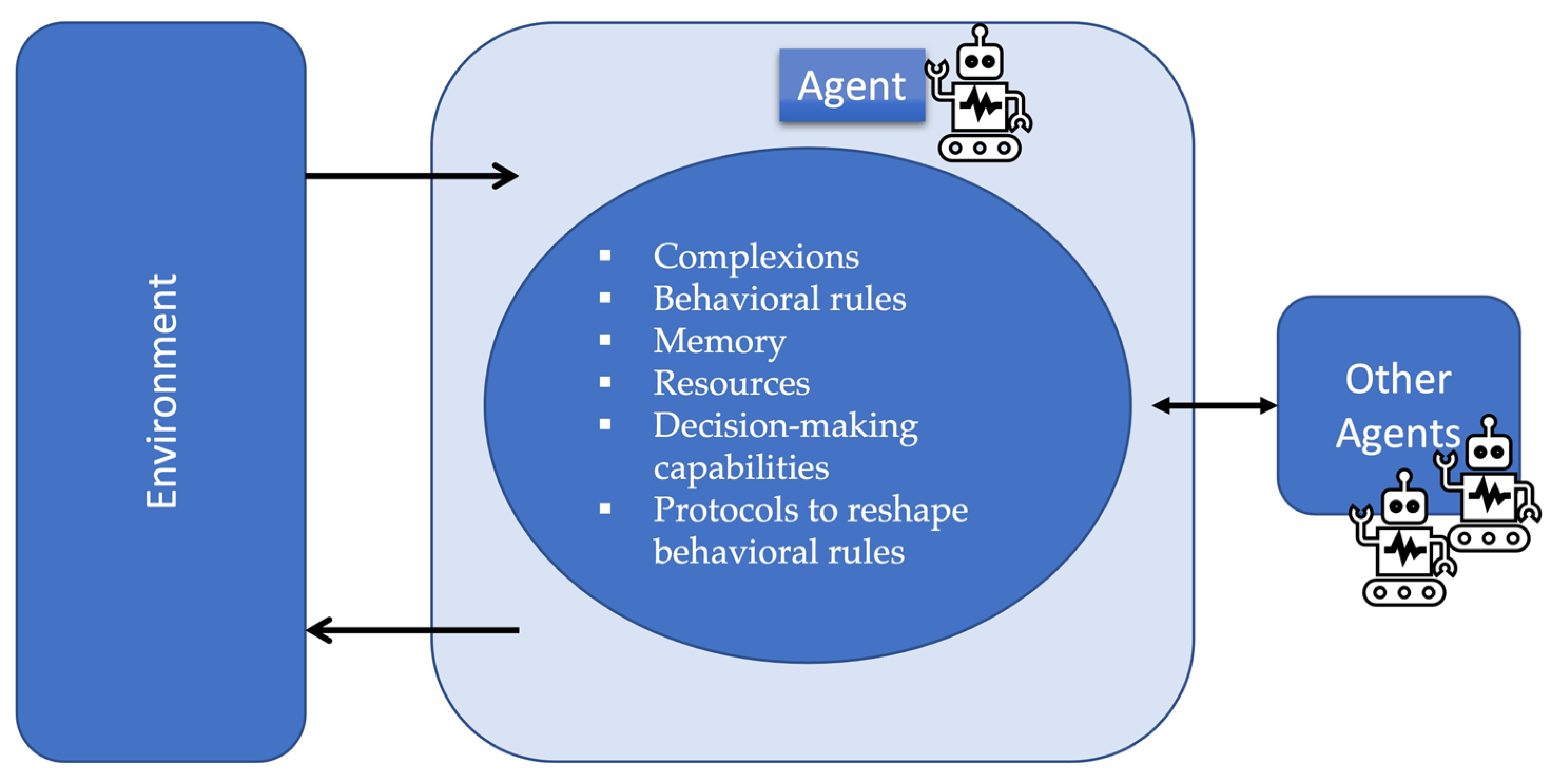
2.1. A Briefing on Agent-Based Modeling

This section provides a brief overview of ABM’s origins and its descriptive settings within challenging domains. It is important to note that some researchers [20,21,22,23] argue that ABM is a cognitive computing scheme that originated within computer science (CS) and artificial intelligence (AI). It can display prototypes, such as “single-agent systems”, in the same manner as intelligent companions and service robots [24]. This modeling technique enables a modeler to input various types of data, such as numerical and geographical data, and to create rules for the behavior of each agent. The agents can then manage perceptible environments using a model of the world (as seen in Figure 1). This approach allows for the computational modeling of social, economic, and physical processes. The agent monitors its internal state, which changes with each perception and depends on past perceptual information.

Computer simulation programs, known as ABMs, have been developed to represent the behavior and communication of agents with some level of autonomy while assessing their interdependence on a system. These programs utilize various computer simulation paradigms and techniques. Due to the vastness of the ABM paradigm, this paper will not provide a detailed description. Still, some fields in which its paradigms are widely applied are found in the institutional and commercial, economic, infrastructure, and displacement of individuals [25,26], as well as fields like biology, ecology, and social science [27]. Therefore, readers are also encouraged to familiarize themselves with the relevant literature [28,29,30,31,32].

Figure 1. Depiction of a distinctive agent within the ABM framework for streamflow simulation. The figure illustrates the agent’s interactions with its surroundings, represented by arrows pointing to and from the environment. Additionally, the figure shows the agent’s interactions with other agents in the system, as indicated by arrows. These interactions demonstrate the dynamic exchange of information and influence between the agent, its environment, and other agents, highlighting the complexity and interconnectedness of the simulation framework. Modified from [28].

Figure 1. Depiction of a distinctive agent within the ABM framework for streamflow simulation. The figure illustrates the agent’s interactions with its surroundings, represented by arrows pointing to and from the environment. Additionally, the figure shows the agent’s interactions with other agents in the system, as indicated by arrows. These interactions demonstrate the dynamic exchange of information and influence between the agent, its environment, and other agents, highlighting the complexity and interconnectedness of the simulation framework. Modified from [28].

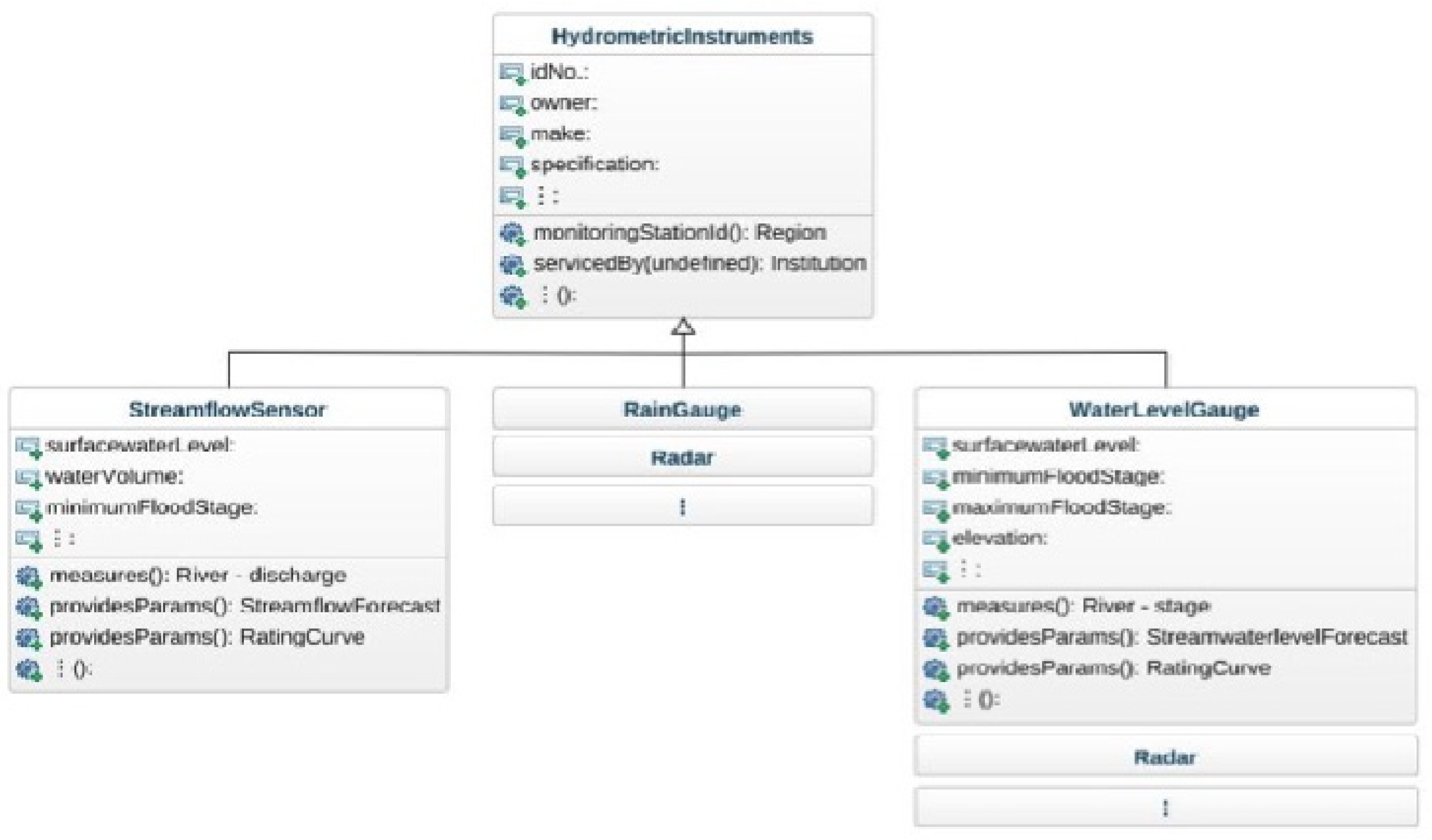
2.1.1. Domain Model Ontology

The programming of agents in an agent-based modeling domain follows an object-oriented modeling approach. In this context, a domain ontology describes the agents involved, the numerous pieces that comprise a specific modeling domain, and the relationships between these elements. An ontology for the phenomena under examination should clearly define the key concepts, attributes, and relationships relevant to the framework, considering any limitations, norms, and boundaries relevant to the study.

The goal here was not to implement an ontology related to river flow simulation within the scope of a non-hydrologic model prototype; however, it should be noted that creating an ontology is a labor-intensive engineering task. However, several development processes have been documented in various works [33,34,35,36] to assist with the creation process, including their implementation, testing, validation, recycling, and maintenance until delivery, as design approaches and guidelines. Since none of the provided recommendations is standard, the ontology implementer can use any strategy (e.g., domain-specific ontologies, upper ontologies, application-specific ontologies, and hybrid ontologies), even a mix of them, or whatever is reasonable for the domain ontology [37,38]. Despite being classified as taxonomies and vocabularies, ontologies’ primary function is the request-driven exchange and reuse of knowledge. This implies that ontologies may describe the subjects and relationships in a given domain, which can subsequently be shared and utilized by intelligent agents and their end users [39]. Sharing and reusing ontologies requires understanding the domain concepts, needs, details, and connectivity of the model designs developed for each agent and subsystem comprising the domain of study [40]. As a result, the ontology should be domain-specific to allow knowledge transfer, recycling, and redistribution. Subsequently, it was determined to leverage several of the pre-existing flood taxonomies discovered previously in the literature, such as those implemented in [41,42,43], to modify and match domain terminologies and extract the usual basic information that reflects the classes important to streamflow simulations, as they contained favorable hydrological, hydraulics, and sensor network principles.

When simulating streamflow, hydrometric equipment is required to track the factors attributed to the flood phenomenon and its prognosis, as depicted in Figure 2, which shows the Hydrometric Instruments Category. Hydrologic data collection and monitoring are essential when studying and comprehending climatic events to implement models that describe the rainfall-runoff process. Consequently, Streamflow Sensors, Rain Gauges, Rain Radars, and Water Level Gauges or Radars are a few examples of hydrometric instrumentation.

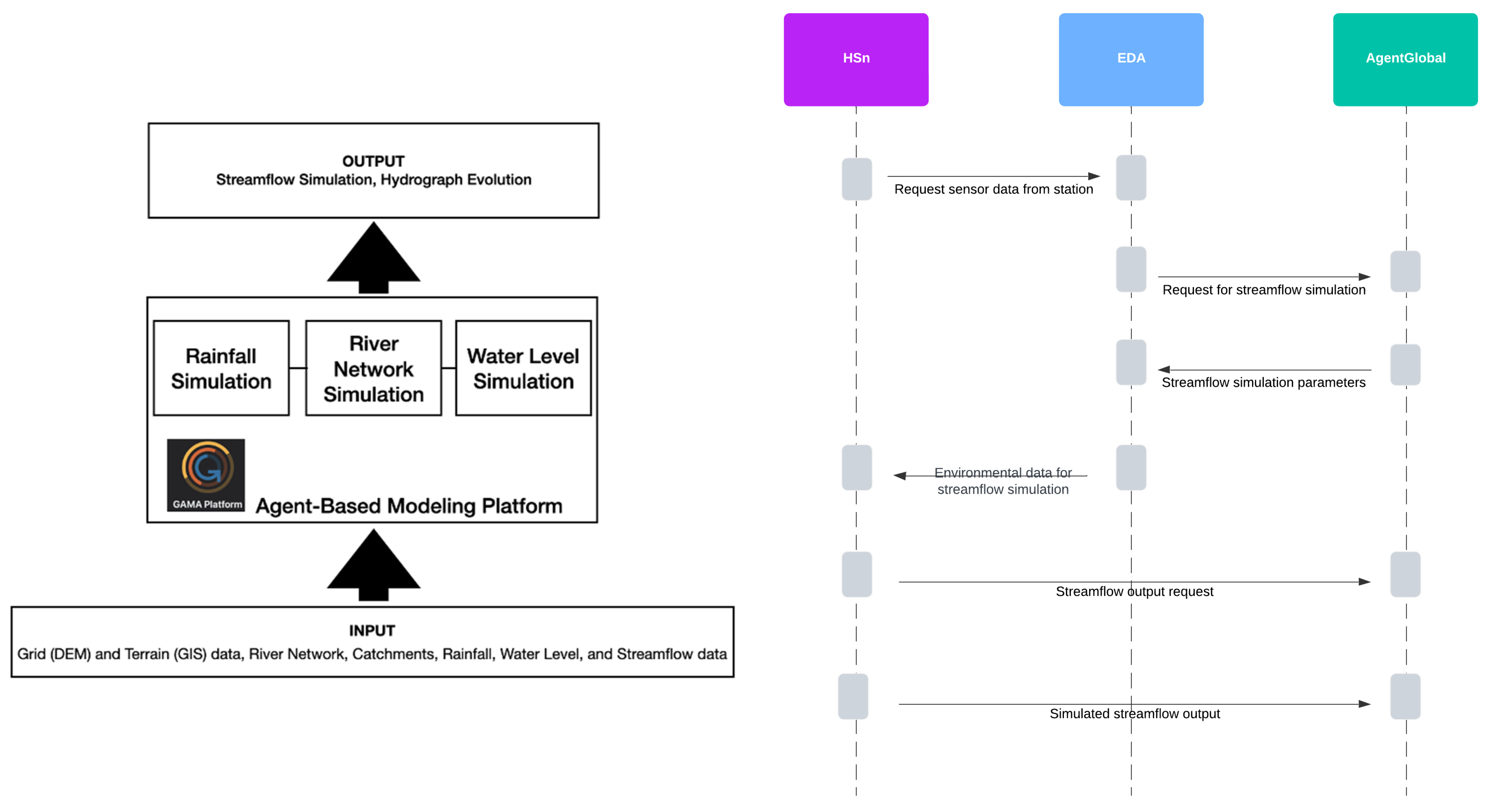
2.1.2. ABM Framework for Flow Simulation

The framework considered for designing and developing an ABM computational tool to simulate hydrologic flow scenarios to evaluate the consequences of critical flood surges is complex. To ensure the thoroughness of our research, we have chosen to follow the methodology presented by Magid et al. [44]. This methodology, with its meticulous analysis of procedures and development of the organizational structure for each agent’s behavior, is a testament to our confidence in the approach, for example, how it is structured in the GAMA platform [45].

While many agent-based development platforms for deploying agent-based simulations did not elaborate on the proposed ABM for hydrologic flow simulation, our search led us to the Generic Agent-Based Modeling Architecture (GAMA) platform [46]. With its potential for both micro- and macro-model simulations, GIS orientation, and the feasibility of implementing the BDI model, this platform stands out as a unique and innovative tool for our research.

The overall setup of the agents conveys an arrangement in which agents can be connected to the deployed hydrometric sensor network or a database. The agents fetch knowledge of the physical conditions of the river’s reach through the sensors it links them to (e.g., rainfall, surface water elevation, and discharge sensors). As several options are available for implementing this system, few other platforms specifically offer the capabilities of the “agentification” of the catchment components, such as GAMA. A schematic illustration is provided in Figure 3, which illustrates the main idea for the flow of information among the agents and their roles defined in Section 4. The GAMA platform has been in development since 2007 by the “MSI research team”, whose headquarters is situated at the “Institut de la Francophonie pour l’Informatique (IFI) in Hanoi”, which is part of the Programme Doctoral International (IRD) and the UPMC which is an International Research Unit (UMMISCO) [45].

2.2. Some Applications of ABM in Streamflow Simulation

Current research in agent-based modeling (ABM) lacks comprehensive literature [47] on using ABM to address hazards caused by hydrological phenomena. However, the following paragraphs will briefly overview articles that discuss the use of ABM paradigms and other methods to address hydrological issues, even though they may not be exclusively related to streamflow simulation.

In a study, Brouwers and Boman [48] implemented a single agent-based model (ABM) to understand people’s preferences for evaluating flood management plans in communities with spatial expansion using a geographically specific flood simulation model. Anantsuksomsri and Tontisirin [49] reviewed agent-based modeling (ABM) applied to disaster management. In their review, they explain the development of such systems, define ABM, and provide insights into some software toolkits used for building ABM systems. Coates et al. [50] used geospatial systems and agent-based modeling (ABM) to identify flood-prone commercial properties and improve flood occurrence modeling. They also recommended creating prototypes to enhance business continuity during and after flood events.

Berglund’s [51] research explored the use of agent-based modeling (ABM) in the water industry, outlining its potential and limitations in simulating planning issues related to water supplies.

Yang et al. [52] created an agent-based model to help homeowners prepare for floods. Agents simulate how homeowners react to a flood and assess potential damage. They considered factors like estate value and warning communication to decide response processes. The model found that floodplain areas and densely populated regions are more vulnerable to damage and that the ABM is useful for evaluating home losses and responses to storms.

Condro and Widagdo Condro and Widagdo [53] developed a process-based model using land cover, weather, and soil properties to explain hydrological dynamics. Following topography patches, the model clarified the surface water distribution and accurately matched the field observation data. Shirvani et al. [54] developed FLAMEGPU, a simulator for modeling interactions between flooding and people. It uses agent-based information exchange and behavioral rules for pedestrians in floodwaters. Demonstrated in a flooded shopping center, the simulator optimized barrier height and responder numbers for safe evacuation and pre-flood sandbag deployment. Huber et al. [55] created “AquaMORE”, an environmentally friendly water use platform. It models resource flows in “human-water” systems, simulating the dynamics of water resources in a demand and supply system through individual agents and feedback loops. Farias et al. [56] investigated water resources in watersheds using the agent-based modeling GAMA platform. They modeled two regional river basins by treating areas and tributaries as agents, allowing water to flow between adjacent regions. This approach, which combines pedestrian and hydrodynamic models, has garnered significant research attention and has been the focus of several publications.

In the literature review, it is evident that while there have been efforts to utilize agent-based modeling in addressing water resource issues, the focus has mainly been on applying the theory of agents, sometimes in combination with hydrodynamic models, to simulate human responses to floods rather than specifically for streamflow simulation. This study aims to address the gaps in current research by developing specific agent-based procedures for simulating streamflow independently, without the need for coupling with hydrologic models. The existing literature often couples agent-based and hydrodynamic models to simulate flood responses. This approach is yet to be tailored for streamflow simulation. Therefore, this study seeks to explore agent-based procedures for simulating streamflow without relying on hydrologic modeling platforms. This study also intends to fill this gap by providing dedicated agent-based models for streamflow simulation.

3. Materials and Methods

3.1. Study Area

The Medio River sub-catchment, approximately stretched between 08°49′58.7532″ N and 80°40′6.87″ W and 08°57′29.8188″ N and 80°40′24.049″ W, is the region that was used in this study for stream flow modeling (Figure 4), an area located within the footprint of the Mina de Cobre Panamá, owned by Minera Panama S.A. (MPSA) in the Republic of Panama, which is a component of the significant Caimito River basin. About 7 km from the Caribbean shore, it runs predominantly north until it combines with other tributaries to form the Caimito River. Currently, a sizable copper mine project exists in the upper sub-basin. The length of the Medio River from its source to its outflow into the Caimito River is about 13,800 km, and it covers a drainage area of about 50.1 km². The highest elevation is at 353.3 m, and the mean and lowest points are about 103.8 and 40.5 m above sea level, respectively. The average slope of the whole area is 51%. In the area of study, the streams are classified based on their size, ranging from small first-order streams to more significant seventh-order streams Strahler Strahler [57]. The hydrological simulation relied on the utilization of various ground-based hydrological data sources (e.g., rainfall, water level, and river flow at 15 min and 1 h spans). The information was gathered between 31 March 2012, and 31 December 2016. The Donoso region’s long-term local weather stations, associated with the average yearly precipitation, are listed in

Table 1. Average yearly rainfall in the Donoso area, Panama. Source: MPSA [58].

Observation Points	Period	No. Annual Records	Approximate Distance from the Coast [km]	Altitude [m.a.s.l]	Average Yearly Precipitation [mm]
Cocle del Norte	1966–Sep 2008	43	0.0	2.0	4989
San Lucas	1966–2008	43	10.0	30.0	4716
Boca de Toabré	1966–2008	43	20.0	30.0	4413
Coclesito	1966–1998	33	30.0	60.0	3171
Station H3	2012–2016	5	16.0	89.0	1151
Station H4 1	2012–2016	5	9.4	44.0	-

¹ No further computations were concluded due to severe record imbalance.

. The current observation points, known as Hydro-Stations (H3 and H4), are situated at the upper and lower reaches of the Medio River sub-catchment, respectively, at latitudes of 08°52′07.2″ N and 80°39′57.1″ W and 08°55′58.0″ N and 80°40′07.6″ W, with both stations covering a drainage area of about 15 and 40.4 km² respectively.

The stations H3 and H4 were both set up in early March 2012; they are both very young and have a short history of hydrologic data. However, except for the case of station H4, for which data were severely impaired, only information for station H3 is included in the tables below. As a result of this information, the Donoso region’s mean annual rainfall ranges from about 3200 mm farther inland to 5000 mm near the seashore.

Table 2. Excessive yearly rainfall in the Donoso area, Panama. Source: MPSA [58].

Return Period	Yearly Precipitation [mm]
	Cocle del Norte	San Lucas	Boca de Toabré	Coclesito	Station H3	Station H4 2
Number Years of Record	33	40	39	33	5	5
Highest Recorded	8836	6715	6239	5195	1406	-
Average	4989	4716	4416	3171	1151	-
Lowest Recorded	3164	3420	2990	2491	864	-

² No further computations were concluded due to severe record imbalance.

displays the yearly rainfall quantities related to extremely wet and dry circumstances. Stations can also collect data on conductivity, temperature, and turbidity.

3.2. Soil Type Description

The soil categorization types determine the different hydro-soil groups, which is crucial for estimating the infiltration and runoff rates at the catchment size. There is a defined infiltration rate for each soil profile. While the bottom half of the catchment comprises flat plains with gentle slopes, the upstream portion of the Medio River sub-catchment is hilly and has steep terrain. According to Mockus Mockus [59], haplic nitisols, acrisols, and vitric andosols comprise most of the catchment’s soil types. The soil of this entire catchment region contains a significant proportion of clay, which is made up of several combinations (such as “clay loam”, “sandy clay loam”, and “sandy loam”). As adopted, the different soil types in the catchments [60] are displayed in

Table 3. Medio River soil composition. Source: FAO-HWSD [60].

	Major Type of Soil Inclusions and Associated Soils
Grade	1	2	3
Land-Categories (FAO 90)	Haplic Nitosols	Haplic Acrisols	Vitric Andisols
Highland Granule	Medium	Medium	Medium
Depth of Land Source (cm)	100	100	100
Type of Catchment (0–0.5% slope)	Moderately Well	Moderately Well	Moderately Well
HIGHLAND (“Sand Fraction”) (%)	45	48	66
HIGHLAND (“Silt Fraction”) (%)	24	23	29
HIGHLAND (“Clay Fraction”) (%)	31	29	5
HIGHLAND “USDA” Granule Categories	clay loam	sandy clay loam	sandy loam

.

3.3. Land Use Description

Evergreen broadleaf forests and densely forested areas dominate the western and northern portions of the catchment basin, with some agriculture in the further northern regions. The eastern and southern-eastern zones of the catchment are distinct from the distribution of wooded savannas and grasslands, with some mining sector development. There are additional permanent marshes on the southeastern side.

3.4. Rainfall Data Description

As shown by the voids in Figure 5, the short hydrologic data observations of the two monitoring stations, H3 and H4, which comprise the rainfall data for the Medio River watershed, had several instances of missingness in the series. In any case, station H4′s statistics were far worse than station H3′s; therefore, the decision to use station H3′s data was made only for this model implementation. It is well known that issues with missing values and data gaps can occur for a variety of reasons, such as inconsistencies, inaccurate timestamp recording, duplicate records, data leakage, station sabotage (as was the case with station H4 downstream), and equipment breakdown, among others. With that said, these issues constitute the variables that obstruct the accurate management and assessment of water. As a result, the lack of standardized and complete hydrologic data information may result in the loss of significant and essential data for implementing decision-making tools for preventing floods and mitigation in particularly susceptible areas, in addition to carrying out hydrological process models at any water level of hydraulic work planning and construction.

Rainfall Distribution

Figure 6 presents the average monthly precipitation for five years of record at station H3. February and March are the driest months, with an average of about 63 to 74 mm of rain. The other months are characterized by stable moderate to high rainfall, with the highest rainfall typically occurring in November and December (93 to 182 mm).

Approximately 3.8% of the annual rainfall occurs in February and March, while the precipitation of the other months contributes between 6.2 and 24.0% of the yearly total (Figure 6).

3.5. Streamflow and Water Level Data Description

Most of the Medio River water input during the dry season comes from the base flow; however, the sub-catchment has a flow and water-level regime where rainfall is predominant. Most rain falls between May and November, although the wettest months are September and October. Because of “El Niño/Niña-Southern Oscillation (ENSO)” effects, in addition to climatic factors, including flash floods brought on by mesoscale convective systems, tropical cyclones, and frontal systems, monthly streamflow, and the resulting water level can vary depending on the hydrological regime of a year [61]. Nevertheless, river flooding primarily occurs during the rainy season, manifesting as heavy downpours, storms, and sudden floods. There are not sufficient immediate hydrometric measurements that cover the Medio River watershed despite the simulation utilizing precipitation observations. As a result, station H3 upstream of the watershed, namely in sub-catchment-4, and station H4 downriver, at sub-catchment-6, since they were the two hydrometric stations that provided the sole data for retrieval. The datasets at station H4 were determined to be partial and degraded, as previously noted in the text. The station H3 dataset is the only one with usable data, although it had some missing observations. Station H3 captured the first data on 31 March 2012; the most recent data were accessible in 2016. Station H3 files cover about five years. The hydrograph and water level show gaps in the raw dataset, as shown in Figure 5. The time series for Station H3 had to be reconstructed using data imputation techniques, which are covered comprehensively in Section 3.6, which is crucial to note for simulating flows in the catchment.

3.5.1. Water Level

During the simulation runs, the river water levels at station H3 were observed to be highly responsive to rainfall, with rapid increases occurring during or immediately after rain, followed by a rapid return to pre-rain levels. Such a response is typical of well-drained catchments with few or no significant water bodies and few appreciable floodplains to attenuate flows following precipitation events.

3.5.2. Streamflow Distribution

Table 4. Distribution of monthly and annual streamflow [m³/s] characteristics at Station H3 for the Study Area.

Hydrologic Year (HY)	Jan	Feb	Mar	Apr	May	Jun	Jul	Aug	Sep	Oct	Nov	Dec
2012	-	-	38.8	84.1	104.0	55.5	159.1	60.1	115.5	103.1	729.5	364.4
2013	75	72	94.1	50.4	102.3	89.6	79.6	50.5	63.5	82.9	75.9	183.9
2014	98	32	60.0	170.7	166.8	109.6	139.2	96.9	94.6	104.1	102.1	102.1
2015	158	75	30.6	143.1	268.8	296.7	128.2	94.1	104.9	97.0	157.3	39.3
2016	41	22	24.9	31.2	135.6	57.2	137.2	108.8	67.7	56.7	197.7	147.3
Mean Monthly Streamflow for 5 Years of Record	93.2	50.1	49.7	95.9	155.5	121.7	128.6	82.1	89.2	88.8	252.5	167.4
Standard Deviation	48.9	27.2	28.2	59.6	68.6	100.4	29.7	25.3	22.8	19.8	270.8	122.6
Maximum Flow	157.7	75.0	94.1	170.7	268.8	296.7	159.1	108.8	115.5	104.1	729.5	364.4
Minimum Flow	41.5	21.5	24.9	31.2	102.3	55.5	79.6	50.5	63.5	56.7	75.9	39.3

summarizes the monthly and annual flow characteristics, and Figure 7 shows the monthly and yearly streamflow for the H3 station for five years of hydrologic data.

From the summary displayed in Table 4, the simple statistics on monthly data for the five years suggest that monthly stream flow in the Medio River area is expected to follow the same pattern as rainfall, e.g., lower flows occurring in February and March (coincident with low rainfall), with the highest flows in November and December (coincident with high rainfall).

3.6. Hydrologic Record Reconstruction

In several domains, such as engineering, culture, psychology, and healthcare., missing data problems can be encountered. For years, academics have employed creative techniques to change the data by excluding bad instances or entering the blanks. However, hardly all of these techniques will be useful on a specific dataset, particularly across tropical catchments; established and more straightforward ways to cope with the hydrologic dataset absence and shortage remain crucial [62] due to various factors such as logistical challenges, sensor maintenance problems in harsh weather, and political and economic limitations can impact the choice and effectiveness of imputation methods. Furthermore, insufficient hydro-data, alongside concerns about flow destruction and risk evaluation, are significant issues for the administration of water resources projects [62]. Then, as a correct estimate of incomplete hydrologic datasets is essential in decision support processes for the successful management of water resources and long-term planning of water-borne systems, streamflow simulation, and flood forecasting would depend heavily on this information [62]. Unfortunately, many of these methods are biased and call for a rigid assumption regarding the reasons for missing data. Although these techniques are becoming less and less prevalent in the methodological literature [63,64], they are nevertheless widely used in research works that have been published [65,66]. Rubin Rubin [67] defined three common missingness mechanisms: The term “missing completely at random” (MCAR) refers to situations in which instances with missing data may be seen as a random sample of all the cases. Based on the information we have available, “missing at random” (MAR) states that any missingness that remains is entirely random and does not depend on any missing factors. Where neither MCAR nor MAR seems to apply to the data, missingness may be reproduced using the observed data and missing not at random (MNAR). This is not easy to deal with since it will necessitate making significant assumptions about the patterns of missingness. Despite several data imputation techniques, multiple imputations (MI) are increasingly employed in hydrological research to deal with missing data [68,69,70,71]. This improves the precision and reliability of hydrological models and assessments. MI allows you to evaluate the uncertainty caused by missing data by constructing multiple complete datasets, analyzing them individually, and then combining the results to obtain estimates that account for the uncertainty associated with the imputation process. Any of the three types of data gap situations are manageable with multiple imputation (MI) techniques. However, MNAR instances are typically not supported by MI package designs due to their complex process. To deal with the missing instances, it is assumed that the data were missing information dependent on unobserved predictors rather than MAR; therefore, the MI technique is chosen.

Table 5. Hydrologic station H3 records with observed missing data totals.

		Variable		No. of Variables with Missing Data
No. of Instances	RN [mm]	Q [m3/s]	WL [m]
147,086	1	1	1	0
95	0	1	1	1
2977	1	1	0	1
2579	1	0	1	1
5778	1	0	0	2
8241	0	0	0	3
Total of missing	8336	16,598	16,996	41,930

Key: 1 = variable with observed data; 0 = variable with observed missing data.

displays the overall missing pattern of the data record before the imputation and model runs.

According to Table 5, 147,086 instances out of 166,756 cases were complete. Only rainfall (RN) data were absent for 95 instances, 8241 cases were ultimately missing for all three variables, and 5778 instances included only RN data. Although 88.2% of the samples were intact, water level (WL) and streamflow data (Q), which accounted for nearly 20% of the missing instances, were the variables with the most significant absence of values. Overall, the proportion of missing data for each variable out of the total cases was 5.0% for RN and 20.2% for both WL and Q, respectively. It is important to understand that ignoring missing data may not be the best approach to handling these cases. Doing so could decrease the statistical accuracy of the models being used, cause incorrect parameter estimation, and result in inaccurate findings related to the studied topic [72].

Data Reconstruction Results

In this experiment, the “Mice package”, presented in the statistical programming language R [73], was used to reconstruct the hydrologic record series by imputing the missing data. The multiple imputation method was carried out using three of the built-in univariate imputation approaches: “predictive mean matching” (pmm), “bayesian linear regression” (norm), and “non-Bayesian linear regression” (norm. nob). A detailed discussion of these functions can be found in [74]. The variables for the one-hour rainfall, discharge, and water surface elevation are denoted by the labels RN [mm], Q [m³/s], and WL [m]. The original raw dataset, which included missing instances, was reconstructed by imputing for the RN, WL, and Q variables, using the three imputation methods mentioned above; however, the best imputation results were obtained with the “pmm” imputation technique (Figure 8), and these results were chosen following the Mice package’s methodology and used as complete inputs to the agent-based model structure for hydrologic streamflow simulation. For the imputing procedure, the MICE settings can be adjusted for (e.g., number of imputations = 10, iterations = 50, and seed = 500), and the three imputation algorithms are selected. For each variable with incomplete instances, the MICE package can also assist in selecting the collection of indicators that should be utilized in the imputation procedure. The selected pmm algorithm yielded an adjusted R² (0.8524) by modeling the imputed datasets and merging the results. A summary of this model’s fit also indicated that the predictors RN and WL significantly impacted the response variable Q, with p(=0.00). There is a significant interaction between the two predictor variables due to the relationship between the predictor rain and the response variable (discharge), which depends on the level of the predictor of water surface elevation. As a result, the equation WL(t) = 8.23 + 0.0018RN(t) + 0.020Q(t) is obtained as the imputation model for predicting the WL(t).

4. ABM Experimental Setting

4.1. Hydrologic Information Extraction

This experiment used the resulting corrected hydrologic record of 1-h rainfall, water level, and discharge data from Section 4.3 as input data for the ABM model setup to simulate hourly streamflow from selected single storm events, as shown in the next section.

4.2. Storm Episode Selection

This section explains the goal for identifying the intervals in the hydrologic data series that reflected situations involving rainstorm events that might be utilized to simulate and predict flows using the agent-based modeling paradigm; hence, the historically reconstructed hydrologic time-series data that correlated to a flood event were necessary (Figure 9) for observing the river water level and hydrograph’s severe flows (“rating curve” in Figure 10) on station H3 flow rate. As a result, the focus was on the months of each year that had significant rainfall events, which were selected and utilized for calibration and model tuning.

From this perspective, selecting the times during which a specific storm was helpful in model calibration (selected maximum matching days of high precipitation) was crucial for looking for periods in the series that showed an improved trend in rainfall and streamflow. This was achieved by plotting historical data on rainfall and streamflow and looking for unusual peaks, bearing in mind that a peak in the rainfall data may or may not correspond to a rise in the streamflow. Even though heavy precipitation can trigger flooding and cause an increase in stream flow, stream flow measurements are a more reliable indicator of potential rainstorms compared to rainfall alone. This is because heavy downpours may only sometimes cause flooding. Whenever there is a significant increase in a river’s streamflow, it is widely known that this can lead to the river overflowing and causing an inundation.

Multiple criteria are used to identify critical rainfall, such as those reported by Jang [75], Blanc, Hall Blanc, Hall [76], Cheng, Li Cheng, Li [77], Hurford, Parker Hurford, Parker [78], and Priest, Parker Priest, Parker [79], according to the “International Meteorological Vocabulary”, heavy rain is defined as accumulating precipitation with a depth ratio of more than “7.6 mm · h⁻¹” [80]. The “Canadian Atmospheric Environment Service” defines intense storms in the Americas as rain occurrences that surpass a cut-off value of >25 mm·h⁻¹ [81]. In places like Indonesia, a tropical nation with a pattern of yearly precipitation akin to that of the Isthmus of Panama, the “Badan Meteorologi Klimatologi dan Geofisika (BMKG Sofiati and Nurlatifah Sofiati and Nurlatifah [82])” proposed a class one and class two acute rainfall limit, with classification one being the upper limit for “daily operational definition of precipitation (DODRE)” the maximum for class two being the “monthly operational definitions of precipitation events (MODRE)”, according to

Table 6. Limits of acute rainfall quantity. Source: [82].

Classification of Precipitation	Rainfall Quantity
	Classification I [mm·h−1]	Classification II [mm·d−1]
Light precipitation	1–5	5–20
Average precipitation	5–10	20–50
Intense precipitation	10–20	50–100
Very intense precipitation	>20	>100

below.

In the hydrological sciences, it is common practice to distinguish intervals of rainfall recesses between discrete rainfall events that last longer than a certain amount of time or the “inter-event time” (T_i) intervals of rainfall recesses between discrete rainfall events that last longer than a predetermined amount of time, or the “inter-event time of the spaces” depicted on a hyetograph. Nonetheless, in the literature, Field has proposed several criteria for isolating rainstorms using defined “Inter-Event” durations ranging from 3 min to 24 h [83,84]. In this model makeup, the autocorrelation function time in the rainfall data led to selecting an inter-event time of T_i = 2 h.

The time series are subjected to the Pearson correlation coefficient analysis to calculate the lag time for the overall rainfall series and the single months chosen. Figure 11 displays a rough estimate of the autocorrelation function for all periods of the H3 station, with time lags varying from 1 to 4 h. This conclusion was drawn for each month the rain data were evaluated. Hence, T_i = 2 h was chosen as the suitable lag time for the rainfall series. Not every time there is a storm, there will be flooding, and not every storm will result in floods. Identifying peaks in the streamflow data that correspond to a flood must comply with additional rules or requirements in addition to those indicated in the previous paragraphs when periods with significant flood episodes are chosen. Since the most current rating curve from the whole series must be used in simulations, the data must first be reduced. Then, to identify which streamflow data peaks correspond to floods, the following directives are applied:

1.

Storm Depth: The storms under consideration must be so intense as to cause flooding. However, because genuine hydro-records are now sparse, knowledge that might correlate precise streamflow data to the timing of a future flood might be challenging to acquire; so, it is assumed that only the documented maximum heights produced floodwaters.

2.

Storm Duration:

• For a downpour to be replicated as a storm event, it must be visible in the hydrologic dataset.
• Preceding and antecedent flow conditions must be sufficiently low to be assigned to the base flow during these times, disregarding the antecedent soil moisture.
• The extent of flood days is verified using residents’ and precipitation records.

3.

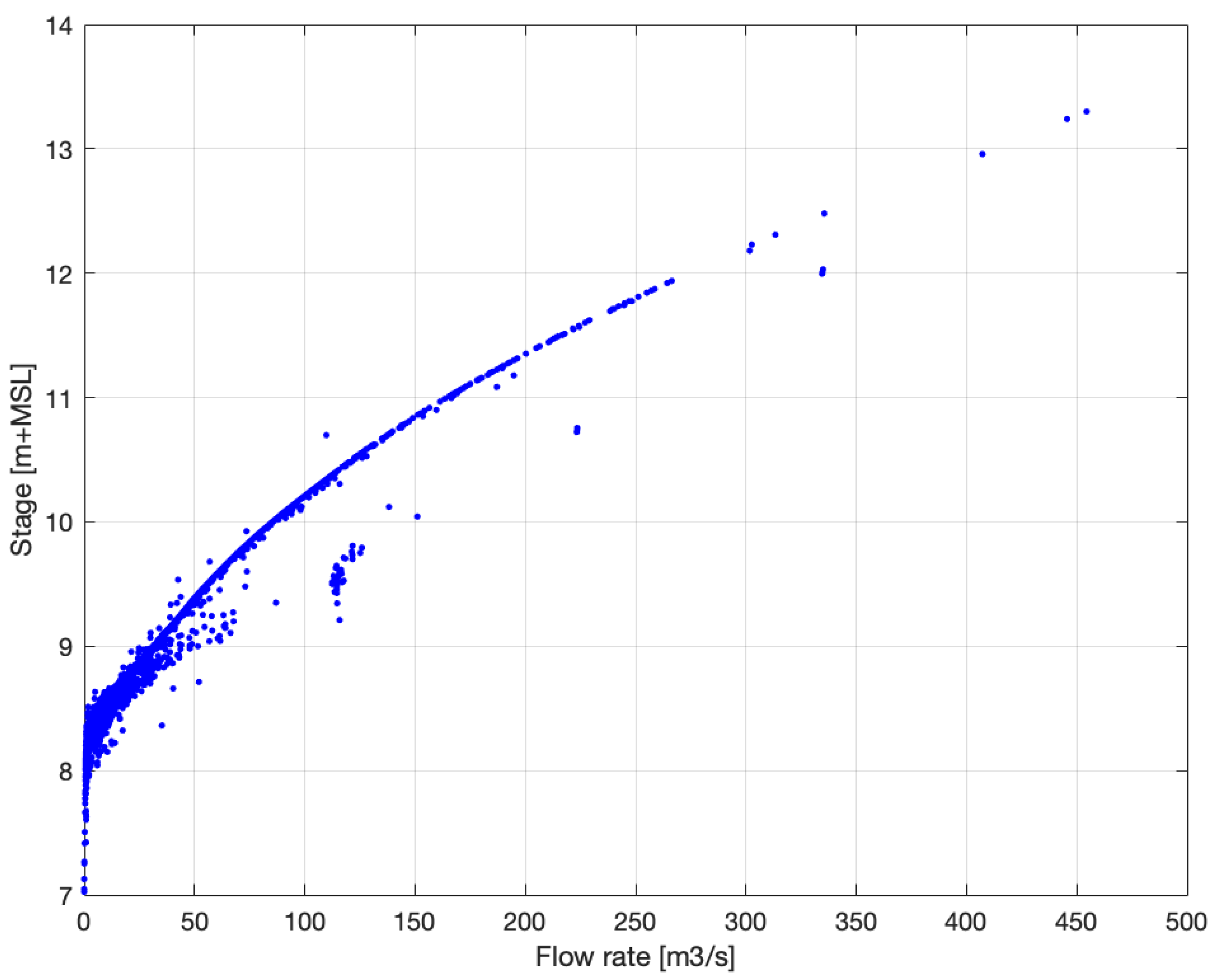
Storm Period: Using the given data, linking storms to the computed rating curve shown in Figure 10 should be possible. This ensures that the modeling approach is accurate and matches the river’s present hydraulics (i.e., channel shape).

4.

Data Accuracy: Because the hydrologic database stores all its data electronically, outliers, inconsistent records, data gaps, and missing values can produce errors in the results. Therefore, each instance of the hydrograph should be related to the dynamics of active physical processes.

Although the storm depth peaks can be observed using the information in Figure 6, selecting them is a challenging assignment (Directive 1). It was, therefore, crucial to trim the data, plot the separated hydrographs, and choose the various peaks corresponding to intense storm episodes (Directives 1 and 2 (points 1 and 2)). In addition, the details shown in the previous figure’s hyetograph immediately reveal several storm events, of which at least fourteen were extracted for their hydrological analysis and assessment. Still, five were relevant, which is why they were selected during the preparation of this experiment.

The individual hydrographs observed in Figure 9 offer an overall understanding of the rainstorm and flood peaks in the data record, enabling us to select whether among these flow surges equates to an actual overflow and consider whichever of them to employ in setting up for the hydrologic simulation. However, deciding can be difficult, as indicated by the graphs; there are localized rapid floods, often brought by heavy rain (i.e., flash floods), another critical factor that can be noticed. With the latter said, the December 2013, September 2014, May, and December 2016 rainstorms went unnoticed using this methodology since they did not meet the provided parameters 1 and 2. Despite appearing high in the graphs, each of these rainstorms’ peak streamflow rates did not produce enough flow time to guarantee a flood (Directive 2). Moreover, streamflow rates rapidly decreased at the height of precipitation, probably due to flash floods.

On the other hand, the data for the streamflow and rainfall for the storms that occurred in May and November 2015, December 2014, and November and December 2012 were examined. (Directives 1, 2, and 4, respectively) and separated for the entire simulation task.

Then, the selected months for each storm episode (Figure 12, Figure 13 and Figure 14) show the daily correlation between each month’s rainfall and streamflow data throughout the year with a specific rainstorm event. Additionally, it is possible to spot shifting patterns in the graphs, where specific trends are predictable, but others are perplexing. This exemplifies how intricately connected some of the fundamental processes of the water cycle are. This results in a highly diverse reaction of the Medio River to rainfall, as revealed by a thorough analysis of several sectors of the overall charts.

As we observe Figure 12, Figure 13 and Figure 14, it can be noted that during the rainy event that began on 1 November, the precipitation increased gradually from 26 mm to 94 mm before decreasing to approximately 10 mm on day 14th. This precipitation was followed on the 11th by a slight increase in river discharge, and there appears to be a fluctuating pattern of about 2.5 and 105.7 m³/s. Nonetheless, the largest per hour rainfall observed was 170 mm on days 18th through 22nd, with an observed stream flow of 227.4 m³/s; however, the less intense per hour rainfall occurrence of days 24th through 26th is noteworthy, with a more significant rise in the flow of the river of 258.6 m³/s.

Like the rainfall in November 2012, two reported high flows in the river are defined by the hourly rainstorms in December 2012 and the associated streamflow profiles, which might show that the period’s data are consistent with the measured rainfall reported at that time. The rise in streamflow is related to the increase in precipitation, and like the November 2012 storms, the same patterns, whereby a less intense rainfall event causes a more significant amount of discharge into the stream than a more extraordinary rainstorm occurrence, may be observed. There were three stormy occasions in December 2014, with the events of the 7th through 12th and 13th through 15th being so far prominent. During this time, streamflow increases for both rainstorm events, and as was previously demonstrated, there is a similar discrepancy with rainfall that falls on days 11th through 14th that totals about 1498 mm but is followed by a higher water flow that amounts to 335.5 m³/s; conversely, on day 11th, yet, with 106 mm of rainfall, there is still a significantly modest rise in the stream flow of 206.2 m³/s.

During the storm of May 2015, there were two documented maxima in the flows and precipitation, the flows being 110.3 and 269.1 m³/s, and the precipitation was 40 and 39 mm recorded for the days 16th and 20th. As in past storms, precipitation and enhanced streamflow coincided; additionally, there was a more significant river discharge with shallower rainfall. The enormous daily water flow of about 264.3 m³/s and the heaviest hourly rainfall of 196 mm were recorded on the 26th of November 2015 during the storm, which occurred from the 23rd to the 30th. It was noted in the previous paragraphs that each downpour so far has shown that even a small amount of prolonged rainfall can cause a significant rise in runoff volumes. This function provides a precise image of the link between precipitation and streamflow in the Medio River basin as the stream responds to different precipitation levels. The reality that the region of the Medio River basin is in an intense precipitation zone in tropical areas and the likelihood that the hourly rainfall on any one day might surpass 25 mm·h⁻¹ are merely two of the forces that, once paired together, result in a complicated rainfall-runoff connection. The relationship between streamflow and precipitation is closely associated with several human and environmental factors. Therefore, these factors should not be overemphasized.

As previously mentioned, a few variables affect how a river channel reacts to a rainstorm event. Several of these factors will evolve across time and space inside a single catchment. For illustration:

• Rainstorm intensity

High-intensity rainstorms result in rapid runoff and increased river surface flow, potentially causing flash floods. Low-intensity rainstorms allow more water to infiltrate the soil, reducing immediate runoff and gradually increasing river flow.

• Rainstorm duration

Rainstorm duration significantly affects river behavior. Prolonged rain saturates the soil, increasing runoff, floodwater, and flooding risk. Short, intense storms cause rapid water level rise, stressing river channels.

• Air temperature

Air temperature affects how rivers respond to rain. Warmer temperatures can lead to increased evaporation, potentially reducing river water. Colder temperatures may reduce evaporation, leading to more prolonged river flow after a rainstorm.

• Wind speed

High wind speeds can quickly transport moisture, leading to uneven rainfall distribution and localized areas of intense rainfall, which affects runoff and river channels. Strong winds can also increase evaporation, reduce water, and contribute to runoff, but this effect is usually less significant than rainstorm intensity and duration.

Even so, there are still more elements to consider that may or may not change from period to period but can potentially affect the precipitation-streamflow connection. Additionally, these traits will vary from one basin to another. Some are listed below:

• Kind of soil type

Soil type determines how much precipitation is absorbed into the ground and how much runs off into streams. Soils with high permeability, such as sandy soils, allow more water to sink in, reducing immediate runoff and streamflow during rainfall. On the other hand, clayey soils, which have low permeability, cause higher surface runoff, leading to quicker and potentially more substantial streamflow responses. The soil’s ability to retain water also impacts the base flow of streams during dry periods.

• Land usage

Land use affects how water behaves in urban areas. Lots of pavements cause fast runoff. Agriculture can either help water soak in or make it run off faster. Forests are good at letting water soak in and holding onto it.

• The slope of the basin

The basin’s gradient impacts the rate and amount of water flowing into the streams. More abrupt gradients encourage swifter water flow, raising the risk of sudden floods and larger peak stream volumes. Conversely, gradual gradients impede water flow, providing additional absorption time and reducing the stream flow’s immediate effect.

• Riverbank (slope)

The riverbank slope affects water flow. Steep banks lead to fast movement and erosion, impacting stability. Gentle slopes slow water, promote sediment deposition and improve water quality.

• Channel configuration

The stream channel configuration, shape, size, and path affect the water flow. A narrow channel speeds up water transport, causing rapid streamflow during rain. A broader meandering channel slows down water, encouraging infiltration and reducing peak flows. Channel modifications like channelization or levee construction can significantly alter natural flow patterns and hydrological connectivity.

• Geospatial and climate differences

Geospatial variations, like elevation and topography, and climate differences, such as precipitation patterns and temperature, significantly influence the precipitation-streamflow relationship. Regions with high and consistent rainfall exhibit different streamflow characteristics compared to arid areas with infrequent but intense rainfall events. Elevation changes within a basin can create microclimates that affect how precipitation translates into streamflow.

• The amount of vegetation and the proportion of impervious surfaces

Plant life naturally regulates water movement by capturing rain, promoting absorption, and slowing surface water flow. In urban areas, impervious surfaces limit these benefits, increasing water flow. Additionally, plant life enhances evapotranspiration, reduces water volume, and contributes to flow.

Specific modifications and calibration of the measurable precipitation information (e.g., Bias Correction and Quality Control, Adjustment and Spatial Interpolation, and Climate and Regional Adjustment) are necessary to utilize rainstorm data in modeling effectively. Additionally, it is crucial that the data are accurate and consistent with the replicated hydrograph for the procedure to yield successful results.

The features and trends of the substantial streamflow during the storms in May and November 2015, December 2014, and November and December 2012 suggest that floods in the Medio stream most certainly occurred. According to the hydrometric records and rating curves that are currently accessible, the population in the catchment was affected by high flows. The streamflow-rainfall analysis of the actual hydrologic data demonstrates that the flooding episodes resulted from the streamflow and were caused by the noteworthy rainfall depth and streamflow rate.

4.3. ABM-Driven Streamflow Simulation

4.3.1. ABM Environment Selection

One of the motivational objectives of this model development, as shown in Figure 15, is to use the ABM paradigm environment rather than the typical hydrological archetypal software model to reproduce the simulations of hydrological flows in a tropical catchment. According to a study of an agent development platform, there are numerous platforms for creating agent-based modeling tasks in this context. Some relevant remarks discovered when researching the subject among the most popular are “NetLogo version 6.1.1”, “JADE version 4.5.0” as well as its extension “JADEX version 4.0.241”, “MACSim version 2005” [85] an API developed to enable communication with JADE 3.6.1 via MATLAB version 7.8/7.11 (R2009a/R2010b) and Simulink version 7.6, and the recent “Generic Agent-Based Modeling Architecture” (GAMA) platform [46]. Regardless of these and other options, and because many of the inputs used in this simulation rely on geographically referenced data, the “GAMA platform” was decided on as the preferred agent-based modeling environment setting for agent modeling as it enables the application of geospatial datasets as imports and the mapping of the field data, fluctuation in water quantities, visual streamflow, and river water levels. Its strong GIS orientation also enables the environment domain’s numerous configuration settings to have varied values by updating the primary code base.

The GAMA platform discretizes GIS components into distinct spatial layers and exhibits them autonomously, enabling simple and seamless communication between these layers. As a result, every sub-catchment (as shown in Figure 16a) regards the influence area (watershed) as a singular agent tied to its specific collection of features and attributes. In Figure 17a, for example, the format and location of each sub-catchment can be observed together with the color attribute added to each of them to aid in their differentiation. Through the relationship between the user’s input and the items’ geometry and location, GAMA creates updated data. Figure 16b is a depiction of the scene shown (rivers). Figure 16c (river networks and sub-catchments). This image shows that the platform can extract updated data and properties for every item, such as connecting a river to a particular sub-catchment based on its geographical position.

This section describes the ABM Medio catchment hydrologic modeling agent species (classes) in detail. These sub-catchments have been discussed under Section 3.1 and here in (Figure 17a), with the distinctive qualities and properties of the “AgentCatchment” provided as an example in

Table 7. Spatial characteristics of the AgentCatchment.

Subcatchment_ID	Area [km2]	≈Order	Catchment Outlet_ID
1	9.9	3	4
2	6.3	2	4
3	9.6	3	4
4	4.9	1	8
5	5.3	1	8
6	12.8	2	8
7	1.3	1	8

. The following agents, some of which may be categorized as static and non-static agents, comprise the model layout (Figure 18) for this agent-based two-level architecture.

• Hydrometric sensor agents (HSn): Due to technical constraints, the hydrometric station’s three sensors collect data from simulated document files. Future efforts will pursue real-time data tests.

• The role of the rainfall sensor agent (AgentRNSn) is to record, aggregate, and provide river agent sources with real-time incoming rain data readings.
• The water level sensor agent’s (AgentWLSn) job collects, aggregates, and provides the river agent with real-time incoming river surface–water level data.
• The role of the streamflow sensor agent (AgentSFSn) is to receive, aggregate, and provide the river agent with real-time inflow flow data on discharge derived from field flow meter sensor data.

For each agent described in this level, a brief description of their rules and interactions is provided below in Algorithm 1.

Algorithm 1. Hydrometric Sensor Agents (HSn). Details of the pseudocode for initializing and defining the roles of hydrometric sensor agents within the agent-based model.

1: Agent HydrometricSensor: 2: type: Rainfall, WaterLevel, Streamflow 3: data source: SimulatedDocumentFiles 4: for Every time step,… do 5:      BehaviorCollect data(): 6:      for behaviorcollect data(): do 7:    if type == Rainfall then 8:        AgentRNSn.collect rainfall data() 9:        behavior collect rainfall data(): 10:      data = read data from simulated file() 11:      aggregate data(data) 12:      provide data to river agent(data) 13:     else if type == WaterLevel: then 14:      AgentWLSn.collect water level data() 15:      behavior collect water level data(): 16:      data = read data from simulated file() 17:      aggregate data(data) 18:      provide data to river agent(data) 19:     else if type == Streamflow: then 20:      AgentSFSn.collect streamflow data() 21:      behavior collect streamflow data(): 22:      data = read data from simulated file() 23:      aggregate data(data) 24:      provide data to river agent(data) 25:    end if 26:  end for 27: end for

• Environment domain agents (EDA): The catchment environment comprises four agents in addition to the default global agent created by GAMA. See Algorithm 2 for an overview of the script.

• Catchment agent (AgentCatchment): The static agent simulates the Medio River catchment with specific parameters for the area, catchment hierarchy, nearby sub-catchments, drainage outlet, main channel, rivers, and monitoring stations. These characteristics help determine the gradient behavior of the catchment and enable interaction with the river agent for water transport and exchange.
• Water source agent (AgentSource): The hydrologic agent manages river flow by adjusting the water supply based on flow and precipitation data at the start of the simulation. Source agents are linked to river inlets and are directed to supply a predetermined quantity of water based on the input volume, flow, and precipitation data.
• River network agent (AgentRiver): The river agent is distributed among sub-catchment locations and moves water within the catchment. It calculates the volume of water in a river using information from the precipitation series. Water exchange between river reach segments in neighboring catchments is influenced by precipitation volume and frequency, resulting in flow routing. According to Neitsch [86] et al., the AgentRiver manages water flow in the river systems by computing flow rates and estimating water levels. This is achieved by overseeing the global agent and responding to the requests.
• Terrain elevation agent (AgentDEM): The “agentified” DEM is a unique form of an agent class with a grid structure. It is a static agent with no mobility during the simulation time. It represents the catchment terrain elevation and is responsible for the overall gradient profile.

Algorithm 2. Define Environment Domain Agents (EDA). Presents the pseudocode for initializing and defining the actions of the environment domain agents. These include the catchment agent, which simulates the Medio River catchment and interacts with the river agent; the water source agent, which manages river flow; the river network agent, which distributes water and calculates volumes within the catchment; and the terrain elevation agent, which represents the catchment terrain and gradient profile.

1: Agent Catchment(AgentCatchment): 2: properties: 3: area 4: hierarchy 5: sub catchments 6: drainage outlet 7: main channel 8: rivers 9: monitoring station(s) 10: for Every time step,… do 11:     behavior simulate catchment(): 12:     for behaviorSimulate catchment():,… do 13:      determine gradient behavior(): 14:      interact with river agent(): 15:     if Rainfall = 0 then 16:       Agent WaterSource(AgentSource): 17:       behavior manage water flow(): 18:       initial water supply = calculate initial supply() 19:       adjust water supply(initial water supply) 20:       no link to river inlets() 21:    end if 22:    for AgentRiverNetwork(AgentRiver): do 23:    behavior distribute water(): 24:    volume of water = calculate water volume(initial water supply) 25:    route flow between segments(volume of water) 26:    calculate waterLevel = calculate waterLevel(volume of water) 27:    waterLevel update = calculate waterLevel() 28:      if Rainfall ≥ 1 then 29:      Agent WaterSource(AgentSource): 30:      behavior manage water flow(): 31:      initial water supply = calculate initial supply() + Precipitation 32:      adjust water supply(initial water supply) 33:      link to river inlets() 34:     end if 35:    for AgentRiverNetwork(AgentRiver): do 36:      behavior distribute water(): 37:      volume of water = calculate water volume(initial water supply) 38:      route flow between segments(volume of water) 39:      calculate waterLevel = calculate waterLevel(volume of water) 40:      waterLevel update = calculate waterLevel() 41:     end for 42:    end for 43:   end for 44: end for

• Global agent (AgentGlobal): Defined in the Algorithm in Algorithm 3, the global species in GAMA is an automatically created agent representing the entire environment. It describes all variables, parameters, actions, and behaviors that regulate the world and oversees and manages all other agents within the system. It also archives the data generated during the simulations, acting as a supervisory agent.

Algorithm 3. Define Global Agent (AgentGlobal). This algorithm outlines the pseudocode for the global agent, which is an automatically created entity in the GAMA platform that represents the entire simulation environment.

1: Agent GlobalAgent(AgentGlobal): 2: properties: 3: environment variables 4: system parameters 5: for Every time step,… do 6:     behavior oversee system(): 7:    for behavioroversee system(): do 8:       regulate world variables() 9:      manage agents() 10:      archive simulation data() 11:    end for 12: End for

Since Shannon’s creation of the information theory [87] the concept of complexity has been studied even earlier. Over the past few years, the study of complexity in modeling systems has gained recognition in the statistics community. Model attributes like modeling error and sensitivity can be used to define the uncertainty of the system, which is directly linked to a model’s complexity.

As depicted in Algorithm 1, each HydrometricSensor agent collects data at every time step. Depending on the type (Rainfall, WaterLevel, Streamflow), it performs specific data collection tasks. The data are read from simulated files, aggregated, and provided to a river agent. Such a task comes with its computational complexity. In simple terms, say time complexity is Ω(T × S), where T is the number of time steps, and S is the number of hydrometric sensor agents; the time it takes for the hydrometric sensor agents to do their job depends on how many time steps there are and how many agents there are. Each agent performs tasks like reading and sharing data with the river agent during each time step. The amount of space complexity needed is Ω(S), which also depends on the number of agents, as each agent keeps track of their own data. In addition, in Algorithm 2, we observe that at every time step, every catchment agent replicates catchment behavior. It interacts with river networks and water sources to control and distribute water flow depending on the amount of rainfall. Water levels are determined and updated by catchment agents using rainfall and water supply data. This task is defined by a computational complexity expressed as Ω(T × U × P), where T is the number of time steps, U is the number of catchment agents, and P is the number of river network segments or water source interactions. Each time step involves multiple operations for managing water flow, distributing water, and updating water levels. The space complexity is then defined by Ω(U + P), as each catchment agent needs to maintain properties related to the environment domain and interact with multiple river network segments. Finally, the GlobalAgent (Algorithm 3) oversees the entire system at every time step. It regulates environment variables, manages agents, and archives simulation data. For the GlobalAgent tasks, its time complexity is Ω(T), where T is the number of time steps. The GlobalAgent’s operations (regulating variables, managing agents, and archiving data) can be considered constant-time operations within each time step. The space complexity is Ω(1), as the GlobalAgent maintains a fixed set of environment variables and system parameters, regardless of the number of agents or time steps.

To summarize, the time complexity of Algorithm 1 is Ω(T × S), and the space complexity is Ω(S). The time complexity of Algorithm 2 is Ω(T × U × P), and the space complexity is Ω(U + P). Algorithm 3 contains Ω(1) for space complexity and Ω(T) for temporal complexity. The interactions and operations of these algorithms affect the total computational complexity of the ABM framework for streamflow simulation; the most difficult operations occur in Algorithm 2 because of the various interactions among the environment domain agents. Now, depending on their structure, models with varying degrees of complexity may exhibit various modeling attributes, such as sensitivity, adaptability, inaccuracy, and data requirements, as well as hardware and computational power for achieving complex tasks.

4.3.2. ABM Platform Feature Engineering and Input Parameters

Delivering GIS data to the platform enables the creation of a model in GAMA, demonstrating the platform’s flexibility in reading and writing GIS data and using them in models. The output of GAMA, the resultant modeling system, represents the input data by integrating vector data into the simulation environment. Photos, data feeds, databases, and time-series data in text or CSV format are just a few of the data formats that GAMA may use as inputs in addition to GIS data.

GIS data: “A 30m digital elevation model (DEM) and two shapefiles, one containing geospatial data for the Medio River catchment and sub-catchment, along with other files, describe the spatial qualities of vectors representing the sub-catchment and the streams within the Medio catchment. These files are presented in the model as a database”.

• Base Map: The model simulates the Medio River Catchment using a section of the Donoso District in Colon City selected from OpenStreetMap. This area was imported into QGIS as a shapefile and utilized in the GAMA platform to replicate the catchment area shown in Figure 15.
• Precipitation: The modeling experiment includes essential precipitation and hydrometric components: observed 1-h interval time-series data for streamflow inundations in the Medio River, lateral flows, and flood waves from nearby rivers. These flood waves contribute to intense flooding along the stream banks and floodplain regions. Additionally, the dataset includes time-series data for observed streamflow and surface water height.

5. Results

5.1. ABM: Dry-Run Flow Simulation

The following configuration for the initial global parameter values for certain hydrologic state variables, such as observed rainfall, water level, and streamflow, was used for the agent-based modeling environment setup in this simulation. Agents can, for instance, use input time series or values generated at random between a ranging boundary to determine the beginning conditions for precipitation, water level, and flow, such as flow in the range [0.1, 1000 m³/s], water level in the progression [7.03, 15.0 m], as well as flow volume rates between [100, 500 hm], before starting a simulation, which would be begun during model startup, and so forth. In addition, the agents that make up the HSn and EDA levels are part of this environment (Figure 18); as an illustration, the agent (AgentRNSn) records time-series data on rainfall, while the AgentWLSn and AgentSFSn agents record time-series data on water level and streamflow, respectively. The AgentRiver agent represents the river network, the AgentCatchment and AgentSource agents represent sub-catchments and sources of water, and the AgentDEM agent represents the grid. All of these agents are static and reactive. The hydrologic lumped model idea may be employed since there is only one accessible rain gauge (upstream at Station H3), and rain is presumed to be distributed equally throughout the basin.

Input data from the November 2012 storm event were considered to calibrate the parameters of the ABM model. For the ABM, a warm-up run produced a flow hydrograph simulation that significantly differed from the observed flow hydrograph. As a result, The ABM-driven flow hydrograph approximation displays the simulated vs. observed hydrograph at the end of the runs (Figure 19). This shows that several low and high peak flows were either overestimated or underestimated, which presents some challenges in reproducing the geometry of the observed flow hydrograph curve (Q_pk). The warm-up run’s performance measurements yielded a correlation coefficient (r = 0.40), with a model accuracy of 32% and p < 0.001 at α = 0.05, an RMSE = 56.9 m³/s and finally, a peak discharge error percentage (Q_pk%) of 72.2%. The likelihood that a model would provide accurate simulations of thunderstorm-induced runoff for flood forecasts is frequently viewed as low when there is a low correlation between model simulations and observed hydrographs. However, interpretations of the correlation factor can be skewed because whether a dataset’s characteristics influenced the actual metrics obtained from the research is unknown.

5.2. ABM: Calibration Setup

Contrary to calibrating a standard hydrologic model, for example, the (Hydrologic Modeling System) HEC-HMS simulation setup differs from the one used in an ABM, such as the GAMA rainfall-runoff simulation. For model calibration, for instance, the HEC-HMS employs a few objective functions and a set of parameters. This is compared to a model in GAMA, which may be investigated and calibrated by including “batch experiments”. By describing a set of formulations, models may be assessed to determine their sensitivity to “stochasticity”, an experiment can be added to look at the influence of an attribute on the model output in addition to the trials used for calibration. These modifications only introduce a fresh batch experiment into the model. Whatever the case, the GAMA documentation has further information about these trials [46].

It is crucial to recall that all the formulations provided by the literature in GAMA generally have yet to define instructions for calibrating and confirming an agent-based streamflow simulation model. According to the literature, calibrating and verifying systems based on agent simulation is challenging, mainly when working with intricate, expansive domains. Large volumes of data entering and leaving integrated and hybrid systems limit the simulation duration [88,89,90,91,92,93]. No matter what problems these systems may have with calibration and verification, some techniques are needed to make them more accessible. Numerous researchers have employed techniques like multi-objective optimization (MOO) in this aim [94,95,96], genetic algorithms (GA) [97,98,99], automatic methods for calibration [100,101,102,103], and statistical estimators (SEST) [104,105] to calibrate simulation models. Despite these few approaches presented for the ABM calibration, the domain of hydrological modeling is the foundation of this scheme. In this regard, the methodologies are inadequate, but rather one that employs a trial-and-error approach, according to Duda et al. [106] and Fonseca et al. [107], as opposed to the examination and confirmation procedures conducted according to hydrological principles properly devised for assessing flow hydrographs.

An experimental setup of four scenarios was carried out to calibrate the ABM using the storm data from November 2012, followed by December 2012 as the rainiest month. Each experimental scenario used with this storm dataset was fully simulated, and the pertinent starting global input variables were adjusted accordingly. The effectiveness of the calibrated ABM trials was then assessed using the customary statistical estimators (e.g., “correlation coefficient (r)”, “root mean squared error (RMSE)”, the “percentage error in peak run-off (Q_pk%)” in this instance, for the ABM hydrologic model, which was implemented on the GAMA platform, was utilized to examine how well the simulated and observed hydrograph outputs performed in this hydrologic flow modeling. The setups of four realized experimental scenarios are as follows: (1) the observed streamflow series is the only source of water input in the catchment for this experiment; (2) other sources include a variable volume and no rainfall; (3) the set of streamflow measurements and rainfall; and 4) the streamflow measurements, the rainfall series, and a starting discharge rate of 1.5 m³/s. A crucial part of the calibration work was adjusting the GAML script for modeling, in addition to the input conditions.

5.2.1. ABM: Calibration, Comparing Scenario-Based Simulation

The subsequent section presents and analyzes the calibration results for the four experimental approaches previously identified as the reasons for the ABM flow simulation calibration task.

Peak flows are crucial for flood analysis. Specific criteria are needed to accurately simulate, calibrate, and evaluate flood hydrograph outputs. As a result,

Table 8. The calibration process measures the statistics for the (ABM) flow hydrographs, both observed and simulated.

Calibration Scenario	Cor. Coef. [r]	Coef. of Det. [R2]	RMSE [m3/s]	Percent. Error in Qpk [%]	ABM Sim. Qpk [m3/s]
1	0.78	0.60	42.3	80.0	465.5
2	0.80	0.65	230.2	84.6	1675.9
3	0.79	0.63	40.3	80.8	465.5
4	0.80	0.64	43.9	80.5	466.7

Measured Q_pk = 258.6 m³/s on 24 November at 22:00 s.

comprises the specifications and associated statistical metrics, as well as presenting the peak flow simulation results, the error of spread compared to the observed data, the correlation factor, and the identification of every simulation run for each calibration scenario carried out, in addition to the images depicting the modeled hydrographs resulting from the model’s outputs and observed flood hydrographs, are displayed below.

Based on the observed and simulated peak flows shown in Table 8 and Figure 20(1), Figure 20(2), Figure 20(3), and Figure 20(4), respectively, the outputs of the four calibration scenarios performed with the ABM are consistent with the shape of the observed hydrograph recorded at Station H3 for the storm period of study used. However, daily flows were overestimated, and the predicted peak discharge was sextupled (1675.9 m³/s) despite a satisfactory “r” result. The alternative scenarios would have increased the measured peak flow of 258.6 m³/s threefold. The adjustment activities conducted were demonstrated to have significantly contributed to the model’s improvement; however, an average error of Q_pk% = 81.3% overestimation of the peaks was still detected. Despite this, the authors [108,109] proposed a requirement that the model be successful if ±50% ≤ Q_pk < ±100%; consequently, regardless of whether the simulated value was larger or less than the observed peak flow, the model may be said to be accurate. Nonetheless, the information in Table 8 shows that the ABM-simulated peak flows exceeded the actual values but were within 100% of the error threshold. Notably, all four calibration scenarios satisfied these requirements (Table 8). Naturally, the smaller this number, the less biased the model is overall. On average, the spread error between the measured and ABM-simulated flows was 89.2 m³/s; nevertheless, scenario 2 provided a large portion of the size for this inaccuracy. The model’s precision ranged from [60, 65%] in replicating flows. On 24 November at around 22:00 h, the observed peak for this calibration storm occurred, and the average simulated peak flow was 768.4 m³/s, even though scenario 2 overestimated the Q_pk significantly. Acknowledging the strongly associated average correlation coefficient (r > 0.7) during this calibration storm period is acceptable. Considering the typical outcomes of the Q_pk% = ±81.3%, R² = 0.63, and RMSE = 89.2 m³/s, and comparing the predicted flows from the ABM streamflow simulation model. The observed flows at Medio River Station H3 usually showed that the calibration task had adequately contributed to the model performance.

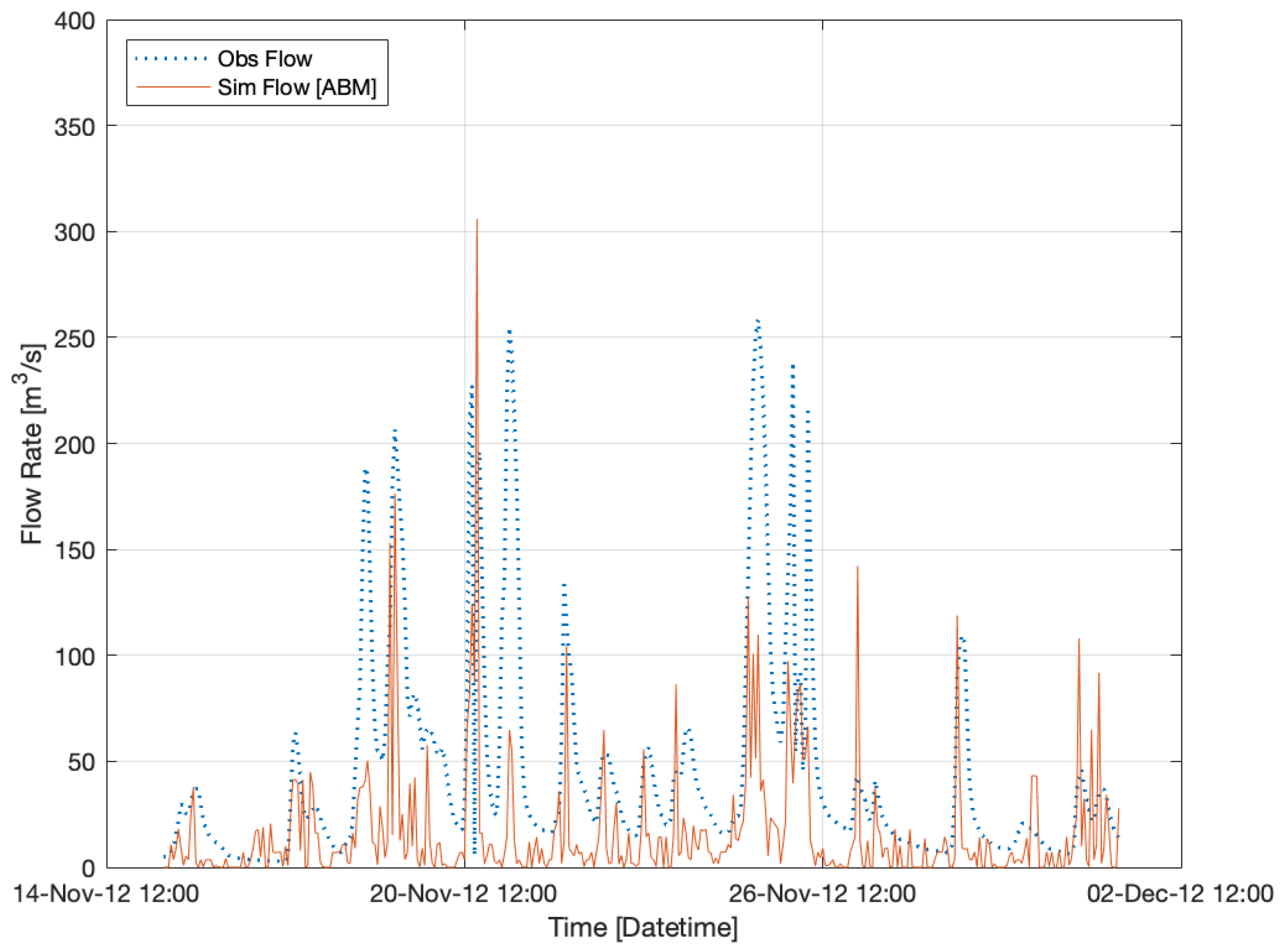
5.2.2. ABM: Validation, Comparing Single Storm-Based Simulation

The ABM streamflow simulation model was validated using data from other chosen storm periods described in Section 5.2. This is technically called the validation phase because new data are provided to the generated model, and its performance can be assessed to establish its overall goodness. Figure 21 shows the four measured storm periods, and the ABM-simulated hydrograph outputs, statistical measurements, and performance metrics are presented in

Table 9. Validation process. Measures of the statistics for the (ABM) flow hydrographs, both observed and simulated.

Validation Scenario	Cor. Coef. [r]	Coef. of Det. [R2]	RMSE [m3/s]	Percent. Error in Qpk [%]	Obs. Qpk [m3/s]	ABM Sim. Qpk [m3/s]
December 2012	0.86	0.74	25.1	51.7	266.4	404.0
December 2014	0.79	0.62	41.7	88.7	335.5	633.3
May 2015	0.76	0.58	20.1	28.1	257.1	329.3
November 2015	0.90	0.82	23.0	80.0	264.3	475.7

.

Four validation storms were selected and used in this strategy. The results from the third example, which simulated the storm of May 2015, were good, with a simulated peak discharge at the H3 station of roughly 329.3 m³/s; according to the observed peak streamflow (266.4 m³/s), it reflected an error of the spread between the two discharges of 20.1 m³/s and 28.1%, respectively. The simulation accuracy was only 58%, and the correlation coefficient (r = 0.76) was the smallest. Aside from the Q_pk% for the November 2015 verification storm, all examples showed that the errors were significantly lower than the calibration values.

In conclusion, the feasibility tests demonstrated that the ABM model hydrograph closely resembled the pattern of every single event validation storm episode hydrograph that was simulated. This indicates a high degree of agreement regarding the effectiveness of the ABM for simulating hydrologic flows in a tropical watershed over time. As a practical implementation option for HEC-HMS or other popular hydrologic models, this testing approach has also demonstrated that further model supplemental modification may enhance the correlation coefficient and gain a significant decrease in errors. This presumption is based on the commonly accepted notion that a respectable correlation factor should not be lower than 70%. Nevertheless, although this could represent the ideal scenario for each correlation research carried out on a particular dataset, it could fall short for many reasons, as Goodwin and Leech Goodwin and Leech [110] highlighted in the following six explanations of why a correlation strength might be undermined:

• Data with a high degree of variability
• Distinctive data distribution shape
• Lack of linearity
• Exceptions
• The sample’s features are distinct
• F-measures

6. Discussion

Based on the results collected, it can be said that streamflow simulation, calibration, and validation underscore a comprehensive effort to employ agent-based modeling (ABM) for hydrological modeling, specifically for simulating streamflow in each catchment area with a few to no displayed ground stations, which also could have severe data impairments. Initial simulations commenced with a warm-up phase utilizing observed data from a November 2012 storm event to configure the initial parameters of the model. This phase highlighted discrepancies between the observed and simulated flow hydrographs, indicating challenges in accurately capturing the peak flow magnitudes and the overall shape of the hydrograph. Despite attempts to calibrate the model using this initial dataset, the results exhibited significant deviations in peak discharge errors and a low correlation coefficient. This suggests that the model cannot accurately replicate the observed hydrological behavior under the tested conditions.

Subsequent calibration efforts involved a more nuanced approach, diverging from traditional hydrological models like HEC-HMS by leveraging the flexibility of ABM in the GAMA platform to conduct batch experiments for parameter adjustment. These experiments were tailored to enhance the model’s sensitivity to initial conditions and input variability, improving the alignment between the simulated and observed hydrographs. Four calibration scenarios were meticulously designed to refine the model inputs and parameters. This led to a noticeable improvement in model performance metrics, such as the correlation coefficient, root mean squared error (RMSE), and percentage error in peak runoff (Q_pk%). Despite the inherent challenges in calibrating agent-based models for complex hydrological processes, these efforts underscored the potential of ABM to achieve a reasonable degree of accuracy in simulating streamflow dynamics, especially with the application of advanced calibration techniques like multi-objective optimization and genetic algorithms [111,112,113,114].

Validation of the calibrated ABM model with data from additional storm events further attested to the model’s capability to simulate streamflow with acceptable accuracy. The validation phase demonstrated that the model could replicate the hydrological response of the catchment area for different storm events, as evidenced by the comparative analysis of the simulated and observed hydrographs across several validation storms. Although the model still exhibited some errors in the peak flow predictions, the overall performance metrics during the validation phase indicated a significant improvement from the initial warm-up simulations. This progression from calibration to validation illustrates the iterative nature of enhancing ABM models for hydrological simulations, highlighting the importance of rigorous calibration and validation processes in achieving reliable and accurate model outputs. Unfortunately, there was not at the time any relevant literature upon which to compare this approach; however, the journey from initial setup through calibration to validation reflects both the challenges and the potential of using ABM for detailed and dynamic hydrological modeling, suggesting that with continued refinement, ABM can serve as a viable tool for simulating streamflow in complex watershed systems.

It is worth mentioning that no previous study compared to this approach is available in the region that could be used for comparison purposes, suggesting that the uncertainty related to the model’s simulated discharge outputs against the limited records could be higher than that associated with the magnitude of the trends evaluated in this study. The streamflow, flooding, and water levels recorded at the H3 station experienced during the hydrologic conditions (monthly basis) for the five-year available record reflect the difficulties that the model could expect under approximately severe and prolonged hydrologic extremes, specifically in the absence of more representative hydrometric stations throughout the catchment.

7. Conclusions

Precise simulation and streamflow prediction are vital for reducing flood damage, highlighting the importance of streamflow modeling and forecasting in flood management efforts. Consequently, considerable research efforts have been dedicated to creating dependable models for prediction. These models need to consider a range of elements, including varying climates, streamflow characteristics, the availability and quality of data, and specific regional circumstances, with a particular focus on tropical regions. In this experimental approach, the feasibility of utilizing an agent-based model (ABM) for hydrologic flow simulation within a tropical river basin was investigated, and it has yielded promising results. The simulation outputs of the hydrograph patterns generated by the ABM have demonstrated high consistency with the observed hydrographs. This alignment has been further substantiated through rigorous calibration and validation processes, including applying robust statistical metrics.

The concurrence between the simulated and observed hydrographs, along with the statistical validation, underscores the potential of the ABM as a reliable tool for hydrologic flow simulation in the specific context of tropical river basins. The success achieved in this study paves the way for potential applications in water resource management and decision-making. Moreover, the adaptability of the ABM to accommodate refinements and enhancements presents an exciting avenue for future research and development.

Despite the model’s outcome, several implications and potential expansions remain that could be addressed, of which a few, if not all, are:

• Enhanced forecasting and control of flooding incidents.

Implication: The study’s implementation of an agent-based model (ABM) combined with data-driven modeling (DDM) and Artificial Intelligence (AI) provides a novel approach to simulating streamflow and accurately predicting flooding events.

Expansions: Future research could apply this framework to various river basins with different hydrologic characteristics to validate and refine the model’s predictive capabilities. Additionally, integrating new real-time data from advanced sensors could enhance the model’s responsiveness and accuracy in predicting imminent flood events.

2.

Improved comprehension of how water interacts with different processes.

Implications: By simulating streamflow interactions between river courses and their surroundings, the model offers a detailed spatial and temporal representation of hydrologic phenomena.

Expansions: Additional research could investigate the incorporation of more intricate environmental factors like soil moisture, changes in land use, and vegetation coverage. This exploration would help to better comprehend the overall ecological effects on streamflow and enhance watershed management practices.

3.

Use in Studies on the Impact of Climate Change

Implications: The model’s ability to simulate streamflow using historical precipitation, water level, and discharge data highlights its potential utility in climate change research.

Expansions: Researchers can expand the model to forecast future streamflow situations under various climate change projections. Climate models must be incorporated to evaluate the possible effects of shifting precipitation patterns and extreme weather events on river basins.

4.

Integration with Infrastructure Development and Urban Planning.

Implications: Precise modeling of river flow and maximum discharge has essential consequences for urban development, especially in creating robust infrastructure to endure floods.

As water management becomes increasingly critical in tropical regions, where unique climatic and hydrological dynamics often pose challenges, introducing a model like the ABM can significantly benefit experts and non-expert water practitioners. The accessibility and reliability of the ABM offer an asset for informed decision-making and sustainable water resource utilization.

In summary, this study’s outcomes highlight the potential of employing the agent-based model in hydrologic flow simulation within tropical river basins. With continued refinements, validations, and application-specific adaptations of fresh ground-based data, this model stands poised to emerge as a robust and indispensable tool for water practitioners, contributing to effective water management strategies and bolstering our capacity to address the complex hydrological challenges of tropical regions.

8. Future Work Plans

Future research directions related to model implementation with agent-based modeling for hydrologic flow simulation in a tropical river basin could include:

-

Incorporating more complex hydrological processes, such as adding meteorological variables, groundwater interactions, and riverbed processes, into the model to increase accuracy.

It is expanding the multi-agent system (MAS) framework to include more specialized agents with the BDI (Belief-Desire-Intention) model that can perform more specific tasks, such as Streamflow Forecasting and Flood-Awareness management.

-

Testing the model on different tropical river basins with varying characteristics, such as topography, geology, and vegetation cover, to assess its applicability and generalizability.

-

Incorporating uncertainty and sensitivity analysis to identify the most critical parameters and variables that affect the model’s outputs.

-

Creating an on-demand tracking system to continually update the model inputs and outputs for flooding projections and early notification systems may be helpful.

-

Collaborating with stakeholders, such as local communities, water managers, and policymakers, to integrate their perspectives and knowledge into the model’s development and implementation.

By addressing these research gaps, model implementation with agent-based modeling for hydrologic flow simulation in a tropical river basin can be further improved and applied to support sustainable water resource management in tropical regions.

References

1. FloodList Database. 2022. Available online: https://floodlist.com/ (accessed on 19 July 2022).
2. Eckstein, D.; Künzel, V.; Schäfer, L. Global Climate Risk Index 2021: Who Suffers Most from Extreme Weather Events; Germanwatch: Bonn, Germany, 2021; pp. 2000–2019. [Google Scholar]
3. Adikari, Y.; Yoshitani, J. Global Trends in Water-Related Disasters: An Insight for Policymakers; World Water Assessment Programme Side Publication Series, Insights; The United Nations, UNESCO: Paris, France; International Centre for Water Hazard and Risk Management (ICHARM): Tsukuba, Japan, 2009; pp. 1–24. [Google Scholar]
4. Wieriks, K.; Vlaanderen, N. Water-related disaster risk reduction: Time for preventive action! Position paper of the High Level Experts and Leaders Panel (HELP) on water and disasters. Water Policy 2015, 17 (Suppl. S1), 212–219. [Google Scholar] [CrossRef]
5. Devia, G.K.; Ganasri, B.P.; Dwarakish, G.S. A review on hydrological models. Aquat. Procedia 2015, 4, 1001–1007. [Google Scholar] [CrossRef]
6. Abdulkareem, J.; Pradhan, B.; Sulaiman, W.; Jamil, N. Review of studies on hydrological modelling in Malaysia. Model. Earth Syst. Environ. 2018, 4, 1577–1605. [Google Scholar] [CrossRef]
7. Jain, S.K.; Mani, P.; Jain, S.K.; Prakash, P.; Singh, V.P.; Tullos, D.; Kumar, S.; Agarwal, S.P.; Dimri, A.P. A Brief review of flood forecasting techniques and their applications. Int. J. River Basin Manag. 2018, 16, 329–344. [Google Scholar] [CrossRef]
8. Pandi, D.; Kothandaraman, S.; Kuppusamy, M. Hydrological models: A review. Int. J. Hydrol. Sci. Technol. 2021, 12, 223–242. [Google Scholar] [CrossRef]
9. Peel, M.C.; McMahon, T.A. Historical development of rainfall-runoff modeling. Wiley Interdiscip. Rev. Water 2020, 7, e1471. [Google Scholar] [CrossRef]
10. Sitterson, J.; Knightes, C.; Parmar, R.; Wolfe, K.; Avant, B.; Muche, M. An Overview of Rainfall-Runoff Model Types; U.S. Environmental Protection Agency: Washington, DC, USA, 2018. [Google Scholar]
11. Abudu, S.; Cui, C.-L.; King, J.P.; Abudukadeer, K. Comparison of performance of statistical models in forecasting monthly streamflow of Kizil River, China. Water Sci. Eng. 2010, 3, 269–281. [Google Scholar]
12. Kan, G.; He, X.; Li, J.; Ding, L.; Hong, Y.; Zhang, H.; Liang, K.; Zhang, M. Computer aided numerical methods for hydrological model calibration: An overview and recent development. Arch. Comput. Methods Eng. 2019, 26, 35–59. [Google Scholar] [CrossRef]
13. Veiga, V.B.; Hassan, Q.K.; He, J. Development of flow forecasting models in the Bow River at Calgary, Alberta, Canada. Water 2014, 7, 99–115. [Google Scholar] [CrossRef]
14. Wang, W. Stochasticity, Nonlinearity and Forecasting of Streamflow Processes; IOS Press: Amsterdam, The Netherlands, 2006. [Google Scholar]
15. Wang, W.; Vrijling, J.; Van Gelder, P.H.; Ma, J. Testing for nonlinearity of streamflow processes at different timescales. J. Hydrol. 2006, 322, 247–268. [Google Scholar] [CrossRef]
16. Yu, X.; Zhang, X.; Qin, H. A data-driven model based on Fourier transform and support vector regression for monthly reservoir inflow forecasting. J. Hydro-Environ. Res. 2018, 18, 12–24. [Google Scholar] [CrossRef]
17. Ji, J.; Choi, C.; Yu, M.; Yi, J. Comparison of a data-driven model and a physical model for flood forecasting. WIT Trans. Ecol. Environ. 2012, 159, 133–142. [Google Scholar]
18. Khatibi, R.; Ghorbani, M.A.; Kashani, M.H.; Kisi, O. Comparison of three artificial intelligence techniques for discharge routing. J. Hydrol. 2011, 403, 201–212. [Google Scholar] [CrossRef]
19. Shrestha, R.R.; Nestmann, F. Physically based and data-driven models and propagation of input uncertainties in river flood prediction. J. Hydrol. Eng. 2009, 14, 1309–1319. [Google Scholar] [CrossRef]
20. Borshchev, A.; Filippov, A. From system dynamics and discrete event to practical agent based modeling: Reasons, techniques, tools. In Proceedings of the 22nd International Conference of the System Dynamics Society, Oxford, England, 25–29 July 2004; Citeseer: Princeton, NJ, USA, 2004. [Google Scholar]
21. Chan, S. Complex adaptive systems. In ESD.83 Research Seminar in Engineering Systems; MIT: Cambridge, MA, USA, 2001. [Google Scholar]
22. Heath, B.L. The History, Philosophy, and Practice of Agent-Based Modeling and the Development of the Conceptual Model for Simulation Diagram. Ph.D. Thesis, Wright State University, Dayton, OH, USA, 2010. [Google Scholar]
23. Mckie, D. Complexity—The Emerging Science at the Edge of Order and Chaos—Waldrop, M.M. Media Cult. Soc. 1994, 16, 693–698. [Google Scholar] [CrossRef]
24. Agre, P.; Rosenschein, S.J. Computational Theories of Interaction and Agency; Mit Press: Cambridge, MA, USA, 1996. [Google Scholar]
25. Steinbacher, M.; Raddant, M.; Karimi, F.; Camacho Cuena, E.; Alfarano, S.; Iori, G.; Lux, T. Advances in the agent-based modeling of economic and social behavior. SN Bus. Econ. 2021, 1, 99. [Google Scholar] [CrossRef] [PubMed]
26. Axtell, R.L.; Farmer, J.D. Agent-based modeling in economics and finance: Past, present, and future. J. Econ. Lit. 2022, 60, 1–101. [Google Scholar]
27. Niazi, M.; Hussain, A. Agent-based computing from multi-agent systems to agent-based models: A visual survey. Scientometrics 2011, 89, 479–499. [Google Scholar] [CrossRef]
28. Macal, C.M.; North, M.J. Tutorial on agent-based modeling and simulation part 2: How to model with agents. In Proceedings of the 2006 Winter Simulation Conference, Monterey, CA, USA, 3–6 December 2006; Volume 1–5, pp. 73–83. [Google Scholar]
29. Macal, C.M. Tutorial on Agent-Based Modeling and Simulation: Abm Design for the Zombie Apocalypse. In Proceedings of the 2018 Winter Simulation Conference (Wsc), Gothenburg, Sweden, 9–12 December 2018; pp. 207–221. [Google Scholar]
30. Macal, C.M.; North, M.J. Tutorial on agent-based modelling and simulation. J. Simul. 2010, 4, 151–162. [Google Scholar] [CrossRef]
31. Taylor, S.J.E.; Anagnostou, A.; Kiss, T.; Terstyanszky, G.; Kacsuk, P.; Fantini, N. A Tutorial on Cloud Computing for Agent-Based Modeling & Simulation with Repast. In Proceedings of the 2014 Winter Simulation Conference (Wsc), Savannah, GA, USA, 7–10 December 2014; pp. 192–206. [Google Scholar]
32. Macal, C.M.; North, M.J. Tutorial on agent-based modeling and simulation. In Proceedings of the Winter Simulation Conference, Orlando, FL, USA, 4 December 2005; IEEE: Piscataway, NJ, USA, 2005. [Google Scholar]
33. De Almeida Falbo, R. SABiO: Systematic Approach for Building Ontologies. In Proceedings of the Onto.Com/odise@Fois. 2014, Rio de Janeiro, Brazil, 21 September 2014. [Google Scholar]
34. De Nicola, A.; Missikoff, M.; Navigli, R. A software engineering approach to ontology building. Inf. Syst 2009, 34, 258–275. [Google Scholar] [CrossRef]
35. Uschold, M.; Gruninger, M. Ontologies: Principles, methods and applications. Knowl. Eng. Rev. 1996, 11, 93–136. [Google Scholar] [CrossRef]
36. Uschold, M.; King, M. Towards a Methodology for Building Ontologies; AIAI-TR 183; Artificial Intelligence Applications Institute, University of Edinburgh: Edinburgh, UK, 1995; 13p. [Google Scholar]
37. Guarino, N. Formal Ontology in Information Systems: Proceedings of the First International Conference (FOIS’98), June 6–8, Trento, Italy; Frontiers in Artificial Intelligence and Applications; IOS Press: Amsterdam, The Netherlands, 1998; 337p. [Google Scholar]
38. Noy, N.F.; McGuinness, D.L. Ontology Development 101: A Guide to Creating Your First Ontology. 2001. Available online: http://protege.stanford.edu/publications (accessed on 18 June 2024).
39. Shurville, S. Model driven architecture and ontology development. Interact. Learn. Environ. 2007, 15, 96–99. [Google Scholar]
40. Neches, R.; Fikes, R.; Finin, T.; Gruber, T.; Patil, R.; Senator, T.; Swartout, W.R. Enabling Technology for Knowledge Sharing. AI Mag. 1991, 12, 36–56. [Google Scholar]
41. Agresta, A.; Fattoruso, G.; Pollino, M.; Pasanisi, F.; Tebano, C.; De Vito, S.; Di Francia, G. An Ontology Framework for Flooding Forecasting. In Computational Science and Its Applications–ICCSA 2014: 14th International Conference, Guimarães, Portugal, June 30–July 3, 2014, Proceedings, Part IV; Springer International Publishing: Cham, Switzerland, 2014; Volume 8582, pp. 417–428. [Google Scholar]
42. Sermet, Y.; Demir, I. Towards an information centric flood ontology for information management and communication. Earth Sci Inf. 2019, 12, 541–551. [Google Scholar] [CrossRef]
43. Wang, C.; Chen, Z.Q.; Chen, N.C.; Wang, W. A Hydrological Sensor Web Ontology Based on the SSN Ontology: A Case Study for a Flood. Isprs Int. J. Geo-Inf. 2018, 7, 2. [Google Scholar] [CrossRef]
44. Nikraz, M.; Caire, G.; Bahri, P.A. A methodology for the analysis and design of multi-agent systems using JADE. Int. J. Comput. Syst. Sci. Eng. 2006, 21, 1–40. [Google Scholar]
45. Amouroux, E.; Chu, T.-Q.; Boucher, A.; Drogoul, A. GAMA: An environment for implementing and running spatially explicit multi-agent simulations. In Proceedings of the Pacific Rim International Conference on Multi-Agents, Bangkok, Thailand, 21–23 November 2007; Springer: Berlin/Heidelberg, Germany, 2007. [Google Scholar]
46. Taillandier, P.; Gaudou, B.; Grignard, A.; Huynh, Q.-N.; Marilleau, N.; Caillou, P.; Philippon, D.; Drogoul, A. Building, composing and experimenting complex spatial models with the GAMA platform. GeoInformatica 2019, 23, 299–322. [Google Scholar] [CrossRef]
47. Simmonds, J.; Gómez, J.A.; Ledezma, A. The role of agent-based modeling and multi-agent systems in flood-based hydrological problems: A brief review. J. Water Clim. Change 2020, 11, 1580–1602. [Google Scholar] [CrossRef]
48. Brouwers, L.; Boman, M. A computational agent model of flood management strategies. In Regional Development: Concepts, Methodologies, Tools, and Applications; IGI Global: Hershey, PA, USA, 2012; pp. 522–534. [Google Scholar]
49. Anantsuksomsri, S.; Tontisirin, N. Agent-based modeling and disaster management. J. Archit./Plan. Res. Stud. (JARS) 2013, 10, 1–14. [Google Scholar]
50. Coates, G.; Hawe, G.; Wright, N.; Ahilan, S. Agent-based modelling and inundation prediction to enable the identification of businesses affected by flooding. WIT Trans. Ecol. Environ. 2014, 184, 13–22. [Google Scholar]
51. Berglund, E.Z. Using agent-based modeling for water resources planning and management. J. Water Resour. Plan. Manag. 2015, 141, 04015025. [Google Scholar] [CrossRef]
52. Yang, L.E.; Scheffran, J.; Süsser, D.; Dawson, R.; Chen, Y.D. Assessment of flood losses with household responses: Agent-based simulation in an urban catchment area. Environ. Model. Assess. 2018, 23, 369–388. [Google Scholar] [CrossRef]
53. Condro, A.A.; Widagdo, I.B. Katara: Model hidrologi berbasis agen (agent-based modelling) untuk analisis banjir di das ciliwung. J. Meteorol. Klimatol. Dan Geofis. 2019, 4, 1–7. [Google Scholar] [CrossRef]
54. Shirvani, M.; Kesserwani, G.; Richmond, P. Agent-based simulator of dynamic flood-people interactions. J. Flood Risk Manag. 2019, 14, e12695. [Google Scholar] [CrossRef]
55. Huber, L.; Bahro, N.; Leitinger, G.; Tappeiner, U.; Strasser, U. Agent-Based Modelling of a Coupled Water Demand and Supply System at the Catchment Scale. Sustainability 2019, 11, 6178. [Google Scholar] [CrossRef]
56. Farias, G.P.; Leitzke, B.; Born, M.; Aguiar, M.S.d.; Adamatti, D.F. Water Resources Analysis: An Approach based on Agent-Based Modeling. RITA 2020, 27, 81–95. [Google Scholar] [CrossRef]
57. Strahler, A.N. Hypsometric (area-altitude) analysis of erosional topography. Geol. Soc. Am. Bull. 1952, 63, 1117–1142. [Google Scholar] [CrossRef]
58. MPSA. Environmental Impact Assessment Study; MPSA: Bloomington, IN, USA, 2010. [Google Scholar]
59. Mockus, V. National Engineering Handbook; US Soil Conservation Service: Washington, DC, USA, 1964; Volume 4. [Google Scholar]
60. Wieder, W.; Boehnert, J.; Bonan, G.; Langseth, M. Regridded Harmonized World Soil Database v1.2; ORNL DAAC: Oak Ridge, TN, USA, 2014. [Google Scholar]
61. Sene, K. Flood Warning. In Flash Floods; Springer: Berlin/Heidelberg, Germany, 2013; pp. 169–198. [Google Scholar]
62. Simmonds, J.; Gómez, J.A.; Ledezma, A. Data Preprocessing to Enhance Flow Forecasting in a Tropical River Basin. In Proceedings of the Engineering Applications of Neural Networks: 18th International Conference, EANN 2017, Athens, Greece, 25–27 August 2017; Springer: Berlin/Heidelberg, Germany, 2017. [Google Scholar]
63. Little, R.J.; Rubin, D.B. Statistical Analysis with Missing Data; John Wiley & Sons: Hoboken, NJ, USA, 2019; Volume 793. [Google Scholar]
64. Wilkinson, L. Statistical methods in psychology journals: Guidelines and explanations. Am. Psychol. 1999, 54, 594. [Google Scholar] [CrossRef]
65. Bodner, T.E. Missing data: Prevalence and reporting practices. Psychol. Rep. 2006, 99, 675–680. [Google Scholar] [CrossRef] [PubMed]
66. Peugh, J.L.; Enders, C.K. Missing data in educational research: A review of reporting practices and suggestions for improvement. Rev. Educ. Res. 2004, 74, 525–556. [Google Scholar] [CrossRef]
67. Rubin, D. Inference and missing data. Biometrika 1976, 63, 581–592. [Google Scholar] [CrossRef]
68. Gao, Y.; Merz, C.; Lischeid, G.; Schneider, M. A review on missing hydrological data processing. Environ. Earth Sci. 2018, 77, 47. [Google Scholar] [CrossRef]
69. Hamzah, F.B.; Hamzah, F.M.; Razali, S.M.; Samad, H. A comparison of multiple imputation methods for recovering missing data in hydrological studies. Civ. Eng. J. 2021, 7, 1608–1619. [Google Scholar] [CrossRef]
70. Hamzah, F.B.; Mohamad Hamzah, F.; Mohd Razali, S.F.; El-Shafie, A. Multiple imputations by chained equations for recovering missing daily streamflow observations: A case study of Langat River basin in Malaysia. Hydrol. Sci. J. 2022, 67, 137–149. [Google Scholar] [CrossRef]
71. Umar, N.; Gray, A. Comparing single and multiple imputation approaches for missing values in univariate and multivariate water level data. Water 2023, 15, 1519. [Google Scholar] [CrossRef]
72. Lopucki, R.; Kiersztyn, A.; Pitucha, G.; Kitowski, I. Handling missing data in ecological studies: Ignoring gaps in the dataset can distort the inference. Ecol. Model. 2022, 468, 109964. [Google Scholar] [CrossRef]
73. R Core Team. R: A Language and Environment for Statistical Computing; R Foundation for Statistical Computing: Vienna, Austria, 2020. [Google Scholar]
74. van Buuren, S.; Groothuis-Oudshoorn, K. Mice: Multivariate Imputation by Chained Equations in R. J. Stat. Softw. 2011, 45, 1–67. [Google Scholar] [CrossRef]
75. Jang, J.-H. An advanced method to apply multiple rainfall thresholds for urban flood warnings. Water 2015, 7, 6056–6078. [Google Scholar] [CrossRef]
76. Blanc, J.; Hall, J.; Roche, N.; Dawson, R.; Cesses, Y.; Burton, A.; Kilsby, C. Enhanced efficiency of pluvial flood risk estimation in urban areas using spatial–temporal rainfall simulations. J. Flood Risk Manag. 2012, 5, 143–152. [Google Scholar] [CrossRef]
77. Cheng, C.S.; Li, Q.; Li, G.; Auld, H. Climate change and heavy rainfall-related water damage insurance claims and losses in Ontario, Canada. J. Water Resour. Prot. 2012, 4, 49–62. [Google Scholar] [CrossRef]
78. Hurford, A.; Parker, D.; Priest, S.; Lumbroso, D. Validating the return period of rainfall thresholds used for E xtreme R ainfall A lerts by linking rainfall intensities with observed surface water flood events. J. Flood Risk Manag. 2012, 5, 134–142. [Google Scholar] [CrossRef]
79. Priest, S.J.; Parker, D.J.; Hurford, A.P.; Walker, J.; Evans, K. Assessing options for the development of surface water flood warning in England and Wales. J Environ. Manag. 2011, 92, 3038–3048. [Google Scholar] [CrossRef] [PubMed]
80. Słownik, W. International Meteorological Vocabulary, 1992; WMO/OMM/IMGW: Geneva, Switzerland, 1992; p. 182. [Google Scholar]
81. Lam, H.; Lam, C.Y.; Wass, S.; Dupuy, C.; Chavaux, F.; Kootval, H. Guidelines on Cross-Border Exchange of Warnings; WMO/OMM/IMGW: Geneva, Switzerland, 2003; p. 182. [Google Scholar]
82. Sofiati, I.; Nurlatifah, A. The prediction of rainfall events using WRF (weather research and forecasting) model with ensemble technique. In Proceedings of IOP Conference Series: Earth and Environmental Science; IOP Publishing: Bristol, UK, 2019. [Google Scholar]
83. Dunkerley, D. Rain event properties in nature and in rainfall simulation experiments: A comparative review with recommendations for increasingly systematic study and reporting. Hydrol. Process. Int. J. 2008, 22, 4415–4435. [Google Scholar] [CrossRef]
84. Dunkerley, D.L. How do the rain rates of sub-event intervals such as the maximum 5-and 15-min rates (I5 or I30) relate to the properties of the enclosing rainfall event? Hydrol. Process. 2010, 24, 2425–2439. [Google Scholar] [CrossRef]
85. Mendham, P.; Clarke, T. Macsim: A simulink enabled environment for multi-agent system simulation. IFAC Proc. Vol. 2005, 38, 325–329. [Google Scholar] [CrossRef]
86. Neitsch, S.L.; Arnold, J.G.; Kiniry, J.R.; Williams, J.R. Soil and Water Assessment Tool Theoretical Documentation Version 2009; Texas Water Resources Institute: College Station, TX, USA, 2011. [Google Scholar]
87. Shannon, C.E.; Weaver, W. The Mathematical Theory of Communication; University of Illinois Press: Champaign, IL, USA, 1949. [Google Scholar]
88. Crooks, A.; Castle, C.; Batty, M. Key challenges in agent-based modelling for geo-spatial simulation. Comput. Environ. Urban Syst. 2008, 32, 417–430. [Google Scholar] [CrossRef]
89. Crooks, A.T.; Heppenstall, A.J. Introduction to agent-based modelling. In Agent-Based Models of Geographical Systems; Springer: Berlin/Heidelberg, Germany, 2011; pp. 85–105. [Google Scholar]
90. Klügl, F. A validation methodology for agent-based simulations. In Proceedings of the 2008 ACM Symposium on Applied Computing, Fortaleza, Brazil, 16–20 March 2008. [Google Scholar]
91. Parry, H.R. Agent-based modeling, large-scale simulations. In Complex Social and Behavioral Systems: Game Theory and Agent-Based Models; Springer: Berlin/Heidelberg, Germany, 2020; pp. 913–926. [Google Scholar]
92. Taillandier, P.; Vo, D.-A.; Amouroux, E.; Drogoul, A. GAMA: A simulation platform that integrates geographical information data, agent-based modeling and multi-scale control. In Proceedings of the Principles and Practice of Multi-Agent Systems: 13th International Conference, PRIMA 2010, Kolkata, India, 12–15 November 2010; Revised Selected Papers 13. Springer: Berlin/Heidelberg, Germany, 2010. [Google Scholar]
93. Vo, D.-A.; Drogoul, A.; Zucker, J.-D. An operational meta-model for handling multiple scales in agent-based simulations. In Proceedings of the 2012 IEEE RIVF International Conference on Computing & Communication Technologies, Research, Innovation, and Vision for the Future, Ho Chi Minh City, Vietnam, 27 February–1 March 2012; IEEE: Piscataway, NJ, USA, 2012. [Google Scholar]
94. Khu, S.T.; Madsen, H. Multiobjective calibration with Pareto preference ordering: An application to rainfall-runoff model calibration. Water Resour. Res. 2005, 41. [Google Scholar] [CrossRef]
95. Ngo, T.A.; See, L. Calibration and validation of agent-based models of land cover change. In Agent-Based Models of Geographical Systems; Springer: Berlin/Heidelberg, Germany, 2011; pp. 181–197. [Google Scholar]
96. Rogers, A.; Von Tessin, P. Multi-objective calibration for agent-based models. In Proceedings of the 5th Workshop on Agent-Based Simulation, Lisbon, Portugal, 3–5 May 2004. [Google Scholar]
97. Canessa, E.; Chaigneau, S. Calibrating agent-based models using a genetic algorithm. Stud. Inform. Control 2015, 24, 79–90. [Google Scholar] [CrossRef]
98. Cockrell, C.; An, G. Genetic Algorithms for model refinement and rule discovery in a high-dimensional agent-based model of inflammation. bioRxiv 2019, 790394. [Google Scholar]
99. Espinosa, O.B. A genetic algorithm for the calibration of a micro-simulation model. arXiv 2012, arXiv:1201.3456. [Google Scholar]
100. Boes, J.; Migeon, F. Self-organizing multi-agent systems for the control of complex systems. J. Syst. Softw. 2017, 134, 12–28. [Google Scholar] [CrossRef]
101. Caillou, P. Automated multi-agent simulation generation and validation. In Proceedings of the Principles and Practice of Multi-Agent Systems: 13th International Conference, PRIMA 2010, Kolkata, India, 12–15 November 2010; Revised Selected Papers 13. Springer: Berlin/Heidelberg, Germany, 2010. [Google Scholar]
102. Lomuscio, A.; Qu, H.; Raimondi, F. MCMAS: An open-source model checker for the verification of multi-agent systems. Int. J. Softw. Tools Technol. Transf. 2017, 19, 9–30. [Google Scholar] [CrossRef]
103. Oliveros, M.M.; Nagel, K. Automatic calibration of agent-based public transit assignment path choice to count data. Transp. Res. Part C Emerg. Technol. 2016, 64, 58–71. [Google Scholar] [CrossRef]
104. Drchal, J.; Čertický, M.; Jakob, M. Data driven validation framework for multi-agent activity-based models. In Proceedings of the Multi-Agent Based Simulation XVI: International Workshop, MABS 2015, Istanbul, Turkey, 5 May 2015; Revised Selected Papers 16. Springer: Berlin/Heidelberg, Germany, 2015. [Google Scholar]
105. Liu, Z.; Rexachs, D.; Epelde, F.; Luque, E. A simulation and optimization based method for calibrating agent-based emergency department models under data scarcity. Comput. Ind. Eng. 2017, 103, 300–309. [Google Scholar] [CrossRef]
106. Duda, P.; Hummel, P.; Donigian, A., Jr.; Imhoff, J. BASINS/HSPF: Model use, calibration, and validation. Trans. ASABE 2012, 55, 1523–1547. [Google Scholar] [CrossRef]
107. Fonseca, A.; Ames, D.P.; Yang, P.; Botelho, C.; Boaventura, R.; Vilar, V. Watershed model parameter estimation and uncertainty in data-limited environments. Environ. Model. Softw. 2014, 51, 84–93. [Google Scholar] [CrossRef]
108. Doyle, W.H.; Miller, J.E. Calibration of a Distributed Routing Rainfall-Runoff Model at Four Urban Sites Near Miami, Florida; US Geological Survey, Water Resources Division, Gulf Coast Hydroscience: Reston, VA, USA, 1980; Volume 80. [Google Scholar]
109. Shade, P.J. Hydrology and Sediment Transport, Moanalua Valley; US Geological Survey: Oahu, HI, USA, 1984; Volume 84. [Google Scholar]
110. Goodwin, L.D.; Leech, N.L. Understanding correlation: Factors that affect the size of R. J. Exp. Educ. 2006, 74, 249–266. [Google Scholar] [CrossRef]
111. Gutierrez, J.C.T.; Adamatti, D.S.; Bravo, J.M. A new stopping criterion for multi-objective evolutionary algorithms: Application in the calibration of a hydrologic model. Comput. Geosci. 2019, 23, 1219–1235. [Google Scholar] [CrossRef]
112. Herman, M.R.; Hernandez-Suarez, J.S.; Nejadhashemi, A.P.; Kropp, I.; Sadeghi, A.M. Evaluation of multi-and many-objective optimization techniques to improve the performance of a hydrologic model using evapotranspiration remote-sensing data. J. Hydrol. Eng. 2020, 25, 04020006. [Google Scholar] [CrossRef]
113. He, Q.; Molkenthin, F. Improving the integrated hydrological simulation on a data-scarce catchment with multi-objective calibration. J. Hydroinformatics 2021, 23, 267–283. [Google Scholar] [CrossRef]
114. Althoff, D.; Rodrigues, L.N. Goodness-of-fit criteria for hydrological models: Model calibration and performance assessment. J. Hydrol. 2021, 600, 126674. [Google Scholar] [CrossRef]
Figure 2. Hydrometric sensors for the flow simulation ontology are depicted in a UML layout.
Information 15 00448 g002
Figure 3. Schematics (Left) and sequence chart (Right) describing the steps of the ABM framework for hydrologic flow simulation.
Information 15 00448 g003
Figure 4. Medio River sub-catchment in the upper Caimito River Basin.
Information 15 00448 g004
Figure 5. Historic hydrologic record for the Medio River station H3, displaying rainfall [mm], stage [m], and streamflow [m3/s]. The figure illustrates the variations in these parameters over time and highlights the data gaps in the series from 2012 to 2016. This comprehensive record provides insight into the hydrologic patterns and anomalies within the specified timeframe.
Information 15 00448 g005
Figure 6. Average monthly rainfall [mm] at Station H3 for the study area (2012–2016).
Information 15 00448 g006
Figure 7. Average monthly streamflow [m3/s] at Station H3 for the study area (2012–2016).
Information 15 00448 g007
Figure 8. Stripplot: Comparing the distribution of the observed (Blue) and imputed (Red) datasets using the PMM technique with ten imputations for three variables. Imputed data are in red, whereas observed data are in blue.
Information 15 00448 g008
Figure 9. Historic hydrologic record for the Medio River station H3, displaying rainfall [mm], water level [m], and flow [m3/s] over the period 2012–2016. The figure includes imputed data to fill in the gaps in the original series, providing a complete and continuous dataset for analysis. This comprehensive record allows for a better understanding and modeling of hydrologic patterns and trends during this period.
Information 15 00448 g009
Figure 10. Historic rating curve containing instances of the imputed data for Medio River hydrometric station H3 (2012–2016).
Information 15 00448 g010
Figure 11. Hourly lag autocorrelogram for the H3 Hydrometric Station.
Information 15 00448 g011
Figure 12. Relationship between rainfall (Orange bar) and streamflow (Blue dotted line) during a possible storm at the Medio River Station H3 (November and December 2012).
Information 15 00448 g012
Figure 13. Relationship between rainfall (Orange bar) and streamflow (Blue dotted line) during a possible storm at Medio River Sta. H3. (December 2014).
Information 15 00448 g013
Figure 14. Relationship between rainfall (Orange bar) and streamflow (Blue dotted line) during a possible storm at Medio River Sta. H3. (May and November 2015).
Information 15 00448 g014
Figure 15. The flooded Medio River Catchment is depicted on the GAMA platform interface.
Information 15 00448 g015
Figure 16. GIS data source representing the Medio River. (a) Sub-catchments, (b) River Network, and (c) combined Sub-catchments and River Network.
Information 15 00448 g016
Figure 17. GIS data source representing the Medio River. (a) Sub-catchments IDs, (b) Non-Flooded River Network, and (c) Flooded River Network.
Information 15 00448 g017
Figure 18. Schematic diagram of the proposed ABM for hydrologic flow simulation, illustrating the intersecting functional layers: ‘hydrometric sensor level’ (HSn), ‘environment domain level’ (EDA), and ‘global agent’ (AgentGlobal) level. The figure highlights the role of the global agent in controlling other agents and the intra- and inter-agent communication required at the start of the simulation.
Information 15 00448 g018
Figure 19. Comparison of the flow hydrograph for the flood in November 2012 between observations and the ABM simulation.
Information 15 00448 g019
Figure 20. Measured vs. ABM flow simulation output for the storm in November 2012 following the calibration process: Scenarios 1 through 4.
Information 15 00448 g020
Figure 21. Measured vs. ABM flow simulation output for the four selected validation storms.
Information 15 00448 g021