Efficient Algorithms for Range Mode Queries in the Big Data Era

Abstract

The mode is a fundamental descriptive statistic in data analysis, signifying the most frequent element within a dataset. The range mode query (RMQ) problem expands upon this concept by preprocessing an array A containing n natural numbers. This allows for the swift determination of the mode within any subarray A[a..b], thus optimizing the computation of the mode for a multitude of range queries. The efficacy of this process bears considerable importance in data analytics and retrieval across diverse platforms, including but not limited to online shopping experiences and financial auditing systems. This study is dedicated to exploring and benchmarking different algorithms and data structures designed to tackle the RMQ problem. The goal is to not only address the theoretical aspects of RMQ but also to provide practical solutions that can be applied in real-world scenarios, such as the optimization of an online shopping platform’s understanding of customer preferences, enhancing the efficiency and effectiveness of data retrieval in large datasets.

1. Introduction

In the range mode query problem (RMQ), an array A of n natural numbers is given with q intervals. For each given interval we want to count its dominant, i.e., the element that occurs most often in a given fragment. It is easy to propose a naive solution running in linear time with the length of the interval. First, an improvement over the naive algorithm was proposed in [1]. The authors showed a deterministic algorithm to solve the RMQ problem in time $\mathcal{O}\left(n^{e}logn\right)$ and initialization time $\mathcal{O}\left(n^{2-2e}\right)$ where $e\in (0,1/2]$.

In [2], the authors showed a conditional lower bound for the RMQ problem using reduction from Boolean matrix multiplication. Each algorithm that solves the RMQ problem has an initialization time $\Omega \left(n^{\omega /2}\right)$ or query time $\Omega \left(n^{\omega /2-1}\right)$, where $\omega$ is the exponent of the multiplication algorithm matrix. There is currently no known combinatorial algorithm for Boolean matrix multiplication that would work in time $\mathcal{O}\left(n^{3-ϵ}\right)$, which means that, with the current state of knowledge, we cannot solve the RMQ problem initialization time $\mathcal{O}\left(n^{3/2-ϵ}\right)$ and query time $\mathcal{O}\left(n^{1/2-ϵ}\right)$ using purely combinatorial techniques.

In the same paper, the authors proposed an algorithm of $\mathcal{O}\left(\sqrt{n}\right)$ query time and $\mathcal{O}\left(n\sqrt{n}\right)$ initialization time. Later they showed its improvement in the standard RAM model, with query time $\mathcal{O}\left(\sqrt{n/w}\right)$ and initialization time $\mathcal{O}\left(n\sqrt{nw}\right)$, where w is the length of the machine word. Both algorithms drain out linear memory.

The aim of this work is the description, implementation, and comparative analysis of the above-mentioned algorithms and structure data for the RMQ problem. In particular, we only deal with algorithms that consume linear memory. In Section 3, we present the naive algorithm in two variants and then, in Section 4, we show it as a simple offline algorithm based on a naive algorithm. Then, we move on to the presentation algorithms from the papers mentioned above, starting with algorithm [1] in Section 5. The next Sections are devoted to [2]; in Section 6 we show the data structure corresponding to the RMQ query in time $\mathcal{O}\left(\sqrt{n}\right)$ and in Section 7 we present its improvement working in the RAM model. Next, we show in Section 8 a simple data structure whose query time depends on the number of unique elements of array A. In Section 9, we show a data structure that is a combination of the structures described in Section 7 and Section 8. Finally, in Section 11, we present the results of the evaluation of our implementations of the above algorithms and data structures.

1.1. Preliminaries

1.1.1. Notation

Tables. By $A[1:n]$ we will denote an array of n elements indexed from 1, and by $A\left[k\right]$ the k-th element. Similarly, we will denote a consistent fragment of array A from the i-th to the j-th element inclusive by $A[i:j]$ for $i\le j$. Where $i>j, A[i:j]$ means an empty fragment. For the interval $A[i:j]$ the subscript i will be called the left end of the interval and j the right end of the interval.

Frequency. For array A, by $F_x^A(i,j)$, we denote the frequency of x in the interval $A[i:j]$; then, the number of elements of $A\left[k\right]$ is equal to x for $k\in \{i,i+1,\dots ,j\}$. Moreover, we define $F^A(i,j)={max}_{k\in \left\{A\right[i],A[i+1],\dots ,A[j\left]\right\}}\left\{F_k^A(i,j)\right\}$. Instead of frequency, we will also use the name and number of occurrences interchangeably throughout the manuscript.

Dominance or mode. The element $A\left[k\right]$ of the array $A[1:n]$ is called dominant if $F_{A\left[k\right]}^A(1,n)=F^A(1,n)$, or in other words, $A\left[k\right]$ is the dominant (or mode) when it is the maximum element in terms of frequency in array A. Similarly, we define dominants on array intervals.

Data structure names. In case the data structure is not named in the paper, we refer to it through the initials of the authors of the work. In addition, some structures are parameterized with a number on which depends its memory or time complexity. For example, the structure CDLMW(s) is parameterized with a number s.

From now on, we will continue to use the name A to denote the input table for the algorithms and data structures. In addition, we denote by $\Delta$ the number of unique elements in array A.

1.1.2. Related Work

The range mode query problem was initially presented in [1]. They provided a useful observation and gave a solution with fast queries, achieving linear space and $\mathcal{O}(\sqrt{n}logn)$ query time. Afterwards, based on that useful observation, a number of efficient query solutions using linear space are proposed by researchers. The first solution achieving $\mathcal{O}\left(n\right)$ space and $\mathcal{O}\sqrt{n}$ query time is found in [3]. Later, work [2] improved the query time to $\mathcal{O}\left(\sqrt{{\displaystyle \frac{n}{logn}}}\right)$ with the knowledge from the world of succinct data structure. Meanwhile, strong evidence was given to indicate that a query time significantly below $\sqrt{n}$ cannot be reached by purely combinatorial techniques by reducing the multiplication of two $\sqrt{n}\times \sqrt{n}$ boolean matrices to the mode range query problem using linear space. The lower bound of the range mode query problem was proved later in the cell probe model, which states that, for any data structure that uses S memory cells of w-bit words, it takes $\Omega \left({\displaystyle \frac{logn}{log\left(\frac{S\times w}{n}\right)}}\right)$ query time to answer the range mode query problem. For linear space data structures in the RAM model, it corresponds to a lower bound of $\Omega \left({\displaystyle \frac{logn}{loglogn}}\right)$ query time, according to [3]. However, with current knowledge, there is no solution achieving the lower bound. Our main focus so far has been on linear space solutions to the static range mode query problem under the RAM model. Refer to

Table 1. Upper bounds of static and dynamic range mode query existing solutions.

Reference	Query Time	Update Time	Space	Type
[4]	$\mathcal{O}\left(n^{2/3}\right)$	$\mathcal{O}\left(n^{2/3}\right)$	$\mathcal{O}\left(n\right)$	Dynamic
[2]	$\mathcal{O}\left(n^{3/4}lglgn\right)$	$\mathcal{O}\left(n^{3/4}lglgn\right)$	$\mathcal{O}\left(n\right)$	Dynamic
[2]	$\mathcal{O}\left(n^{2/3}{\displaystyle \frac{lgn}{lglgn}}\right)$	$\mathcal{O}\left(n^{2/3}{\displaystyle \frac{lgn}{lglgn}}\right)$	$\mathcal{O}\left(n^{4/3}\right)$	Dynamic
[2]	$\mathcal{O}\left(\sqrt{{\displaystyle \frac{n}{lgn}}}\right)$	−	$\mathcal{O}\left(n\right)$	−
[3]	$\mathcal{O}\left(n^t\right)$	−	$\mathcal{O}\left(n^{2-2t}\right)$	$0<t\le {\displaystyle \frac{1}{2}}$
[3]	$\mathcal{O}(\Delta )$	−	$\mathcal{O}\left(n\right)$	−
[3]	$\mathcal{O}\left(m\right)$	−	$\mathcal{O}\left(n\right)$	−
[3]	$\mathcal{O}\left(\right|j-i\left|\right)$	−	$\mathcal{O}\left(1\right)$	−
[5]	$\mathcal{O}\left(1\right)$	−	$\mathcal{O}\left(n^2{\displaystyle \frac{lglgn}{{(lgn)}^2}}\right)$	−
[5]	$\mathcal{O}\left(n^t\right)$	−	$\mathcal{O}\left(n^{2-2t}\right)$	$0\le t<{\displaystyle \frac{1}{2}}$
[5]	$\mathcal{O}\left(1\right)$	−	$\mathcal{O}\left({\displaystyle \frac{n^2}{lgn}}\right)$	−
[5]	$\mathcal{O}\left(n^{t}lgn\right)$	−	$\mathcal{O}\left(n^{2-2t}\right)$	−
[1]	$\mathcal{O}\left(1\right)$	−	$\mathcal{O}\left(n^2{\displaystyle \frac{lglgn}{lgn}}\right)$	$0<t\le {\displaystyle \frac{1}{2}}$

for information about the current solutions found so far.

1.1.3. Rank Space Reduction

Let $D\left(x\right)$ denote the set of elements of the array $A[1:n]$ in the interval $A[1:x]$. We define the array $B[1:n]$ as rank space reduction, or table A reduction for short, when there is some bijection $f:D\left(n\right)\to$$\{1,2,\dots ,|D\left(n\right)\left|\right\}$ such that $B\left[i\right]=f\left(A\right[i\left]\right)$ for any $i\in \{1,2,\dots ,n\}$. Working on a reduced board, some operations can be performed on it more efficiently than an unreduced array. This is why, in discussing most of the algorithms in this paper, we will assume that the table we are working on is in this form. When we do not require the table to be reduced, we will write about it explicitly. In practice, we cannot assume that the given array on the input is reduced, so we give a linear, randomized algorithm for converting the $A[1:n]$ array to its reduced form as shown in Algorithm 1.

Algorithm 1 Randomized rank-space-reduction algorithm

1: procedure RankSpaceReduction($A[1:n]$)   2:       Let $B[1:n]$ be an array of n elements   3:       uniq ← HashMap()   4:       for $k\leftarrow 1,\dots n$ do   5:             if uniq.contains($A\left[i\right]$) then   6:                  B← uniq.get($A\left[i\right]$)   7:             else   8:                  B← uniq.size() + 1   9:                  uniq.insert($A\left[i\right]$, uniq.size() + 1) 10:           end if 11:      end for 12:      return B, uniq 13: end procedure

We maintain two invariants at the end of the loop:

• uniq represents a selection from a set $D\left(k\right)$ to {1,2, …,|D(k)|}.
• $B[1:k]$ is the reduction of $A[1:k]$ produced by applying uniq bijections to each element.

Finally, we return a reduced array B and a unique hashmap which, after reversing the keys with the values, will allow the input array A to be recreated.

1.2. Applications of Range Mode Query in Various Fields

1.2.1. Big Data Analysis

In the field of big data, RMQ’s role is invaluable in parsing through vast datasets to extract meaningful information. Big data often involves analyzing complex and large arrays $A[1:n]$, where n can be in the magnitude of millions or billions. RMQ algorithms facilitate the extraction of the most frequently occurring data points within specified intervals $A[i:j]$. This functionality is critical in various aspects of big data analysis [6], from market research and consumer behavior analysis to social media trend analysis and beyond.

For instance, in market research, RMQ can help identify the most popular product in a certain timeframe by analyzing sales data. In social media analysis, RMQ can be used to pinpoint trending topics or hashtags within certain time intervals. The frequency function $F_x^A(i,j)$ becomes a powerful tool in these scenarios, helping analysts to quickly determine the dominant element in the dataset. The ability of RMQ algorithms to handle large datasets efficiently makes them a go-to solution in the big data field, where data volume and the need for rapid processing are always pressing concerns.

1.2.2. Audit and Compliance

The application of the range mode query (RMQ) problem in audit and compliance is particularly profound due to its ability to efficiently handle large sets of transactional data, represented by an array $A[1:n]$. In the field of auditing, particularly financial auditing, RMQ serves as a powerful tool for identifying discrepancies and patterns that could indicate fraudulent activities or non-compliance with regulations.

Consider a scenario where a chief audit executive is examining the financial transactions of a company over a fiscal year. Each transaction is an element in the array A, and the auditor is interested in intervals $A[i:j]$ representing specific timeframes or transaction types. Using RMQ, the auditor can quickly ascertain the dominant transaction within these intervals, denoted as $F^A(i,j)$. This capability is crucial for detecting unusual patterns, such as a high frequency of certain transactions that might suggest embezzlement or money laundering.

Moreover, the advancements in RMQ algorithms, particularly those with time complexities like $\mathcal{O}\left(n\sqrt{nw}\right)$, where w is the length of the machine word, enable auditors to process large datasets rapidly. This speed is essential in audit scenarios where time is of the essence, such as in quarterly or annual financial reviews, or in investigations triggered by regulatory concerns. The application of RMQ in auditing not only enhances the accuracy of financial reviews but also significantly increases the efficiency of the auditing process.

1.2.3. Economic Data Analysis

Economic data analysis greatly benefits from RMQ, particularly in the assessment of market trends and consumer behavior. Utilizing RMQ to analyze intervals within economic datasets, represented by $A[i:j]$, allows economists to identify dominant economic indicators or trends. This capability is invaluable in forecasting and policy formulation, where understanding the frequency and occurrence ($F_x^A(i,j)$) of certain economic behaviors can lead to more informed decisions.

1.2.4. Healthcare

In medical research, RMQ can be employed to analyze patient data arrays $A[1:n]$, where each element represents a specific medical condition or symptom. By determining the dominant condition within different patient cohorts (intervals $A[i:j]$), healthcare professionals can identify prevalent health issues and tailor treatment plans accordingly. This application is especially relevant in epidemiological studies where understanding the frequency of symptoms can aid in disease control and prevention.

1.2.5. Retail and Marketing

Retailers can use RMQ to analyze customer purchase patterns over time. By identifying the most frequently bought items in different time intervals $A[i:j]$, retailers can optimize their inventory and tailor their marketing strategies to customer preferences. This insight is crucial for enhancing customer satisfaction and driving sales.

1.2.6. Technology and AI

In the realm of technology and artificial intelligence, RMQ finds its application in pattern recognition and user behavior analysis. Machine learning algorithms can incorporate RMQ to analyze data arrays $A[1:n]$, where each element represents a user action or preference, to identify the most common behaviors or preferences within specific timeframes. This application is instrumental in personalizing user experiences and improving interaction with technology.

2. Background and Related Work

2.1. Role of Big Data Analytics in Internal Audit

The role of big data analytics in modern internal audit practices has become increasingly crucial, and range mode queries play a significant part within this framework.

Big data analytics has emerged as a fundamental component of internal audit due to the growing volume and complexity of data within organizations. It involves the systematic analysis of vast datasets to extract meaningful insights, detect patterns, and identify anomalies [7]. This approach enables auditors to move beyond traditional audit methods and make data-driven decisions, enhancing audit effectiveness and efficiency.

Range mode queries, within the realm of big data analytics, offer a targeted approach to analyzing specific data ranges. They allow auditors to focus on subsets of data—defined by timeframes, numerical intervals, or other parameters—while simultaneously identifying the most frequent values or trends within these ranges [8]. This capability is particularly valuable in internal audits as it helps auditors uncover anomalies, irregularities, or outliers within targeted data sets.

In the context of internal audit, the application of range mode queries aligns with the broader objectives of data analytics by providing a method to sift through extensive datasets efficiently [9]. These queries assist auditors in identifying patterns or outliers that could signify potential risks, anomalies in financial or operational data, compliance deviations, or instances of fraud.

Moreover, the integration of range mode queries into big data analytics practices in internal audits fosters a more comprehensive understanding of data trends and behaviors [10]. By examining specific data ranges, auditors can gain insights into changes over time, and variations across different segments of data, and identify critical areas requiring further examination.

The utilization of range mode queries also enhances the ability to perform continuous monitoring and real-time analysis [11]. Auditors can leverage these queries to monitor ongoing data streams or periodic reports, enabling the proactive identification of emerging issues or trends.

Overall, in the context of big data analytics in internal audit, range mode queries offer a focused and efficient means to delve into specific data ranges [12]. They contribute to the broader goals of data-driven decision making, risk identification, anomaly detection, and continuous monitoring within modern internal audit practices, thereby augmenting the effectiveness and value of internal audit processes within organizations [13].

2.2. Range Mode Queries in Identifying Anomalies for Internal Audit

Range mode queries serve as crucial instruments in pinpointing anomalies or irregularities within financial or operational data during internal audit processes. They function by analyzing data within specified ranges, such as timeframes or numerical intervals, and identifying the mode (most frequent value) within these parameters [14]. This approach helps auditors to detect unusual patterns or outliers that significantly differ from expected or standard behaviors.

Financial audits benefit significantly from range mode queries, particularly in analyzing transactional data [15]. These queries can delve into specific date ranges or transaction amounts, effectively flagging anomalies like unexpected spikes in transaction values or unusually frequent occurrences of specific amounts [16]. Such anomalies serve as focal points for further detailed investigation by auditors, aiding in uncovering potential financial irregularities or discrepancies.

Beyond financial aspects, range mode queries also extend their utility to operational audits. They can analyze operational data like production output or inventory levels within defined ranges [17]. Sudden fluctuations or patterns that diverge from historical norms can signal operational irregularities or potential issues, guiding auditors towards areas necessitating scrutiny or corrective action.

Moreover, range mode queries play a pivotal role in compliance assessments. Auditors employ these queries to evaluate compliance with regulations or internal policies [18]. For instance, scrutinizing employee expenses within specific ranges can unveil patterns indicating non-compliance or potential risk areas where policies might not have been consistently adhered to.

Detecting potential fraud is another significant application. Range mode queries can flag unusual data patterns or irregular activities, serving as red flags for potential fraudulent behavior [19]. By identifying transactions significantly deviating from established norms, auditors can focus their investigative efforts on potential fraud risks.

Furthermore, these queries contribute to enhancing audit efficiency. Their targeted approach allows auditors to concentrate efforts on specific areas of concern rather than sifting through entire datasets. This precision maximizes the allocation of resources to areas exhibiting potential anomalies or risks, thereby streamlining the audit process.

The integration of range mode queries into continuous monitoring practices facilitates proactive anomaly detection over time. This approach aids in ongoing improvements to internal control systems, enabling auditors to maintain vigilance and prompt responses to emerging irregularities, ultimately strengthening the overall internal audit function.

2.3. Utilizing Range Mode Queries for Risk Assessment

Range mode queries offer valuable insights into risk assessment and mitigation strategies within internal audit processes by identifying trends and outliers within specific data ranges.

Firstly, these queries enable auditors to assess risks by analyzing data subsets within defined ranges. By focusing on specific intervals or categories, auditors can discern trends, patterns, or anomalies that might indicate potential risks [20]. For instance, in financial risk assessment, analyzing transactional data within certain timeframes can reveal patterns of irregularities, such as a sudden surge in high-risk transactions or unexpected fluctuations in revenue streams [21].

Moreover, range mode queries aid in identifying outliers within data ranges. Outliers, which represent data points significantly different from the majority, can signify potential risks or exceptional circumstances requiring closer scrutiny [22]. For example, in operational risk assessment, analyzing production metrics within defined ranges might expose outliers indicating equipment malfunction or unexpected operational disruptions.

The application of range mode queries extends to compliance risk assessment as well. By examining compliance-related data within specific ranges, auditors can identify deviations from established norms or policies [23]. Anomalies detected through these queries serve as indicators of potential compliance risks, prompting auditors to delve deeper into areas that might pose regulatory compliance challenges.

Additionally, range mode queries contribute to the identification of emerging risks. By continuously monitoring and analyzing data within defined ranges over time, auditors can spot evolving trends or patterns that might signal new risks [24]. This proactive approach enables auditors to anticipate and address potential risks before they escalate into significant issues. These queries aid in prioritizing risk areas [25]. By highlighting trends or outliers within specific data ranges, auditors can allocate resources more effectively, focusing attention on areas demonstrating higher risk potential. This targeted approach enhances the efficiency of risk mitigation efforts within the internal audit process.

Range mode queries serve as powerful tools in risk assessment by enabling auditors to delve into specific data ranges, and identify trends, outliers, and anomalies that signify potential risks. Their application spans various domains within internal audits, assisting auditors in proactively addressing risks and enhancing the overall risk management strategies of an organization.

2.4. Big Data and Range Mode Queries

Big data and range mode queries are interconnected within the realm of data analysis and are utilized to extract valuable insights from large and complex datasets.

Big data refers to the vast volumes of structured and unstructured data generated at high velocity from various sources. This influx of data presents both opportunities and challenges for organizations [26]. The sheer volume and variety of data make it challenging to extract meaningful insights using traditional analysis methods.

Range mode queries come into play as a valuable tool within big data analytics. They offer a focused approach to analyzing specific subsets or ranges of data. In the context of big data, where datasets are often extensive and diverse, range mode queries enable analysts to narrow their focus [27]. These queries help in pinpointing specific timeframes, numerical intervals, or other defined ranges within the vast dataset.

The significance of range mode queries in big data analytics lies in their ability to identify the most frequent values or trends within these defined ranges. This capability assists in uncovering patterns, anomalies, or outliers that might not be immediately apparent when dealing with the entire dataset [28]. By concentrating on these specific data ranges, analysts can gain valuable insights into trends, variations, or irregularities that might have implications for decision making or problem solving.

Also, within the context of big data, range mode queries contribute to the efficiency of analysis. They allow analysts to focus their attention on the subsets of data that are most relevant to the objectives of their analysis [29]. This focused approach helps streamline the analytical process, reducing computational overhead and enabling quicker identification of critical insights.

Range mode queries serve as a valuable tool within the realm of big data analytics by providing a focused and targeted approach to analyze specific subsets or ranges of extensive datasets. They assist analysts in uncovering patterns, anomalies, or trends that might not be readily apparent when dealing with the entirety of big data, thereby enhancing the effectiveness and efficiency of data analysis processes.

2.5. RMQ Applications in the Big Data Era

RMQ is a fundamental problem in Computer Science and Data Structures. It entails identifying the value that occurs most often when counting through the specified range of elements in an array. Although RMQ has been primarily discussed in algorithmic contexts alone, it can be extended to big data scenarios as volume, velocity, and variety are characteristics of big data. RMQ is a universal operation in a data structure that finds usage in applications such as big data processing, analyzing genetic sequences, and optimizing database queries. It encompass preprocessing an array in a way that makes it possible for one to be able to quantify on certain queries like the minimum value contained in a certain range of elements within the array. Compared to the traditional definition emphasizing the extraction of the minimum value in a range, RMQ can be extended for other variants of range query, including range frequency, range sum, etc. RMQ can be effectively applied to the fields of big data management, Automated Machine Learning, economics, and tree data structures [30,31,32,33,34,35].

2.6. Various Big Data Use Cases of RMQ

• Finding the Minimum Value in a Range

• Definition: Given an array A of n elements, preprocess A so that, for any given range $[i,j]$, the minimum value $min\left(A\right[i],A[i+1],\dots ,A[j\left]\right)$ can be found efficiently.
• Example: In stock price analysis, one might want to quickly determine the minimum stock price over a certain period.
• Mathematical Expression:

  $$\mathrm{RMQ}(i,j)=\underset{i\le k\le j}{min}A\left[k\right]$$

• Finding the Most Frequent Item in a Range

• Definition: Given an array A of n elements, preprocess A to efficiently find the most frequent item within any subarray $[i,j]$.
• Example: In analyzing user behavior on a website, one might need to determine which page was visited most frequently within a certain timeframe.
• Mathematical Expression:

  $$\mathrm{MFQ}(i,j)=arg\underset{v}{max}\left\{\mathrm{count}(v,A[i:j\left]\right)\right\}$$

• Finding the Sum of Elements in a Range

• Definition: Preprocess the array A to quickly compute the sum of elements within any given subarray $[i,j]$.
• Example: Summing up sales figures over a specified period.
• Mathematical Expression:

  $$\mathrm{RSQ}(i,j)=\sum _{k=i}^{j}A\left[k\right]$$

2.7. Detailed Use Case: Finding the Most Frequent Item in a Range

• Methodology

To efficiently find the most frequent item in a range, we can use a data structure called a Segment Tree or Sparse Table with additional frequency counting mechanisms.

• Preprocessing:
  • Construct a segment tree where each node stores the most frequent item and its count for the corresponding segment of the array.
  • Time Complexity: $O(nlogn)$ for building the segment tree.
• Querying:
  • For a given range $[i,j]$, traverse the segment tree to combine results from relevant segments to determine the most frequent item in that range.
  • Time Complexity: $O(logn)$ per query.

• Mathematical Explanation

Let A be the array and $F(i,j)$ be the function that returns the most frequent item in the subarray $A[i:j]$.

Using a segment tree,

• Define each node as $T\left[i\right]=(\mathrm{value},\mathrm{frequency})$, where “value” is the most frequent item in the segment represented by the node and “frequency” is its count.
• Merge function: When merging two nodes $T_l$ and $T_r$,

  $$T\left[i\right]=\left\{\begin{array}{cc}{T}_l\hfill & \mathrm{if}{T}_l.\mathrm{frequency}>T_r.\mathrm{frequency}\hfill \\ T_r\hfill & \mathrm{otherwise}\hfill \end{array}\right.$$

2.7.1. Data Preprocessing

Within the field of big data analysis, preprocessing is a fundamental first step that converts raw data into a format suitable for examination. This stage includes multiple processes such as data cleansing, conversion, and enrichment, all of which aim at ensuring the quality and validity of the information that would be required in further analysis steps [36]. RMQ algorithms are some of the most valuable tools in this phase given their ability to deal with large datasets [37]. They identify the least value within an array or dataset over a specified range of elements in an efficient way.

Making use of RMQ algorithms during preprocessing has several benefits.

• Firstly, this will take advantage of the RMQ algorithm to efficiently find out minimum values within specific ranges of data points. For example, when dealing with time series or geographical information datasets like temporal or spatial data, respectively, RMQ algorithms can find minimums and maximums very fast for predefined intervals [38]. This feature is useful when solving problems like trend analysis or anomaly detection where knowing differences within some ranges becomes necessary before making decisions about them [39].
• These also help in the cleaning of data and control of its quality during preprocessing. In certain ranges, these flags can be set by these algorithms to help check whether there are any issues with data quality [40]. For example, such robots may indicate faults or errors in measurements by the sensors as they assay readings from them.
• Additionally, RMQs participate in feature extraction and selection procedures [41]. Dimensionality reduction and focusing on the most significant attributes of data are common operations for many analytical tasks. As such, RMQs help find out the least values within some given feature ranges [42]. For example, this might include finding the darkest or brightest regions in an image that could be very important features for subsequent classification or segmentation stages in image processing.
• Normalization and scaling are supported in RMQ algorithms during preprocessing. These algorithms swiftly discover the minimum and maximum values across given ranges, which helps to normalize or scale data attributes [43]. This forms a basis for comparative purposes while maintaining the same range among the features and it is vital in normalizing the data before proceeding to any further analysis such as clustering or classification.
• In other words, RMQ algorithms enable the efficient identification of the minimum value within a specific data range thus making them essential tools for preprocessing big data analytics [44]. By ensuring that there is no compromise on either the quality or relevance of information manipulated by a given application, this step has contributed towards reducing the computational complexity associated with subsequent analysis tasks [45].

Ultimately, the utilization of RMQ algorithms improves the accuracy and insightfulness of analytical results leading to informed decision making in various domains.

2.7.2. Time Series Analysis

Time series analysis plays a role in big data applications across fields like finance, healthcare, manufacturing, and telecommunications [46]. It involves examining data collected at intervals over time to identify patterns, predict trends, and spot irregularities. RMQ (range mode query) algorithms are key, for handling queries and studying time series data in this context.

It is always very challenging to isolate trends and useful patterns in time series data. This helps analysts identify lower values within specified individual windows or intervals. By identifying the lowest values contained within fixed time spans, they enable them to unearth crucial fluctuations and trends in the information. For example, in financial market analysis, RMQ algorithms can identify the least valued stock price within a day or a week’s span where the market trend has been moving downward for any investment opportunity that may be present [47].

Moreover, RMQ algorithms are instrumental in detecting anomalies or outliers within time series data. Anomalies represent deviations from the expected behavior of the data and can indicate important events or irregularities [48]. By identifying minimum values within temporal intervals, RMQ algorithms assist in flagging unusual data points that fall below expected thresholds. For instance, in network traffic monitoring, RMQ algorithms can detect unusually low traffic volumes within hourly intervals, potentially signaling network disruptions or security incidents.

Furthermore, RMQ algorithms support the efficient computation of aggregate statistics over time series data. For instance, they can calculate the minimum value within sliding windows or rolling intervals, providing insights into the variability and stability of the data over time. This capability is essential for assessing the overall behavior of the time series and identifying periods of heightened or reduced activity. In manufacturing, for example, RMQ algorithms can compute the minimum production output within hourly shifts, helping managers optimize production schedules and resource allocation.

In summary, RMQ algorithms play a crucial role in time series analysis within the realm of big data applications. By enabling the efficient querying and analysis of time-varying datasets, these algorithms facilitate the detection of trends, patterns, and anomalies that are essential for informed decision making across various domains [49]. Whether in finance, healthcare, manufacturing, or telecommunications, RMQ algorithms provide valuable insights into the behavior and dynamics of time series data, ultimately driving improved outcomes and performance.

2.7.3. Data Compression and Summarization

Data compression and summarization are crucial techniques for managing the vast volumes of data generated in big data environments. These techniques aim to reduce storage requirements, minimize transmission times, and improve overall system efficiency [50]. RMQ (range mode query) algorithms offer a powerful approach to data compression and summarization by identifying representative minimum values within predefined ranges.

In the context of data compression, RMQ algorithms can be leveraged to identify minimum values within specific ranges of data points. By selecting representative minimum values and discarding redundant or less informative data, the overall dataset size can be significantly reduced [51]. For instance, in a time series dataset representing sensor readings, RMQ algorithms can identify minimum values within hourly intervals [52]. Storing only these representative minimum values rather than the entire dataset can lead to substantial storage savings, especially for datasets with high granularity and frequency.

Moreover, RMQ algorithms facilitate data summarization by providing insights into the overall distribution and characteristics of the data. By identifying minimum values within predefined ranges, these algorithms offer a concise summary of the dataset’s variability and trends [53]. For example, in financial market data, RMQ algorithms can identify minimum stock prices within daily intervals, summarizing the fluctuations and volatility of the market over time.

Furthermore the utilization of RMQ algorithms for data compression and summarization provides advantages that go beyond saving storage space. These techniques also enhance the efficiency of data transmission in environments with bandwidth. By decreasing the amount of data that must be sent, compression methods based on RMQ facilitate transfer speeds and reduce network delays [54]. This becomes crucial in scenarios involving distributed computing systems that require data exchange among nodes or across networks, with bandwidth capabilities.

Additionally, RMQ-based compression and summarization techniques can enhance data processing performance by reducing the computational overhead associated with analyzing large datasets. By working with compressed and summarized representations of the data, analytical tasks such as trend analysis, anomaly detection, and predictive modeling can be performed more efficiently [39]. This leads to faster insights and quicker decision making, essential qualities in today’s fast-paced business environments.

In summary, RMQ algorithms offer a valuable approach to data compression and summarization in big data environments. By identifying representative minimum values within predefined ranges, these algorithms enable significant storage savings, faster data transmission, and improved computational efficiency [55]. Whether in storage systems, network communications, or analytical workflows, leveraging RMQ-based compression techniques can help organizations better manage and derive value from their big data assets.

2.7.4. Parallel and Distributed Computing

In fact, parallel and distributed computing are essential paradigms, particularly for tackling the computational challenges of big data. RMQ (range mode query) algorithms are particularly well suited for this, as they can be effectively parallelized and distributed across multiple computing nodes [56]. By breaking the data into smaller segments and using parallel processing techniques, RMQ queries can be performed concurrently, thus providing significant performance and scalability improvements in large-scale distributed computing environments.

In parallel and distributed computing, RMQ algorithms can be parallelized by dividing the dataset into smaller segments or partitions, and distributing these segments across multiple computing nodes or processors [57]. What all of this means in practice, then, is that each node can process a particular subset of the data on its own with minimal node-to-node coordination and, as a result, RMQ queries can be executed across nodes in parallel. This approach leads to far faster query execution times than those you obtain with sequential processing [58]. RMQ queries can be executed simultaneously across multiple nodes. That, in turn, leads to substantially shorter query execution times than those that can be obtained with sequential processing (check out our programming team’s solution here).

In addition, distributed RMQ algorithms enable better and more efficient utilization of the available computational resources across multiple computing nodes via parallel processing techniques. By distributing the work across the nodes evenly, these algorithms can achieve a significantly greater degree of parallelism as well as scalability—even when dealing with very large datasets.

Moreover, RMQ algorithms can benefit from data partitioning strategies that optimize data locality and minimize data movement between computing nodes. By ensuring that related data elements are co-located within the same node or partition, these algorithms can reduce the communication overhead and latency associated with data transmission between nodes [59]. This approach is particularly important in distributed computing environments where network bandwidth and latency constraints may impact overall system performance.

Additionally, distributed RMQ algorithms can leverage fault tolerance mechanisms to ensure the reliability and robustness of computations in the face of node failures or network disruptions [60]. By replicating data and computation across multiple nodes, these algorithms can continue to operate seamlessly even in the presence of failures, thus enhancing system resilience and availability.

In scale distributed computing settings, parallel and distributed RMQ algorithms bring about enhancements in performance and scalability. These algorithms make use of processing methods, data partitioning strategies, and fault tolerance mechanisms to ensure the effective and scalable handling of big data [61]. They are tools for data-intensive applications whether used in cloud computing setups, distributed databases, or extensive analytics platforms. Parallel and distributed RMQ algorithms are vital for tackling the hurdles presented by big data.

3. Naive Algorithm

The first and at the same time the simplest algorithm we will describe is the naive algorithm in two variants. The first variant will not require the input table to be rank-space reduced, w opposite to the other.

3.1. Variant One

The naive algorithm does not require any preprocessing. The query algorithm is given in Algorithm 2. We use the unordered_map from the C++ standard library as the hashmap in this variant of the algorithm.

Algorithm 2 Naive Algorithm

1: procedure NaiveQuery($i,j$)   2:       count ← HashMap()   3:       mfreq ← 0   4:       mvalue ← 0   5:       for $k\leftarrow i,\dots j$ do   6:             freq ← 1   7:             if count.contains($A\left[k\right]$) then   8:                   $freq$← count.get($A\left[k\right]$) + 1   9:                   count$\left[A\right[k\left]\right]$$\leftarrow freq$ 10:                  if freq > mfreq then 11:                         mfreq ← freq 12:                         mvalue ←$A\left[k\right]$ 13:                  end if 14:            end if 15:      end for 16:      return mfreq, mvalue 17: end procedure

For a given query about the dominant in the interval $A[i:j]$ we will use a hashmap to count the frequency of its elements. We go over each element of $A\left[k\right]$ for $k\in \{i,i+1,\dots ,j\}$. When $A\left[k\right]$ is not in the hashmap, we add it to it with the value 1, otherwise we increase the value element in the hashmap by 1. During iteration, we store the maximum value contained in the hashmap and its corresponding key. After reviewing all elements, the hashmap will contain the frequencies of all values in the interval $A[i:j]$. So, the recorded maximum is the frequency of the dominant, and the corresponding key is the dominant on that interval.

3.1.1. Memory Complexity Analysis

For the query about the dominant in the interval $A[i:j]$ of elements in the hashmap, there is a maximum of $j-i+1$. On the other hand, there will never be more elements in a hashmap than $\Delta$. So, the total query algorithm consumes $\mathcal{O}(min(j-i,\Delta \left)\right)$ memory.

3.1.2. Time Complexity Analysis

During a single iteration of the loop, we use $\mathcal{O}\left(1\right)$ hashmap operations and $\mathcal{O}\left(1\right)$ arithmetic operations. The iteration of the loop is $j-i+1$. Assuming that all operations on the hashmap take amortized time $\mathcal{O}\left(1\right)$, the entire algorithm consumes $\mathcal{O}(j-i)$ time.

3.2. Variant Two

We note that in practice operations on a hashmap, although theoretically amortized, time constants are slower than array operations. Assuming the input array is rank-space reduced, we can replace the hashmap with an array of size $\Delta$.

Query algorithm: The query algorithm looks almost identical to the first variant. We replace the hashmap count by arrays of size $\Delta$. Also, at the very end of the algorithm before returning the dominant, we zero the elements of the count$\left[A\right[k\left]\right]$ array for $k\in \{i,i+1,\dots ,j\}$. The time complexity of the algorithm is the same as in the first variant.

Memory Complexity Analysis

In this variant, the count always takes $\mathcal{O}(\Delta )$ memory, so the whole data structure in total uses $\mathcal{O}(\Delta )$ memory.

4. Offline Algorithm

First, we introduce the MultiMode data structure, which will allow us to compute array A modes $A[k:l]$ from the mode $A[i:j]$ in time $\mathcal{O}\left(\right(|k-i|+|l-j|)logn)$. Next, we will show the algorithm (the given algorithm is sometimes referred to as “root-breaking” or “Mo’s algorithm”) using this data structure to handle a set of mode queries $Q=\left\{Q_1,Q_2,\dots ,Q_q\right\}$ in time $\mathcal{O}(n\sqrt{q}logn)$ where $q=\left|Q\right|$.

4.1. MultiMode Structure

We will show a MultiMode data structure that will hold some multiset M and support the following operations:

• INSERT(x)—insert x into the multiset M;
• REMOVE(x)—remove x from the multiset M;
• QUERY()—return the dominant and its frequency.

All operations run in $\mathcal{O}\left(logn\right)$ time; furthermore, we can build a MultiMode structure in $\mathcal{O}\left(1\right)$ time. The data structure will represent the multiset M by the hashmap count and binary tree search freqval. The count hashmap assigns a number to each unique element M occurrence. The binary freqval tree contains pairs ($count\left[v\right],v$) ordered by $count\left[v\right]$ for each key v hashmap $count$. Thanks to freqval, we will be able to query the hashmap key count with the maximum values, which will allow us to return the dominant in $\mathcal{O}\left(logn\right)$ time. The INSERT operation is given in Algorithm 3 while the REMOVE operation is given in Algorithm 4 and the QUERY operation is given in Algorithm 5.

Algorithm 3 Insert  Operation

1: procedure INSERT(x)   2:     freq ← 0   3:     if count.contains ($A\left[x\right]$ then   4:         freq ← count.get($A\left[x\right]$)   5:         freqval.remove((freq, $A\left[x\right]$))   6:     end if   7:     freq ← freq + 1   8:     freqval.insert ((freq, $A\left[x\right]$))   9:     count[$A\left[x\right]$] = freq 10: end procedure

Algorithm 4 Remove  Operation

1: procedure REMOVE(x) 2:     freq ← count.get($A\left[x\right]$) 3:     freqval.remove((freq, $A\left[x\right]$)) 4:     freq ← freq − 1 5:     if freq ≠ 0 then 6:         freqval.insert ((freq, $A\left[x\right]$)) 7:     end if 8:     count[$A\left[x\right]$] = freq 9: end procedure

Algorithm 5 Query  Operation

1: procedure QUERY(x) 2:     if freqval.size() = 0 then 3:         return (0, 0) 4:     end if 5:     return freqval.max() 6: end procedure

4.1.1. Insert Operation

When we add an element x to a multiset M, the number of its occurrences increases by 1, so we need to increment the x value in the count hashmap, which is on line 8 of the algorithm. After updating count we need to correct the $freqval$ task to match the changed hashmap count. If element x was found earlier than the multiset M, we need to remove the old pair in $freqval$ and insert a new one; we perform this accordingly in lines 5 and 7. In the second case, when x is a new unique element, M is enough to insert a new pair into $freqval$; we perform this in line 7.

4.1.2. Remove Operation

We assume that we want to remove an already existing value of x from the multiset M, so now we consider the case where x does not belong to M. The remove operation is analogous to the implementation of the insert operation.

4.1.3. Query Operation

If M is empty, we return a pair (0, 0), where the first element represents a number ascended and the second dominant. Otherwise, we return the largest element in the frequency.

4.1.4. Interval Transformation

Suppose we use a MultiMode structure to represent coherent array interval $A[i:j]$. We can replace the represented interval $A[i:j]$ with any other $A[k:l]$ by calling the insert and remove operations. We perform this in such a way that every step of the way the MultiMode structure represents a cohesive range of the array A. For example, when $j<l$, we call sequentially INSERT(x) for $x=i+1,i+2,\dots ,l$. We perform this in lines 2–4 of Algorithm 6. We handle the other three cases in a similar way.

Algorithm 6 Interval  transformation

1: procedure TRANSFORM($mm,i,j,k,l$)   2:     while $j<l$ do   3:         $mm.insert(j+1)$   4:         $j\leftarrow j+1$   5:     end while   6:     while $i<k$ do   7:         $mm.remove\left(i\right)$   8:         $i\leftarrow i+1$   9:     end while 10:     while $i>k$ do 11:         $mm.insert(i-1)$ 12:         $i\leftarrow i-i$ 13:     end while 14:     while $j>l$ do 15:         $mm.remove\left(j\right)$ 16:         $j\leftarrow j-1$ 17:     end while 18: end procedure

4.1.5. Alternative Implementation of MultiMode

Alternatively, a multiset M can be maintained by array $G[1:n]$ lists, where $G\left[i\right]$ stores in a list all unique elements with frequency i. The operation INSERT(x) can be performed in constant time by switching the element to the next list; analogically, remove operations can be handled. When implementing both operations, we keep the largest non-empty index list, which allows us to handle queries in constant time. Also, to find the corresponding item list x we scan for each unique element that has a list in an array or hashmap. We call this version MultiModeLIST and the original MultiModeBST.

4.1.6. Offline Queries

Suppose we want to answer a set of queries $Q=\left\{Q_1,Q_2,\dots ,Q_q\right\}$ about the dominants of array A. Let us denote $A[l_i:r_i]$ for range query for $Q_i$. Unfortunately, we cannot call transform in turn for queries $Q_1,Q_2,\dots ,Q_q$, because pessimistically the time complexity will be $\mathcal{O}\left(qnlogn\right)$. To remedy this, we will sort the queries in an appropriate way. We divide the query set Q into $s=\left[\sqrt{q}\right]$ separate parts. This is further shown in Algorithm 7.

Algorithm 7 Offline Query Algorithm

1: procedure Offline Query(Q)   2:     Let modes be a q-element array.   3:     Let U be a sequence of queries from Q in the order defined below.   4:     $mm\leftarrow MultiMode\left(\right)$   5:     $i\leftarrow 0$   6:     $j\leftarrow -1$   7:     for all $Q_i\in U$ do   8:         $transform(mm,i,j,l_i,r_i)$   9:         $i\leftarrow l_i$ 10:         $j\leftarrow r_i$ 11:         $modes\left[i\right]\leftarrow mm.query\left(\right)$ 12:     end for 13:     return modes 14: end procedure

Let $P_i$ denote the i-th part, for $i\in \{1,2,\dots ,s\}$. We define $P_i$ as $\left\{Q_k\mid ⌈l_{k}s/n⌉=i\right\}$. In other words, $P_i$ includes queries $Q_k$ whose left end $l_k$ lies in the interval $\left(\right(i-1)n/s,in/s]$. We mark by $p_k$ the number of the part to which the query $Q_k$$\left(Q_k\in P_{p_k}\right)$. Also, let U be the query sequence z of the set Q ordered lexicographically by pair $(p_i,r_i)$; equivalently, we can define the order $Q_i<Q_j⟺p_i<p_j\vee \left(p_i=p_j\wedge r_i<r_j\right)$.

4.1.7. Time Complexity Analysis

Variable initializations. We obtain the sequence U by ordering the set Q. We create this sequence using the merge sort algorithm, which will take $\mathcal{O}\left(qlogq\right)$ time.

Loop on line 7. Note that all queries belonging to the part $P_k$ form a coherent part for some k part of the sequence U. Therefore, we will divide the analysis into two cases. First, how long it takes to process queries in one part of $P_k$ and, second, how long it takes to go from one part to another.

First case. When the queries $Q_i$ and $Q_i+1$ belong to the same part of $P_k$, we know that their left ends are separated by a maximum of $n/s$ by definition of the part. So the transform function on line 8 will use at most $n/s$ insert or remove operations to move the left end. In total for the fixed parts of $P_k$, it will take $\mathcal{O}\left(\left|P_k\right|n/slogn\right)$ time to move the left ends. On the other hand, we know that the right ends of all queries in $P_k$ will be handled in non-decreasing order. So, in total, the function transform will invoke at most $\mathcal{O}\left(n\right)$ insert operations for a fixed $P_k$. So the time spent in case one we can estimate by $\mathcal{O}\left({\sum }_{k=1}^s\left[\left|P_k\right|n/slogn+nlogn\right]\right)=\mathcal{O}(qn/slogn+nslogn)=\mathcal{O}((q/s+s)nlogn)$.

Second case. In this case, we estimate that the transform function will not move the ends of the interval $A[i:j]$ by more than $2n$. Because queries from any fixed part of $P_k$ are a coherent fragment in the string U, $Q_i$ and $Q_i+1$ queries will be in different parts at most $s-1$ times. Totally, in the second case, we can estimate the time by $\mathcal{O}\left(snlogn\right)$.

Summary. Combining all the times above, we obtain a constraint $\mathcal{O}(qlogq+(q/s+s+1)nlogn)$. Substituting $s=\lceil \sqrt{q}\rceil$, we receive $\mathcal{O}(qlogq+n\sqrt{q}logn)\subset \mathcal{O}(n\sqrt{q}logn)$. The amortized time for one query takes $\mathcal{O}(n/\sqrt{q}logn)$ time. Using an alternative implementation MultiModeList, the factor of $logn$ disappears from the complexity time, so that the total time for this version is $\mathcal{O}(qlogq+n\sqrt{q})$ and the amortized time for a single query is $\mathcal{O}(logq+n/\sqrt{q})$.

4.1.8. Memory Complexity Analysis

The MultiModeBST structure occupies at most $\mathcal{O}(\Delta )$ of memory. A string of queries U occupies $\mathcal{O}\left(q\right)$ of memory, and its calculation requires the use of a sorting algorithm that also uses $\mathcal{O}\left(q\right)$ memory. We need the modes array to store the dominants which takes up $\mathcal{O}\left(q\right)$ of memory. The transform function uses a total of $\mathcal{O}\left(1\right)$ memory, including the insert and remove operations called. In total we use $\mathcal{O}\left(q\right)$ memory. Alternatively, the MultiModeLIST implementation maintains arrays of size n; using this version, in total, we use $\mathcal{O}(n+q)$ memory.

4.1.9. Implementation

As hashmaps, we used unordered_map from the standard c++ library and we used set as binary search trees, also from the c++ standard library. In addition, the numbers are rounded to the nearest power of two. This allows us to quickly calculate which part the query belongs to, which significantly speeds up the sorting of query set Q.

5. KMS(s) Data Structure

We will show the KMS(s) structure from work [1], parameterized after s, for a static array $A[1:n]$. This will support the following operations:

• COUNT(x,i,j)—returns $F_x^A(i,j)$ in $\mathcal{O}(logn)$ time.
• QUERY(i,j)—returns the dominant and its frequency in the interval $A[1:j]$ in time $\mathcal{O}(n/slogn)$.

5.1. KMS(s) Structure Construction

We create a $\Delta$ array $Q_x\left[0:F_x^A(1,n)-1\right]$ for each unique element $x\in \{1,2,\dots ,\Delta \}$. Table $Q_x$ at the i-th position holds the index (i + 1) of the occurrence of x in array A; in other words, $Q_x\left[i\right]=j⟺A\left[j\right]=x\wedge F_x^A(1,j)=i+1$. Moreover, we divide array A into s blocks, each but the last one of size $t=\lceil n/s\rceil$. The i-th block $B_i$ for $i=0,1,\dots ,s-1$ represents the interval $A[it+1,min(n,(i+1)t\left)\right]$. For each pair of blocks $B_i$, $B_j$, we store in a two-dimensional array $S[i,j]$ the dominant of a multiset $B_{i,j}=B_i\cup B_{i+1}\cup \cdots \cup B_j$. In addition, we store the two-dimensional array $S^{\prime }[i,j]$ which corresponds to the dominant frequencies $S[i,j]$ in the multiset $B_{i,j}$.

5.2. Count Operation

First, we will show how for any value $x\in \{1,2,\dots ,\Delta \}$ its frequency is calculated in the interval $A[i:j]$ in $\mathcal{O}\left(logn\right)$ time. Let $x_0<x_1<\cdots <x_{k-1}$ denote the indices of all occurrences of values of x in the interval $A[i:j]$. Since the $Q_x$ array is incremental, $x_0,\dots ,x_{k-1}$ answer a coherent fragment of the table $Q_x[l:l+k-1]$, where $Q_x[l+o]=x_o$ for $o\in \{0,1,\dots ,k-1\}$. We can easily find l using a binary search; this is the first value in the $Q_x$ array greater than or equal to i. Similarly, we are looking for the index m of the successor $x_k-1$ in the $Q_x$ table; it is the first value greater than j. In the case when $k=0$, we take $l=m=1$, and in the case when $x_k$ is the last occurrence of the value x in the table A we assume $m=F_x^A(1,n)$. Now, it is easy to see that $F_x^A(i,j)=m-l$. For example, consider the value 2 in the interval $A[8:14]$ in Figure 1. Number two occurs four times in this interval, on indices $x_0=9,x_1=11,x_2=13,x_3=14$, which correspond to the interval $Q_2[1:4]$. Using binary search we can quickly find the indices $l=1$ and $m=5$ corresponding to $x_0$ and the successor $x_3$ in table $Q_2$. From the indices $m,l$ we can calculate the frequency of element 2 in the interval $A[8:14]$: $F_2^A(8,14)=l-m=5-1=4$. This is further shown in Algorithm 8.

Algorithm 8 Operation  Count

1: procedure COUNT($x,i,j$) 2:     $m\leftarrow$ binary_search($Q_x,i$) 3:     $l\leftarrow$ binary_search($Q_x,j+1)$ 4: end procedure 5: return  $l-m$

5.3. Query Operation

Lemma 1. 

Let $A,B,C$ be multisets. If the dominant $A\cup B\cup C$ is neither in A nor in C then it is the dominant of the multiset B.

We will divide the query about the dominant in the interval $A[i:j]$ into two cases depending on the size of the interval. In the first case, when $j-i\le t$, we iterate linearly over the elements of the interval $A[i:j]$ (lines 4–13) and we count their frequency using the count operation. We return the element with the maximum frequency. In the second case, when $j-i>t$, the elements $A\left[i\right]$ and $A\left[j\right]$ are in different blocks. Let us mark by $b_i=\lfloor (i-1)/t\rfloor ,b_j=\lfloor (j-1)/t\rfloor$, respectively, the numbers of blocks to which elements $A\left[i\right]$ and $A\left[j\right]$ belong. We divide $A[i:j]$ into three parts, $A\left[i:\left(b_i+1\right)t\right],A\left[\left(b_i+1\right)t+1:b_{j}t\right]$, and $A\left[b_{j}t+1:j\right]$. Let us call the first and last parts with prefixes and suffixes. Then, we know from Lemma 1 that the dominant $A[i:j]$ is a dominant middle part or any of the elements of the prefix or suffix. We store the dominant middle part in $S\left[b_i+1,b_j-1\right]$ (lines 14–18) of Algorithm 9. The prefix and suffix are limited in size by t, so we support both fragments as in the first case (lines 20–27).

Algorithm 9 Query  Operation

1: procedure QUERY($i,j$)   2:     mfreq ← 0   3:     mmode ← 0   4:     if $j-i\le t$ then   5:         for k $\leftarrow i,i+1,\dots ,j$ do   6:            freq ← count($A\left[k\right],i,j)$   7:            if freq > mfreq then   8:                mfreq ← freq   9:                mmode ←$A\left[k\right]$ 10:            end if 11:         end for 12:     end if 13:     return mfreq, mmode 14:     $b_i\leftarrow [(i-1)/t]$ 15:     $b_j\leftarrow [(j-1)/t]$ 16:     if $b_i+1\le b_j-1$ then 17:         mfreq ←${\mathrm{S}}^{\prime }\left[b_i+1,b_j-1\right]$ 18:         mmode ←$\mathrm{S}\left[b_i+1,b_j-1\right]$ 19:     end if 20:     for k $ϵ$ prefix ∪ suffix do 21:         freq ← count($A\left[k\right],i,j)$ 22:         if freq > mfreq then 23:            mfreq ← freq 24:            mmode ←$A\left[k\right]$ 25:         end if 26:     end for 27:     return freq, mode 28: end procedure

5.4. Time Complexity Analysis

Construction. The $Q_i$ tables can be created in one scan of the A table, which consumes $\mathcal{O}\left(n\right)$ time. The i-th rows of arrays $S[i,\ast ],S^{\prime }[i,\ast ]$ we can create by linearly scanning array A. The row in arrays S and $S^{\prime }$ is s. In total, we need $\mathcal{O}\left(sn\right)$ time to construct the arrays S and $S^{\prime }$. Then, the structure construction of KMS(s) consumes $\mathcal{O}(n+sn)=\mathcal{O}\left(sn\right)$ time.

5.5. Operation Count

As mentioned earlier, the count operation takes $\mathcal{O}\left(logn\right)$ time because it uses two binary searches on $\mathcal{O}\left(n\right)$ data.

5.6. Operation Query

In the first case, when $j-i\le t$, the query operation performs the $\mathcal{O}\left(t\right)$ count operation; each takes $\mathcal{O}\left(logn\right)$ time, so the first case takes at most $\mathcal{O}\left(tlogn\right)$ time. In the second case, we perform the count operation by iterating over the prefix and suffix. The prefix and suffix are limited size by $\mathcal{O}\left(t\right)$. In total, the second case takes $\mathcal{O}\left(tlogn\right)$ time. Both cases are cumulative $\mathcal{O}(tlogn+tlogn)=\mathcal{O}(tlogn)$ time.

5.7. Memory Complexity Analysis

During construction, we create $\Delta$$Q_i$ arrays that together take up $\mathcal{O}\left(n\right)$ memory. Moreover, we create two two-dimensional arrays S and $S^{\prime }$ each of size $\mathcal{O}\left(s^2\right)$. The total data structure takes up $\mathcal{O}\left(n+s^2\right)$ memory.

5.8. Selection of Parameter s

Substituting $s=n^{1-e}$ for $e\in (0,1/2]$, we obtain a construction-time data structure $\mathcal{O}\left(n^{2-e}\right)$, which occupies $\mathcal{O}\left(n^{2-2e}\right)$ of memory. This allows calculation of the dominant in $\mathcal{O}\left(n^{e}logn\right)$ time. In particular, choosing $e=1/2$, we obtain linear memory and $\mathcal{O}(\sqrt{n}logn)$ query time.

6. CDLMW(s) Data Structure

The CDLMW(s) structure (Algorithm 1 from [2]) is a modification of the KMS(s) structure. The main change compared to the KMS(s) structure is how we handle the prefix and suffix during the query operation. Thanks to this change, we dispose of the logarithm during the query operation. By analogy with the structure of the KMS(s), we will partition array A into s blocks, each but the last one of size $t=\lceil n/s\rceil$. The i-th block $B_i$ for $i=0,1,\dots ,s-1$ represents the interval $A[it+1,min(n,(i+1)t\left)\right]$. The CDLMW(s) structure supports the following operations for a static array $A[1:n]$:

• COUNT($h,i,j)$—Calculates $F_{A\left[i\right]}^A(i,j)$ in time $\mathcal{O}\left(F_{A\left[i\right]}^A(i,j)-h\right)$. We assume that $1\le h\le F_{A\left[i\right]}^A(i,j)$.
• QUERY($i,j$)—Calculates the dominant and its frequency in $\mathcal{O}(n=s)$ time.

The h parameter of the count($h,i,j$) operation is a hint how many times at least the value $A\left[i\right]$ occurs in the interval $A[i:j]$.

6.1. CDLMW(s) Structure Construction

We construct the S, $S^{\prime }$, and $\Delta$$Q_x$ tables, which are described in the construction of the KMS data structure. In addition, we construct one additional array $R[1:n]$, which in the i-th position contains the value index $A\left[i\right]$ in table $Q_A{[}_i]$. Equivalently, we can define R to satisfy the following property: $Q_A{[}_i]\left[R{[}_i]\right]=i$.

6.2. Count Operation

Suppose we want to calculate $F_{A\left[i\right]}^A(i,j)$, with the additional knowledge that $A\left[i\right]$ occurs in the interval $A[i:j]$ at least h times. We know that all indices of occurrences $A\left[i\right]$ in the interval $A[i:j]$ form a coherent fragment in table $Q_A{[}_i]$. The R table allows us to find the beginning of this fragment in constant time. We could linearly scan this portion of $Q_A{[}_i]$ and find all occurrences of $A\left[i\right]$ in the interval $A[i:j]$. However, with hint h we can speed it up and skip the first h indices starting from the index $R\left[i\right]$ in the table $Q_A{[}_i]$. This is further shown in Algorithm 10.

Algorithm 10 Count  Operation

1: procedure COUNT($h,i,j$) 2:     $l\leftarrow R\left[i\right]$ 3:     $m\leftarrow R\left[i\right]+h$ 4:     while $m<size\left(Q_{A\left[i\right]}\right)\wedge Q_{A\left[i\right]}\left[m\right]\le j$ do 5:         $m\leftarrow m+1$ 6:     end while 7:     return $m-l$ 8: end procedure

6.3. Query Operation

Suppose we want to answer a query about the dominant in the interval $A[i:j]$. By analogy with the QUERY operation of the KMS structure, we denote $b_i=\lfloor (i-1)/t\rfloor ,b_j=\lfloor (j-1)/t\rfloor$, block numbers to which the elements $A\left[i\right]$, $A\left[j\right]$, respectively, belong. We divide the interval $A[i:j]$ into three parts, $A\left[i:min\left(j,\left(b_i+1\right)t\right)\right]$, $A\left[\left(b_i+1\right)t+1:b_{j}t\right]$, and $A\left[max\left(b_{j}t+1,\left(b_i+1\right)t+1\right):j\right]$. We call them prefix, middle, and suffix, respectively. The minima and maxima in the definition of the prefix and suffix guarantee that these ranges are disjoint in the case when $b_i=b_j$. When $b_i=b_j$, the middle and suffix are empty and when $b_i=b_j-1$ the middle is empty. If $b_i+1>b_j-1$, we take $S^{\prime }\left[b_i+1,b_j-1\right]=0$. This is further shown in Algorithm 11.

Algorithm 11 Query  Operation

1: procedure QUERY($i,j$)   2:     $b_i$$\leftarrow \left[\right(i-1)/t]$   3:     $b_j$$\leftarrow \left[\right(j-1)/t]$   4:     $mfreq\leftarrow S^{\prime }[b_i+1,b_j-1]$   5:     $mmode\leftarrow S[b_i+1,b_j-1]$   6:     for $\mathrm{k}\in$ prefix ∪ suffix do   7:         if $R\left[k\right]=0\vee Q_{A\left[i\right]}[R\left[k\right]-1]<i$ then   8:            if $k+m$ freq $<size\left(Q_{A\left[k\right]}\right)\wedge Q_{A\left[k\right]}[R\left[k\right]+m$ freq $]\le j$ then   9:                  $mfreq$$\leftarrow COUNT(mfreq+1,k,j)$ 10:                  $mmode\leftarrow A\left[k\right]$ 11:            end if 12:         end if 13:     end for 14:     return $mfreq,mmode$ 15: end procedure

To use the count operation efficiently, we will store the element m with the highest frequency middle and the prefix and suffix elements already reviewed in the loop on line 6. In the variables $mfreq$ and $mmode$ we store the frequency and value of this element accordingly. We call $A\left[k\right]$ a candidate prefix or suffix element if

• It lies within the range $A[i:j]$.
• It occurs at least $mfreq+1$ times in the interval $A[i:j]$.

If an element m is not dominant, then there must be an element $m^{\prime }$ that occurs more often than it in the interval $A[i:j]$. In particular, the first occurrence of $m^{\prime }$ in the interval $A[i:j]$ will be classified as a candidate. In this situation, when we encounter the first occurrence of $m^{\prime }$ in the loop on line 6, it will satisfy the candidate conditions and will pass the conditions in lines 7 and 8, in which we check (1) the condition and (2) being a candidate, respectively. Then, we replace element m with a newly found, more numerous, element $m^{\prime }$, whose frequency is calculated using the COUNT operation.

6.4. Computational Complexity Analysis

6.4.1. Construction

In addition to all the arrays of the KMS structure, we create one additional R array, which is easy to construct by linearly traversing the array $Q_x$ of total size n. So, we can construct the structure CDLMW(s) in $\mathcal{O}\left(ns\right)$ time.

6.4.2. Count Operation

We linearly scan the arrays $Q_A{[}_i]$ from position $R\left[i\right]+h$, and we know that $Q_{A\left[i\right]}\left[R\left[i\right]+\right.$$\left.F_{A\left[i\right]}^A(i,j)\right]>j$ so the loop on line 4 will not execute more than $\left.\left(R\left[i\right]+F_{A\left[i\right]}^A(i,j)\right)-(R\left[i\right]+h)\right)$$=F_{A\left[i\right]}^A(i,j)-h$ times. Each iteration takes $\mathcal{O}\left(1\right)$ time, so the count operation takes $\mathcal{O}\left(F_{A\left[i\right]}^A(i,j)-h\right)$ time.

6.4.3. Query Operation

We will analyze how much time we need in total for all count operations in line 9. Note that, if the loop of COUNT$(h,i,j)$ takes k steps, it returns $h+k$. We call this operation with $h=mfreq+1$, so for each iteration of the loop in the count operation we will increase $mfreq$ by 1. Let m be the dominant of the interval $A[i:j]$. Let us denote by $a,b,c$, respectively, the number of m entries in the prefix, middle, and suffix. The value of $mfreq$ is bounded by $a+b+c$, and its initial value is $S^{\prime }[b_i+1,b_j-1]$. Thanks to this, we know that the count operation will perform a maximum of $a+b+c-S^{\prime }[b_i+1,b_j-1]$ iterations. Moreover, we know that $b\le S^{\prime }[b_i+1,bj-1]$ and we can constrain $a,b$ by the block size t. Combining all this information we become constrained to all count operations in a single query: $\mathcal{O}\left(a+b+c-S^{\prime }\left[b_i+1,b_j-1\right]\right)\subset \mathcal{O}(a+c)\subset \mathcal{O}\left(t\right)=\mathcal{O}(n/s)$. Checking whether elements are candidates, we can limit by block size. Putting everything together, the query operation takes $\mathcal{O}(n/s)$ time.

6.4.4. Memory Complexity Analysis

We create one additional R array of size n compared to the KMS structure, so we need $\mathcal{O}(n+s^2)$ memory.

6.4.5. Count and Query Operations

We use constant memory during these operations.

7. CDLMW BP(s) Data Structure

This structure works assuming the standard RAM computation model with machine word $wϵ\Omega (logn)$ and requires that the dominant frequency is not greater than s. CDLMW BITPACKING structure, abbreviated CDLMW BP (Algorithm 2 from paper [2]) is a modification of the CDLMW structure, which changes the array representations of S to be more concise. In addition, we will not store the $S^{\prime }$ array. Thanks to these modifications, it has less memory consumption relative to the block size, which will allow us to choose more blocks $s=\sqrt{nw}$. Analogously to the KMS(s) structure, we will partition array A into s blocks, each except the last one of size $t=[n/s]$. The i-th block $B_i$ for $i=0,1,\dots ,s-1$ represents the interval $A[it+1,min(n,(i+1)t\left)\right]$. The CDLMW BP structure supports the following operations:

• BCOUNT($b_i,b_j)$—Calculates the dominant with the frequency of the interval
  $A\left[b_{i}t+1:min\left(n,\left(b_j+1\right)t\right)\right]$ in $\mathcal{O}(n/s)$ time when $b_i\le b_j<s$.
• COUNT($h,i,j)$—Calculates $F_{A\left[i\right]}^A(i,j)$ in time $\mathcal{O}\left(F_{A\left[i\right]}^A(i,j)-h\right)$.
  We assume that $1\le h\le F_{A\left[i\right]}^A(i,j)$.
• QUERY($i,j$)—Calculates the dominant and its frequency over time $\mathcal{O}(n/s)$.

The bcount($b_i,b_j$) operation computes exactly what was stored in the values of the arrays $S[b_i,b_j]$ and $S^{\prime }[b_i,b_j]$ in the KMS(s) structure.

7.1. Construction

We construct the R array which is described in the CDLMW data structure and construct the array $Q_x$ which is described in the KMS data structure. We create, for each $i\in \{0,1,\dots ,s-1\}$, a binary sequence $T\left[i\right]$, which corresponds to the row $S[i,\ast ]$ from the table in the KMS algorithm. For each $j\in \{i,i+1,\dots ,s-1\}$, we add at the end of the sequence $T\left[i\right]$ first $S[i,j]$ − $S[i,j-1]$ zeros, then one one. We accept $S[i,i-1]=0$. For example, row 2,3,5,5 is converted to the binary sequence 001010011.

7.2. RANK and SELECT Operations

For the binary sequence $B=\left(b_0,b_1,\dots ,b_{k-1}\right)$, and the number $b\in \{0,1\}$, we define operations $Ran{k}_b(B,i)$ = $\left|\left\{j\mid b_j=b\wedge j\in \{0,1,\dots ,i-1\}\right\}\right|$; in other words, $Ran{k}_b(B,i)$ is the number of elements of B equal to b in the interval $[0,i)$. We also define the operation $Selec{t}_b(B,i)$ = $min\left\{k\in \{1,2,\dots n\}\mid {rank}_b\left(k\right)=i\right\}$ which is the index of the i-th occurrence of b in sequence B, where $i>0$. This operation will allow us to efficiently extract information from the binary sequences contained in T. For example, knowing the position $p_j$ of the $j$-th one in the binary sequence $T\left[i\right]$, we can compute the frequency of the dominant $B_i\cup B_{i+1}\cdots \cup B_{i+j-1}$ by querying ${RANK}_0\left(T\left[i\right],p_j\right)$.

Of course, $p_j$ can be computed using $SELEC{T}_1(T\left[i\right],j)$. For the operation of the algorithm, it is crucial that these operations consume a maximum linear number of bits from the length of the string on which they operate. RANK and SELECT are the basis of succinct data structures; therefore, the following works are well studied [62,63,64]. For both operations there are sublinear memory consuming structures i allowing queries in constant time with linear construction time. However, we have decided to implement more practical [65,66] versions of these operations that consume more linear memory. We will describe the implementation of these operations in the following sections.

7.3. BCount Operation

Suppose we want to calculate the dominant $B_{b_i,b_j}=B_{b_i}\cup B_{b_i+1}\cup \cdots \cup B_{b_i}$ and its frequency. Let us define l by $l=b_{i}t+1,r=\left(b_j+1\right)t$, the left and right ends, respectively, of $B_{b_i,b_j}$. From the construction of $T\left[b_i\right]$, it is easy to note that the frequency of the dominant $B_{b_i,b_j}$ is the number of zeros between the beginning of the sequence $T\left[b_i\right]$ and its $(b_j-b_i+1)$. We perform this in lines 2–3. Next, note that the last zero before $(b_j-b_i+1)$-th was generated by some dominant $B_{b_i,b_j}$. We can find the position of this zero with one $Selec{t}_0$ query; we perform this in the fourth line. Knowing the position of the last zero generated by dominant $B_{b_i,b_j}$, it is easy to find which block this dominant is in with the $Selec{t}_1$ operation. We find the dominant $B_{b_i,b_j}$ by scanning the last block it contains; for each block element, we check that it occurs at least $F^A(l,r)$ times in $B_{b_i,b_j}$. This is further shown in Algorithm 12.

Algorithm 12 Bcount  Operation

1: procedure BCOUNT($b_i,b_j$)   2:     $po{s}_{b}j\leftarrow {select}_1\left(T\left[b_i\right],b_j-b_i+1\right)$   3:     $freq\leftarrow {rank}_0\left(T\left[b_i\right],{pos}_{b_j}\right)$   4:     ${\mathrm{pos}}_{\mathrm{last}}\leftarrow$ ${\mathrm{select}}_0\left(T\left[b_i\right]\right.$, freq )   5:     $b_{\mathrm{last}}\leftarrow {rank}_1\left(T\left[b_i\right]\right.$, $\left.{\mathrm{pos}}_{\mathrm{last}}\right)+b_i$   6:     first $\leftarrow t{b}_{\mathrm{last}}+1$   7:     last $\leftarrow min(n$, first $+t)$   8:         for $k\leftarrow$ first, …, last do   9:         if $R\left[k\right]-$ freq $+1\ge 0\wedge Q_{A\left[k\right]}[R\left[k\right]-$ freq $+1]\ge$ first then 10:         end if 11:     end for 12:     return $freq,A\left[k\right]$ 13: end procedure

7.4. Count and Query Operations

The COUNT operation remains unchanged from the CDLMW(s) structure; the only change in the operation query is the way to calculate the dominant $B_{bi+1,b_j-1}$. We use BCOUNT instead of accessing the tables S, $S^{\prime }$.

7.5. Time Complexity Analysis

7.5.1. Construction

The only analysis change to the CDLMW(s) structure is the construction of binary strings $T\left[i\right]$. We construct these sequences by scanning the array A about s times. The initialization of the rank and select operations is linear from the length of the binary sequence. Since we assumed that the frequency of the dominant is bounded by s, each binary string is a maximum of $2s$ in size. The construction T together with RANK and SELECT takes $\mathcal{O}\left(ns\right)$ time. In total, we need $\mathcal{O}\left(ns\right)$ time for constructions.

7.5.2. Bcount Operation

We use two RANK and SELECT operations, which take constant time. Moreover, linearly, we scan one block of size t. We need $\mathcal{O}\left(t\right)$ time in total.

7.5.3. Count Operation

Nothing has changed from the previous data structure. The COUNT operation requires $\mathcal{O}\left(F_{A\left[i\right]}^A(i,j)-h\right)$ time.

7.6. Query Operation

Relative to the previous data structure, the calculation of the freq variables and the model has increased to $\mathcal{O}\left(t\right)$ because we use the BCOUNT operation. However, this does not change the total time complexity of $\mathcal{O}\left(t\right)$.

7.7. Memory Complexity Analysis

7.7.1. Construction

Since we assumed the RAM model, we can pack the binary string T into machine words so we have s strings, each taking $\mathcal{O}(s/w)$ machine words. So, in a total of T strings, we need $\mathcal{O}(s^2/w)$ machine words, including support for the RANK and SELECT operations. Counting up to include the R and $\Delta$ arrays of the $Q_x$ arrays together consumes $\mathcal{O}(n+s^2/w)$ memory.

7.7.2. Bcount Operation

We use constant memory during this operation.

7.7.3. Count and Query Operations

The memory cost of these operations remains constant.

7.8. Selection of Parameters

Due to the reduced memory consumption, we can select a larger number of $s=\sqrt{nw}$ blocks which will give us a structure with a linear memory that allows us to calculate the dominants on any interval in time $\mathcal{O}\left(\sqrt{n/w}\right)$.

7.9. Implementation

In this section, we will be working with the binary sequence $B=\left(b_0,b_1,\dots ,b_{k-1}\right)$. For this, we would like quick responses to RANK and SELECT queries.

7.9.1. RANK

Construction. Let us assume that k is a multiple of 512. We divide sequence B into $k/512$ blocks $C_0,C_2,\dots ,C_{k/512-1}$, where the i-th block represents bits $B[512i:512(i+1)-1]$. In addition, we share each block $C_i$ into eight sub-blocks of form $D_{i,0},\dots ,D_{i,7}$, where the j-th sub-block represents the bits $B[512i+64j:512i+64(j+1)-1]$. For each $C_i$ block in the 64-bit number, we store $\overline{C_i}={RANK}_1(B,512i)$. Moreover, for each sub-block $D_i,j$ we store using 9 bits $\overline{D_{i,j}}={RANK}_1\left(C_i,64j\right)$. We can do so because each sub-block stores the ${RANK}_1$ of a string with a size of at most 512 bits, so the result will fit in 9 bits.

Query. Let us denote by $C_i,D_{i,j}$ the block and the sub-block to which $B[l-1$] belongs. We calculate the query RANK₁$(B,l)$ as follows: $\overline{C_i}+\overline{D_{i,j}}+{RANK}_1(B[512i+64j:i],l-512i-64j)$. The last RANK₁ is over the sequence with a maximum length of 64, which we can handle with the m_countbits_64 (https://software.intel.com/sites/landingpage/IntrinsicsGuide/#text=_mm_countbits_64, accessed on 1 July 2024) function at a time permanent. In practice, however, we use the builtin function builtin_popcountll (https://gcc.gnu.org/onlinedocs/gcc/Other-Builtins.html, accessed on 1 July 2024), which is supported by most major C++ compilers (GCC, Clang, MSVC). This generates the appropriate code machine based on the target platform.

Further Optimizations. $\overline{D_{i,0}}$ is always 0, so we do not need to store this value in memory. For each $C_i$ block, we store $\overline{C_i}$ and $\overline{D_{i,j}}$, where $j=1\dots 7. \overline{C_i}$ takes up to 64 bits, and $\overline{D_{i,j}}$ in total consumes 7 × 9 = 63 bits, so we can pack all $\overline{D_{i,j}}$ into one machine word. In addition, we note that, right after reading $\overline{C_i}$, we read $\overline{D_{i,j}}$, so we pack these two machine words next to each other in memory, to minimize the number of CPU cache misses. You can see what it looks like in the memory layout of this data in Figure 2. For every 512 bits, we use two 64-bit machine words. In summary, the memory overhead for the RANK₁ operation is 128 $[k/512]\approx 0.25k$ bits.

RANK₀. By using rank₀($B,i)$ we can handle by simple observation RANK₀($B,i$) = $i-$ RANK₁($B,i$).

7.9.2. SELECT

We implemented a slightly modified Algorithm 2 from [65]. Our modification consists in the use of two instructions, _pdep_u64 and _mm_tzcnt_64, available on Intel and AMD processors. These instructions will allow us to perform a SELECT₁ operation inside a machine word in constant time and constant memory. We denote by m the number of ones in B. For simplicity, let us assume that k is a multiple of w. We divide sequence B into $k/w$ blocks $C_0,C_1,\dots ,C_{k/w-1}$, where the i-th block represents bits $B\lceil wi:w(i+1)-1]$.

For the binary sequence B we define two derived binary sequences:

• The abbreviated sequence $S_B[0:k/w-1]$ of sequence B has a 1 in the i-th position when any bit of the block $C_i$ is not feeding. Otherwise, $S_B\left[i\right]$ = 0.
• The interrupting sequence $D_B[0:m-1]$ of B has a 1 in the i-th position when $(i+1)$-all 1 of B is the first one in the block containing it. Otherwise, $D_B\left[i\right]$ = 0.

Reducing the SELECT₁ in a single block. Our goal will be to reduce SELECT₁ ($B,i$) to a SELECT₁ operation inside a single block. To achieve this, we first show how to calculate SELECT₁ ($S_B,i$). The sequence $S_B$ is short, and its size is $n/w$. This allows us to remember the position of all ones. We need $log(n/w)$ bits to store one index. Indices to save are at most $n/w$. Using the assumption that w$ϵ$ $\Omega (logn)$, we can estimate the required memory by $\mathcal{O}(n/log(n)log(n/log\left(n\right)\left)\right)\subset \mathcal{O}(n/log(n)log(n\left)\right)=\mathcal{O}\left(n\right)$. Thanks to the SELECT₁ operation for the string $S_B$, we will be able to find the index of the k-th non-empty block in constant time. Moreover, we can find the number of non-empty blocks in which the i-th one is located using the RANK₁ ($D_B,i$) operation. Using these two operations, we can find the $s_i$ index of the block with the i-th one and p = RANK₁ ($B,s_{i}w$), the number of ones preceding the $C_{s}i$ block. Putting all this together, we obtain the formula: ${SELECT}_1(B,i)=s_{i}w+{SELECT}_1\left(C_{s_i},i-p\right)$.

We reduced ${SELECT}_1(B,i)$ to ${SELECT}_1$ in the $C_{s}i$ block. For example, we will find the fifth one in the sequence B in Figure 3. First, we find the number of the non-empty block in which the fifth one is located ${RANK}_1(D_B,5)$ = 3. Then, we calculate the index of block $s_i$ containing the fifth one, $s_i$ = ${SELECT}_1(S_B,3)$ = 3. Then, we count p the number of ones preceding the block $s_i$ as p = ${RANK}_1(B,s_{i}w)$ = ${RANK}_1(B,12)$ = 3. We use ${SELECT}_1(B,5)$ = $s_{i}w$ + ${SELECT}_1(C3,2)$ = 12 + 3 = 15. In the next paragraph, we show how to calculate ${SELECT}_1$ in block $C3$.

SELECT₁ in a single block. In this case, we use two processor instructions _pdep_u64 and _mm_tzcnt_64. Let $a[0:63]$ and $mks[0:63]$ be 64-bit numbers and $msk$ be a mask. Let l denote the number of non-zero bits $msk$ and $x_0,\dots ,x_{l-1}$ be indices of these bits. Then, _pdep_u64$(a,msk)$ will return a 64-bit number $K[0:63]$ defined as $K\left[xi\right]$ = $a\left[i\right]$ and $K\left[j\right]$ = 0 for $j\ne x_i$. Specifically, _pdep_u64$\left(2^{c-1},x\right)$ will return a number that has one non-zero bit in the c-th 1 position of x. The _mm_tzcnt_64 instruction allows us to find that position by counting the trailing zeros. For example, we will find the fifth one number a = 0100110011012. _pdep_u64$\left(2^{5-1}={00001}_2,{010011001101}_2\right)={000000000100}_2$. Now let us count the final zeros using _mm_tzcnt_64(${000000000100}_2$) = 9. The fifth one of a is in the ninth position.

Memory overhead. We need to perform rank operations on strings B and $D_B$, assuming to use the RANK9 structure we need ≈$2\times 0.25k=0.5k$ bits. The $D_B$ string itself takes pessimistically k bits. Also, we used ${SELECT}_1$ on the $S_B$ string, for which we stored all the positions of ones. Assuming $w\ge logk$, we use at most k bits. In total, we need at most $2.5k$ bits.

8. CDLMW SF Data Structure

We will present a data structure (Algorithm 3 from [2]) whose running time is sensitive to the number of unique elements $\Delta$. It supports one operation—QUERY$(i;j)$—returning the dominant $A[i:j]$, in time $\mathcal{O}(\Delta )$.

8.1. Construction

We divide array A into blocks of size $\Delta$, and let the last block be a smaller size. For each $i\in \left\{0,\dots ,⌈{\displaystyle \frac{n}{\Delta }}⌉\right\}$, we create the array $C_i[1:\Delta ]$, which contains a number in the j-th position of occurrences of the value j in the first i blocks. In other words, $C_i\left[j\right]$ is the number of occurrences of j in the interval $A[1:minn,i\Delta ]$. Figure 4 shows an example array and division into blocks of size $\Delta$ = 4.

Consider the query for the dominant in the interval $A[i:j]$. Let $b_j=[j/\Delta ]$ and $b_{i-1}$ = $\left[\right(i-1)/\Delta ]$ be the indices of the blocks to which the values $A\left[j\right]$ and $A[i-1]$ belong, respectively.

Let us note the frequency of all elements in the interval $A\left[b_{i-1}\Delta +1:b_j\Delta \right]$ can be computed by subtracting $C_{bi-1}$ from $C_{bj}$. Let us denote the difference between these two arrays by C. To obtain the frequency of all elements in the interval $A[i:j]$, missing values of $A[b_{i-1}\Delta :i]$ and redundant values of $A[j+1:b_j\Delta ]$ must be accounted for $\left(A\right[j+1:n]$ when $b_j$ is the last block). Let us call the missing elements a prefix and the excess elements a suffix. There are not many prefix and suffix elements, so we go through them one by one and update their frequency in table C.

8.2. Memory Complexity Analysis

We store $1+[n/\Delta ]$ arrays $C_i$, each of size $\Delta$. When calculating the dominant, we use a working table of size $\Delta$. In total, we use $(1+\lceil n/\Delta \rceil )\Delta +\Delta \in \mathcal{O}\left(n\right)$ memory.

8.3. Time Complexity Analysis

It takes $\mathcal{O}(\Delta )$ time to calculate the difference $C_{bj}-C_{bi-1}$. We can limit the size of the prefix and suffix from above by $\Delta -1$, so adding the prefix elements and subtracting the suffix elements together will take $\mathcal{O}(\Delta )$ time. Then, the query operations together take $\mathcal{O}(\Delta )$ time.

8.4. Implementation

Due to the fact that the $C_{bi-1}$ and $C_{bj}$ tables occupy a contiguous fragment of memory, we can easily vectorize them by calculating their difference. In our implementation, we use the vector instruction _mm512_sub_epi646 (https://software.intel.com/sites/landingpage/IntrinsicsGuide/#text=_mm512_sub_epi64, accessed on 1 July 2024) which allows you to subtract four 64-bit values at a time. This instruction is available on most new processors of Intel and AMD.

Depending on the size of the suffix, we may obtain better practical uptime by handling the suffix differently. Note that, instead of considering the entire block $b_j$ and then subtracting the suffix from it, we can equivalently ignore it and add the elements $A[(b_j-1)\Delta +1:j]$. In the case that the suffix $A[j+1:b_j\Delta ]$ is smaller than $[\Delta /2]$, we use the original processing; otherwise, we use the new one. Thanks to this pessimistically we will have to scan $[\Delta /2]$ instead of $\Delta -1$ elements. Analogous optimizations can be used for prefix scanning. Overall, pessimistically, we will have to scan $2[\Delta /2]$ elements instead of $2\Delta -2$.

9. CDLMW BP+SF Data Structure

This structure (the final algorithm from [2]) is a combination of the CDLMW BP and CDLMW SF structures. The structure of CDLMW BP assumes that the dominant cannot be large and CDLMW SF works fast when the number of unique items is limited. These methods perfectly complement each other, allowing you to bypass the limitations of both structures. The combined structure supports one operation—QUERY$(i;j)$—returning the dominant $A[i:j]$, in time $\mathcal{O}\left(\sqrt{n/w}\right)$.

9.1. Construction

We split the arrays $A[1:n]$ into two smaller arrays, $A_1[1:n^{\prime }]$ and $A_2[1:n-n^{\prime }]$. In table $A_1$, there are elements of the array A with a frequency of at most $\sqrt{nw}$, and the remaining elements of the $A_2$ table. The relative order in the tables $A_1$, $A_2$ is the same as in table A. We create $A_1,A_2$ by calculating the frequencies of all elements using a temporary array of size $\Delta$ and dividing array A with it. We construct the CDLMW BP($\sqrt{nw})$ structure for the $A_1$ table, and the CDLMW SF structure for the $A_2$ table. In addition, we will construct four arrays, $I_a[1:n],J_a[1:n]$, where $a\in \{1,2\}$. These allow us to convert the query about the dominant in the interval $A[i:j]$ into two sub-queries about the dominant of the arrays $A_a\left[I_a\left[i\right],J_a\left[j\right]\right]$. Formally, $I_a\left[i\right]$ is the index in the array $A_a$ of the first element A to the right of $A\left[i\right]$ that is in the array $A_a$. Analogously, we define $J_a\left[j\right]$ as the index of the array $A_a$ of the first element of the array A lying to the left of $A\left[j\right]$, which is in table $A_a$.

Query Operation

For the query about the dominant $A[i:j]$, we ask the substructures CDLMW BP and CDLMW SF about dominants in the intervals $A_1\left[I_1\left[i\right]:J_1\left[i\right]\right],A_2\left[I_2\left[i\right]:J_2\left[i\right]\right]$ and return the element with higher frequency. This is shown in detail in Algorithm 13.

Algorithm 13 Query  Operation

1: procedure SFQUERY($i,j$)   2:     Let $C[1:\Delta ]$ be a temporary array   3:     $b_{i-1}\leftarrow [(i-1)/\Delta ]$   4:     $b_j\leftarrow [j/\Delta ]$   5:     for $k\leftarrow 1,\dots ,\Delta$ do   6:         $C_k\left[k\right]\leftarrow C_{bj}\left[k\right]-C_{bi-1}\left[k\right]$   7:     end for   8:     prefix $\leftarrow min(n,b_{i-1}\Delta )$   9:     for $k\leftarrow i,\dots ,$prefix do 10:         $C\left[A\right[k\left]\right]\leftarrow C\left[A\right[k\left]\right]+1$ 11:         $suffix\leftarrow min(n,b_j\Delta )$ 12:     end for 13:     for $k\leftarrow j+1,\dots ,$suffix do 14:         $C\left[A\right[k\left]\right]\leftarrow C\left[A\right[k\left]\right]-1$ 15:     end for 16:     $mode\leftarrow argmaxC$ 17:     return $C\left[mode\right],mode$ 18: end procedure

9.2. Time Complexity Analysis

9.2.1. Construction

Tables $I_a,J_a$ can easily be constructed by going through array A once. Substructures need $\mathcal{O}\left(n\sqrt{nw}\right)$ and $\mathcal{O}\left(n\right)$ construction time. In total, we need $\mathcal{O}\left(n\sqrt{nw}\right)$ construction time.

9.2.2. Query Operation

We note that array $A_2$ has a maximum of $n/\sqrt{nw}=\sqrt{n/w}$ items. So, both substructures need $\mathcal{O}\left(\sqrt{n/w}\right)$ time to count the dominants, so the query operation runs in time $\mathcal{O}\left(\sqrt{n/w}\right)$.

9.3. Memory Complexity Analysis

9.3.1. Construction

Both structures consume linear memory, as $I_{*},J_{*}$ arrays do. So, we need the total available linear memory.

9.3.2. Query Operation

In this operation, we perform operations on structures where each consumes additional constant memory. So, we are using $\mathcal{O}\left(1\right)$ memory.

10. Proposed Methods

In this section, we propose an $\mathcal{O}\left(m\right)$ query time and $\mathcal{O}\left(n\right)$ space method using a linear-space data structure. The main idea is derived from [1].

Lemma 2. 

Let $A1$ and $A2$ be any multisets. If c is a mode of $A1\cup A2$ and $c\notin A1$, then c is a mode of $A2$.

How can we apply this lemma to the range mode query problem? Assume that the target range is divided into two sections, A1 and A2. The mode of the range $A1\cup A2$ is either the mode of the range $A2$ or one of the elements within the range of $A1$.

Following previous works, we partition an A array into $[s=n/m]$ blocks of size $t=m$. Then, the target range $[i,j]$ is partitioned into either of the two following scenarios:

• When i mod t = 0, we keep the original target range.
• Otherwise, it is separated into two parts which are the prefix $[i,[i/t]\times t-1]$ and the suffix $\left[\right[i/t\times t,j]$.

We precompute tables $Array1[0:s-1,1:m]$ and $Array2$ (which is the mode) as $[0:s-1,1:m]$ for each $b_i\in \{0,\cdots ,s-1\}$ and $b_j\in \{1,\cdots ,m\}$. $Array1\left[b_i\right]\left[b_j\right]$ stores the smallest index $x\le n$ such that the node of the range $[b_i\times m,x]$ has $b_j$ frequency at the most. If the frequency of the mode cannot reach $b_j$ then x is set to n. $Array2\left[b_i\right]\left[b_j\right]$ stores the corresponding mode.

To check whether each element in the prefix is a candidate mode, we use the same method introduced in [2]. Hence, besides the two tables $Array1$ and $Array2$, we also require another $\Delta +1$ array. For each $a\in \{1,$⋯, $\Delta \}$, let array $Q\left[a\right]$ store the set of indices b such that $A\left[b\right]=a$. Moreover, the last one array is $A^{\prime }[1:n]$, such that, for each b, let $A^{\prime }\left[b\right]$ store the index of b in an array $Q\left[A\right[b\left]\right]$.

Each of the data structures mentioned here uses $\mathcal{O}\left(n\right)$ space. The algorithm to construct $Array1$ and $Array2$ is as follows in Algorithm 14.

Algorithm 14 Precomputation of Array1 and Array2

1: procedure  PRECOMPUTATION   2:     Initialize $Array1[s\_num\_block][m\_freq+1]$   3:     Initialize $Array2[s\_num\_block][m\_freq+1]$   4:     for $s\leftarrow 0$ to $s\_num\_block$ -1 do   5:         Initialize the array $count\_item[\Delta ]$   6:         $array1\left[s\right]\left[1\right]\leftarrow t\_of\_block\times s$   7:         $array2\left[s\right]\left[1\right]\leftarrow original\_arr[t\_of\_block\times s]$   8:         $index\leftarrow 2$   9:         for $i\leftarrow (t\_of\_block\times s)$ to ($original\_arr.length-1)$ do 10:            $count\_item[original\_arr[i\left]\right]++$ 11:            if $count\_item[original\_arr[i]=index$ then 12:                $array1\left[s\right]\left[index\right]\leftarrow i$ 13:                $array2\left[s\right]\left[index\right]\leftarrow original\_arr\left[i\right]$ 14:                $index++$ 15:            end if 16:            for $j\leftarrow index$ to $m\_freq$ do 17:                $array1\left[s\right]\left[j\right]\leftarrow original\_arr.length$ 18:                $array2\left[s\right]\left[j\right]\leftarrow array2\left[s\right][j-1]$ 19:            end for 20:         end for 21:     end for 22: end procedure

From Algorithm 14, it can be seen that it requires $\mathcal{O}(s\times m)$ time to complete.

Query Algorithm

Suppose that the target range has been partitioned into two parts, the prefix $[i,b_j-1]$ and the suffix $[b_j,j]$. For the suffix part, we can find the predecessor of j in the subarray $Array1\left[[b_j/t]\right]$. Here, the predecessor means the leftmost maximum element in $Array1\left[[b_j/t]\right]$ which is not larger than j.

Let f denote the index of the predecessor in the array $Array1\left[[b_j/t]\right]$. Then, f represents the frequency of the mode in the suffix range and $Array2\left[[b_j/t]\right]\left[f\right]$ stores the corresponding mode. To find the predecessor, there are three ways. Linear scan requires $\mathcal{O}\left(m\right)$ time in the worst case, as there are m elements in the array $Array1\left[[b_j/t]\right]$. Considering that $Array1\left[[b_j/t]\right]$ is a monotonically increasing sequence, binary search can also be applied which requires $\mathcal{O}\left(logm\right)$ time.

If we use the advanced data structure, namely Van Emde Boas Tree, because of the type of the array $Array1\left[[b_j/t]\right]$, we will require $\mathcal{O}\left(loglogn\right)$ time as $\{1,\cdots ,n\}$. For simplicity reasons, we use the same linear scan method as in [2] in order to find the candidate mode in the prefix whose frequency in the range $[i,j]$ is larger than the frequency f of the mode in the suffix range. The query cost is bounded by $\mathcal{O}(t=m)$. Summing up using the prefix and suffix altogether, the overall cost to find the mode in a range $[i,j]$ is $\mathcal{O}\left(m\right)$.

11. Experimental Results

11.1. Test Data and Queries

We conducted performance tests of the construction time and query time of all implemented algorithms and data structures. In order to carry out the tests, we generated examples of arrays with sizes ranging from 1000 to 4,000,000 elements. We divided these tables into three categories depending on the number of unique elements $\Delta =64,\Delta =\sqrt{n}$, and $\Delta =n/64$.

For each array of size n, we generated n queries. Also, any query we represented as uniformly drawn two numbers $i,j\in \{1,2,\dots ,n\}$ that correspond to queries for the interval $A\left[min\right(i,j):max(i,j\left)\right]$. By such selection of queries to the data, each query has an expected length $1/3n$. The length of the interval is of particular importance for naive algorithms, in which the query time is directly dependent on it. In addition, for offline algorithms, we generated additional tests with a variable number of queries to examine what effect it has on the query time.

Table 2. Software and hardware components used for the experiments.

Operating system	Windows 11
Kernel version	22H2
Processor	Intel i9-10850k CPU @ $5.00\mathrm{GHz}$
Cache L1/L2/L3	$64\mathrm{KiB}$/$256\mathrm{KiB}$/$20\mathrm{MiB}$
Cache patency	5
Processor extensions used	AVX512VL, MBI2

presents the components utilized in the experiments.

11.2. Naive Algorithm

11.2.1. Initialization Time

The initialization time of the first variant (Figure 5 left-hand side) is practically zero; in our implementation we will remember the pointer to the table on which we will execute queries. On the other hand, during the variant second initialization (Figure 5 right-hand side), we create an array replacing the hashmap in the first variant. We could create it for every one together during the query, although the query time would increase from $\mathcal{O}(j-i)$ to $\mathcal{O}(max(\Delta ,j-i\left)\right)$. As seen in Figure 5, the initialization time does increase, although it is negligibly low compared to a single query.

11.2.2. Query Time

In our data, the expected length of a query depends linearly on the number of elements, so we predict that the query time of the naive algorithm will also be linear with the size. Exactly this behavior is observed in Figure 6. Moreover, we can see that the naive algorithm for a linear number of unique items works out about one and a half times slower compared to other categories of data. We suspect this is due to the greater number of elements in the hashmap. You can find the right value generates more CPU cache misses.

As we suspected, the second variant is definitely faster (about 6 × faster) in comparison to the first variant. Operations on a hashmap, although theoretically in constant time, in practice are a lot slower than array operations.

11.3. Offline Algorithm

11.3.1. Initialization Time

The initialization time of the offline algorithm in both variants is analogous to the second variant of the algorithm naive. In the first implementation, using binary trees, we create an array to replace the hashmap for counting elements and, in the second case, we additionally create arrays of lists. In both implementations, the initialization time is negligibly small compared to the query time.

11.3.2. Query Time

For a given array size, we generated a linear number of queries, so we predict running time $\mathcal{O}\left(\sqrt{n}logn\right)$ in BST and $\mathcal{O}\left(\sqrt{n}\right)$ in the list version for a single query. We note that the implementation using a list array is definitely better, and works 7–15 × faster as shown in Figure 7.

11.3.3. Query Time vs. Number of Queries

The offline algorithm is the only algorithm we describe whose running time depends on the number of queries. Therefore, in the interest of completeness, we conducted tests to check how the algorithm behaves offline depending on the number of requests. This is further shown in Figure 8. We performed experiments for n = 400,000.

11.4. CDLMW and CDLMW BP Data Structures

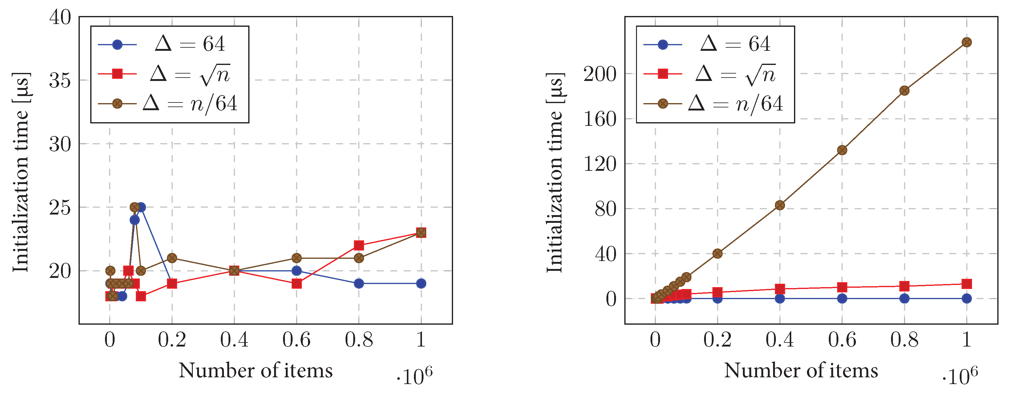
11.4.1. Initialization Time

We remind you that the initialization time of the CDLMW and CDLMW BP data structures is, respectively, $\mathcal{O}\left(n\sqrt{n}\right),\mathcal{O}\left(n\sqrt{nw}\right)$. In our implementation, the machine word $w=64$, so the BP version blocks are $\sqrt{w}=8$ times smaller. For this reason, we expect at least eight times slower structure creation time in the BP version. In practice, distributions $\Delta =16$ and $\Delta =\sqrt{n}$ are performing better; the BP structure works around 6.5 times slower. In the case of a large number of unique elements, the BP structure is eight times slower. We suspected that the additional initialization of rank and select in the BP version of the data structure may have a significant impact on construction time. After using profiler (https://perf.wiki.kernel.org/index.php/Tutorial, accessed on 1 July 2024), we found out that more than 90% of the time during initialization is taken by computing the mode for each pair of blocks. To confirm this, we decided to increase the number of blocks in the CDLMW algorithm to $\sqrt{nw}$. We obtained very close initialization times to the BP version. The results are shown in Figure 9.

11.4.2. Query Time

During the query in the BP version, we scan one block more, so we expect the query to be $8\times (2/3)=5, 33$ times faster than the basic version of the algorithm. In practice, however, this is not the case when the number of elements is small; we experience about three times acceleration. With the increase in the number of unique elements, we obtain about 4.75 times acceleration for data $\Delta =\sqrt{n}$ and $\Delta =n/64$ as shown in Figure 10.

11.5. CDLMW SF Data Structure

11.5.1. Initialization Time

The initialization time of the CDLMW SF data structure depends linearly on the table size. In Figure 11, we can observe that, in practice, the more unique elements, the longer the initialization time.

11.5.2. Query Time

We conducted query time tests for two versions of the CDLMW SF structure: with the optimizations described in Section 8.4, and without optimization. The test results can be seen in Figure 12 (left with optimization and right without). For data with a fixed number of unique elements, the query time in both versions is practically the same. For category $\Delta =\sqrt{n}$ and $\Delta =n/64$, the optimized version is about 1.25 times faster than the ordinary.

11.6. CDLMW BP+SF Data Structure

Initialization and Query Time

We remind you that the initialization time of the CDLMW BP + SF structure is $\mathcal{O}\left(n\sqrt{nw}\right)$. For data categories $\Delta =64$ and $\Delta =\sqrt{n}$, Figure 12 (left-hand side) reflects this; however, for type $\Delta =64$ at $n\ge {512}^2\approx 2.6\ast {10}^5$, there is a sudden drop in initialization time. The expected frequency of each element is greater than $\sqrt{nw}$ meaning that all elements are handled by the CDLMW SF substructure, which has a much faster, linear, initialization time as proven by Figure 13.

11.7. Assessment of $\Delta$ Size

In this section, we conduct experiments on an accounting dataset [67], particularly related to audits and transactions. The dataset contains more than 1800 observations related to audits on financial firms. We assess all methods under various $\Delta$ sizes. The results of the KMS and CDLMW data structures are given in Figure 14.

The results of the CDLMW BP and CDLMW SF are given in Figure 15. Lastly, we evaluate the CDLMW BP + SF method. The results are given in Figure 16.

12. Conclusions

In this section, we will try to answer the question of what algorithm/data structure should be used, to solve the RMQ problem as soon as possible. Naive algorithm: We recommend using the naive algorithm when the sum of the lengths of the intervals query does not exceed n. All the data structures described need at least a linear time per initialization; we can use this time to calculate the mode as well.

For the offline algorithm at the outset, we note that there is no point in using the BST variant; it is from 7 to 15 times slower than the LIST version. When the RMQ algorithm runs in $f\left(n\right)\ge logn$ time, then we use the offline algorithm when the number of queries $\left|Q\right|\ge C{(n/f\left(x\right))}^2$ for a properly selected constant C. For such a selection $\left|Q\right|$, the offline algorithm does not work slower than the algorithm. Especially for algorithms CDLMW SF and CDLMW BP + SF, we select the number of queries $128{(n/\Delta )}^2$ and $2{(n/\sqrt{n/w})}^2$ for which the offline LIST algorithm achieves similar query times.

As for the KMS data structure, we do not recommend using this structure; the CDLMW structure has practically identical initialization time and at the same time faster query operations.

CDLMW SF data structure: When there are no more than 45 unique elements $45\sqrt{n/w}$, we propose using the CDLMW SF structure, as it has a linear initialization time and the query time is the fastest of all data structures with this data distribution.

As for the data structure CDLMW BP + SF, when there are more than 45 unique elements $45\sqrt{n/w}$, we suggest using the CDLMW BP + SF structure. Unfortunately, the initialization time is significantly worse compared to the CDLMW SF structure, although the query time is at least twice as fast.

References

1. Krizanc, D.; Morin, P.; Smid, M. Range mode and range median queries on lists and trees. Nord. J. Comput. 2005, 12, 1–17. [Google Scholar]
2. Chan, T.M.; Durocher, S.; Larsen, K.G.; Morrison, J.; Wilkinson, B.T. Linear-space data structures for range mode query in arrays. Theory Comput. Syst. 2014, 55, 719–741. [Google Scholar] [CrossRef]
3. Durocher, S.; Morrison, J. Linear-space data structures for range mode query in arrays. arXiv 2011, arXiv:1101.4068. [Google Scholar]
4. El-Zein, H.; He, M.; Munro, J.I.; Sandlund, B. Improved time and space bounds for dynamic range mode. arXiv 2018, arXiv:1807.03827. [Google Scholar]
5. Petersen, H.; Grabowski, S. Range mode and range median queries in constant time and sub-quadratic space. Inf. Process. Lett. 2009, 109, 225–228. [Google Scholar] [CrossRef]
6. Theodorakopoulos, L.; Antonopoulou, H.; Mamalougou, V.; Giotopoulos, K. The drivers of volume volatility: A big data analysis based on economic uncertainty measures for the Greek banking system. Banks Bank Syst. 2022, 17, 49–57. [Google Scholar] [CrossRef] [PubMed]
7. Rakipi, R.; De Santis, F.; D’Onza, G. Correlates of the internal audit function’s use of data analytics in the big data era: Global evidence. J. Int. Account. Audit. Tax. 2021, 42, 100357. [Google Scholar] [CrossRef]
8. Álvarez-Foronda, R.; De-Pablos-Heredero, C.; Rodríguez-Sánchez, J.L. Implementation model of data analytics as a tool for improving internal audit processes. Front. Psychol. 2023, 14, 1140972. [Google Scholar] [CrossRef]
9. Tang, F.; Norman, C.S.; Vendrzyk, V.P. Exploring perceptions of data analytics in the internal audit function. Behav. Inf. Technol. 2017, 36, 1125–1136. [Google Scholar] [CrossRef]
10. Shabani, N.; Munir, A.; Mohanty, S.P. A Study of Big Data Analytics in Internal Auditing. In Intelligent Systems and Applications, Proceedings of the 2021 Intelligent Systems Conference (IntelliSys), Virtual, 2–3 September 2021; Springer: Cham, Switzerland, 2022; Volume 2, pp. 362–374. [Google Scholar]
11. De Santis, F.; D’Onza, G. Big data and data analytics in auditing: In search of legitimacy. Meditari Account. Res. 2021, 29, 1088–1112. [Google Scholar] [CrossRef]
12. Alrashidi, M.; Almutairi, A.; Zraqat, O. The impact of big data analytics on audit procedures: Evidence from the Middle East. J. Asian Financ. Econ. Bus. 2022, 9, 93–102. [Google Scholar]
13. Sihem, B.; Ahmed, B.; Alzoubi, H.M.; Almansour, B.Y. Effect of Big Data Analytics on Internal Audit Case: Credit Suisse. In Proceedings of the 2023 International Conference on Business Analytics for Technology and Security (ICBATS), Dubai, United Arab Emirates, 7–8 March 2023; IEEE: Piscataway, NJ, USA, 2023; pp. 1–11. [Google Scholar]
14. Popara, J.; Savkovic, M.; Lalic, D.C.; Lalic, B. Application of Digital Tools, Data Analytics and Machine Learning in Internal Audit. In Proceedings of the IFIP International Conference on Advances in Production Management Systems, Trondheim, Norway, 17–21 September; Springer: Cham, Switzerland, 2023; pp. 357–371. [Google Scholar]
15. Tanuska, P.; Spendla, L.; Kebisek, M.; Duris, R.; Stremy, M. Smart anomaly detection and prediction for assembly process maintenance in compliance with industry 4.0. Sensors 2021, 21, 2376. [Google Scholar] [CrossRef]
16. Sayedahmed, N.; Anwar, S.; Shukla, V.K. Big Data Analytics and Internal Auditing: A Review. In Proceedings of the 2022 3rd International Conference on Computation, Automation and Knowledge Management (ICCAKM), Dubai, United Arab Emirates, 15–17 November 2022; IEEE: Piscataway, NJ, USA, 2022; pp. 1–5. [Google Scholar]
17. Si, Y. Construction and application of enterprise internal audit data analysis model based on decision tree algorithm. Discret. Dyn. Nat. Soc. 2022, 2022, 4892046. [Google Scholar] [CrossRef]
18. Bu, S.J.; Cho, S.B. A convolutional neural-based learning classifier system for detecting database intrusion via insider attack. Inf. Sci. 2020, 512, 123–136. [Google Scholar] [CrossRef]
19. Yusupdjanovich, Y.S.; Rajaboevich, G.S. Improvement the schemes and models of detecting network traffic anomalies on computer systems. In Proceedings of the 2020 IEEE 14th International Conference on Application of Information and Communication Technologies (AICT), Tashkent, Uzbekistan, 7–9 October 2020; IEEE: Piscataway, NJ, USA, 2020; pp. 1–5. [Google Scholar]
20. Hegde, J.; Rokseth, B. Applications of machine learning methods for engineering risk assessment—A review. Saf. Sci. 2020, 122, 104492. [Google Scholar] [CrossRef]
21. Putra, I.; Sulistiyo, U.; Diah, E.; Rahayu, S.; Hidayat, S. The influence of internal audit, risk management, whistleblowing system and big data analytics on the financial crime behavior prevention. Cogent Econ. Financ. 2022, 10, 2148363. [Google Scholar] [CrossRef]
22. Liu, H.C.; Chen, X.Q.; You, J.X.; Li, Z. A new integrated approach for risk evaluation and classification with dynamic expert weights. IEEE Trans. Reliab. 2020, 70, 163–174. [Google Scholar] [CrossRef]
23. Turetken, O.; Jethefer, S.; Ozkan, B. Internal audit effectiveness: Operationalization and influencing factors. Manag. Audit. J. 2020, 35, 238–271. [Google Scholar] [CrossRef]
24. Alazzabi, W.Y.E.; Mustafa, H.; Karage, A.I. Risk management, top management support, internal audit activities and fraud mitigation. J. Financ. Crime 2023, 30, 569–582. [Google Scholar] [CrossRef]
25. Hou, W.-H.; Wang, X.-K.; Zhang, H.-Y.; Wang, J.-Q.; Li, L. A novel dynamic ensemble selection classifier for an imbalanced data set: An application for credit risk assessment. Knowl.-Based Syst. 2020, 208, 106462. [Google Scholar] [CrossRef]
26. Wang, J.; Xu, C.; Zhang, J.; Zhong, R. Big data analytics for intelligent manufacturing systems: A review. J. Manuf. Syst. 2022, 62, 738–752. [Google Scholar] [CrossRef]
27. Zheng, Y.; Lu, R.; Guan, Y.; Shao, J.; Zhu, H. Efficient and privacy-preserving similarity range query over encrypted time series data. IEEE Trans. Dependable Secur. Comput. 2021, 19, 2501–2516. [Google Scholar] [CrossRef]
28. Müller, I.; Fourny, G.; Irimescu, S.; Berker Cikis, C.; Alonso, G. Rumble: Data independence for large messy data sets. Proc. VLDB Endow. 2020, 14, 498–506. [Google Scholar] [CrossRef]
29. Mahmud, M.S.; Huang, J.Z.; Salloum, S.; Emara, T.Z.; Sadatdiynov, K. A survey of data partitioning and sampling methods to support big data analysis. Big Data Min. Anal. 2020, 3, 85–101. [Google Scholar] [CrossRef]
30. Karras, A.; Karras, C.; Samoladas, D.; Giotopoulos, K.C.; Sioutas, S. Query optimization in NoSQL databases using an enhanced localized R-tree index. In Proceedings of the International Conference on Information Integration and Web, Virtual, 28–30 November 2022; Springer: Cham, Switzerland, 2022; pp. 391–398. [Google Scholar]
31. Karras, A.; Karras, C.; Pervanas, A.; Sioutas, S.; Zaroliagis, C. SQL query optimization in distributed nosql databases for cloud-based applications. In Proceedings of the International Symposium on Algorithmic Aspects of Cloud Computing, Potsdam, Germany, 5–6 September 2022; Springer: Cham, Switzerland, 2022; pp. 21–41. [Google Scholar]
32. Karras, C.; Karras, A.; Theodorakopoulos, L.; Giannoukou, I.; Sioutas, S. Expanding queries with maximum likelihood estimators and language models. In Proceedings of the International Conference on Innovations in Computing Research, Athens, Greece, 29–31 August 2022; Springer: Cham, Switzerland, 2022; pp. 201–213. [Google Scholar]
33. Karras, A.; Karras, C.; Schizas, N.; Avlonitis, M.; Sioutas, S. Automl with bayesian optimizations for big data management. Information 2023, 14, 223. [Google Scholar] [CrossRef]
34. Theodorakopoulos, L.; Theodoropoulou, A.; Stamatiou, Y. A State-of-the-Art Review in Big Data Management Engineering: Real-Life Case Studies, Challenges, and Future Research Directions. Eng 2024, 5, 1266–1297. [Google Scholar] [CrossRef]
35. Samoladas, D.; Karras, C.; Karras, A.; Theodorakopoulos, L.; Sioutas, S. Tree Data Structures and Efficient Indexing Techniques for Big Data Management: A Comprehensive Study. In Proceedings of the 26th Pan-Hellenic Conference on Informatics, Athens, Greece, 25–27 November 2022; pp. 123–132. [Google Scholar]
36. Luengo, J.; García-Gil, D.; Ramírez-Gallego, S.; García, S.; Herrera, F. Big Data Preprocessing; Springer: Cham, Switzerland, 2020. [Google Scholar]
37. Rahman, A. Statistics-based data preprocessing methods and machine learning algorithms for big data analysis. Int. J. Artif. Intell. 2019, 17, 44–65. [Google Scholar]
38. Asadi, R.; Regan, A. Clustering of time series data with prior geographical information. arXiv 2021, arXiv:2107.01310. [Google Scholar]
39. Raja, R.; Sharma, P.C.; Mahmood, M.R.; Saini, D.K. Analysis of anomaly detection in surveillance video: Recent trends and future vision. Multimed. Tools Appl. 2023, 82, 12635–12651. [Google Scholar] [CrossRef]
40. Liu, J.; Li, J.; Li, W.; Wu, J. Rethinking big data: A review on the data quality and usage issues. ISPRS J. Photogramm. Remote Sens. 2016, 115, 134–142. [Google Scholar] [CrossRef]
41. Mendes, A.; Togelius, J.; Coelho, L.d.S. Multi-stage transfer learning with an application to selection process. arXiv 2020, arXiv:2006.01276. [Google Scholar]
42. Akingboye, A.S. RQD modeling using statistical-assisted SRT with compensated ERT methods: Correlations between borehole-based and SRT-based RMQ models. Phys. Chem. Earth Parts A/B/C 2023, 131, 103421. [Google Scholar] [CrossRef]
43. Pena, J.C.; Nápoles, G.; Salgueiro, Y. Normalization method for quantitative and qualitative attributes in multiple attribute decision-making problems. Expert Syst. Appl. 2022, 198, 116821. [Google Scholar] [CrossRef]
44. García, S.; Ramírez-Gallego, S.; Luengo, J.; Benítez, J.M.; Herrera, F. Big data preprocessing: Methods and prospects. Big Data Anal. 2016, 1, 9. [Google Scholar] [CrossRef]
45. Hatala, M.; Nazeri, S.; Kia, F.S. Progression of students’ SRL processes in subsequent programming problem-solving tasks and its association with tasks outcomes. Internet High. Educ. 2023, 56, 100881. [Google Scholar] [CrossRef]
46. Hamilton, J.D. Time Series Analysis; Princeton University Press: Princeton, NJ, USA, 2020. [Google Scholar]
47. McWalter, T.A.; Rudd, R.; Kienitz, J.; Platen, E. Recursive marginal quantization of higher-order schemes. Quant. Financ. 2018, 18, 693–706. [Google Scholar] [CrossRef]
48. Rudd, R.; McWalter, T.A.; Kienitz, J.; Platen, E. Robust product Markovian quantization. arXiv 2020, arXiv:2006.15823. [Google Scholar] [CrossRef]
49. Montgomery, D.C.; Jennings, C.L.; Kulahci, M. Introduction to Time Series Analysis and Forecasting; John Wiley & Sons: Hoboken, NJ, USA, 2015. [Google Scholar]
50. Ahmed, M. Data summarization: A survey. Knowl. Inf. Syst. 2019, 58, 249–273. [Google Scholar] [CrossRef]
51. Zhao, J.; Liu, M.; Gao, L.; Jin, Y.; Du, L.; Zhao, H.; Zhang, H.; Haffari, G. Summpip: Unsupervised multi-document summarization with sentence graph compression. In Proceedings of the 43rd International ACM Sigir Conference on Research and Development in Information Retrieval, Xi’an, China, 25–30 July 2020; pp. 1949–1952. [Google Scholar]
52. Sayood, K. Introduction to Data Compression; Morgan Kaufmann: Burlington, MA, USA, 2017. [Google Scholar]
53. Jo, S.; Mozes, S.; Weimann, O. Compressed range minimum queries. In Proceedings of the International Symposium on String Processing and Information Retrieval, Lima, Peru, 9–11 October 2018; Springer: Cham, Switzerland, 2018; pp. 206–217. [Google Scholar]
54. Wang, J.; Ma, Q. Numerical techniques on improving computational efficiency of spectral boundary integral method. Int. J. Numer. Methods Eng. 2015, 102, 1638–1669. [Google Scholar] [CrossRef]
55. Oussous, A.; Benjelloun, F.Z.; Lahcen, A.A.; Belfkih, S. Big Data technologies: A survey. J. King Saud Univ.-Comput. Inf. Sci. 2018, 30, 431–448. [Google Scholar] [CrossRef]
56. Zhao, Z.; Min, G.; Gao, W.; Wu, Y.; Duan, H.; Ni, Q. Deploying edge computing nodes for large-scale IoT: A diversity aware approach. IEEE Internet Things J. 2018, 5, 3606–3614. [Google Scholar] [CrossRef]
57. Wang, S.; Sheng, H.; Yang, D.; Zhang, Y.; Wu, Y.; Wang, S. Extendable multiple nodes recurrent tracking framework with RTU++. IEEE Trans. Image Process. 2022, 31, 5257–5271. [Google Scholar] [CrossRef] [PubMed]
58. Ma, C.-l.; Cheng, H.; Zuo, T.-s.; Jiao, G.-s.; Han, Z.-h.; Qin, H. NeuDATool: An open source neutron data analysis tools, supporting GPU hardware acceleration, and across-computer cluster nodes parallel. Chin. J. Chem. Phys. 2020, 33, 727–732. [Google Scholar] [CrossRef]
59. Xiao, Y.; Wu, J. Data transmission and management based on node communication in opportunistic social networks. Symmetry 2020, 12, 1288. [Google Scholar] [CrossRef]
60. Nietert, S.; Goldfeld, Z.; Sadhu, R.; Kato, K. Statistical, robustness, and computational guarantees for sliced wasserstein distances. Adv. Neural Inf. Process. Syst. 2022, 35, 28179–28193. [Google Scholar]
61. Günther, W.A.; Mehrizi, M.H.R.; Huysman, M.; Feldberg, F. Debating big data: A literature review on realizing value from big data. J. Strateg. Inf. Syst. 2017, 26, 191–209. [Google Scholar] [CrossRef]
62. Jacobson, G. Space-efficient static trees and graphs. In Proceedings of the 30th Annual Symposium on Foundations of Computer Science, Raleigh, NC, USA, 30 October–1 November 1989; IEEE Computer Society: Washington, DC, USA, 1989; pp. 549–554. [Google Scholar]
63. Clark, D.R.; Munro, J.I. Efficient suffix trees on secondary storage. In Proceedings of the Seventh Annual ACM-SIAM Symposium on Discrete Algorithms, Atlanta, Georgia, 28–30 January 1996; pp. 383–391. [Google Scholar]
64. Raman, R.; Raman, V.; Satti, S.R. Succinct indexable dictionaries with applications to encoding k-ary trees, prefix sums and multisets. ACM Trans. Algorithms (TALG) 2007, 3, 43-es. [Google Scholar] [CrossRef]
65. Na, J.C.; Kim, J.E.; Park, K.; Kim, D.K. Fast computation of rank and select functions for succinct representation. IEICE Trans. Inf. Syst. 2009, 92, 2025–2033. [Google Scholar] [CrossRef]
66. Vigna, S. Broadword implementation of rank/select queries. In Proceedings of the International Workshop on Experimental and Efficient Algorithms, Provincetown, MA, USA, 30 May–1 June 2008; Springer: Berlin/Heidelberg, Germany, 2008; pp. 154–168. [Google Scholar]
67. Baatwah, S.R.; Aljaaidi, K.S. Dataset for audit dimensions in an emerging market: Developing a panel database of audit effectiveness and efficiency. Data Brief 2021, 36, 107061. [Google Scholar] [CrossRef]
Figure 1. Sample array A [ 1 : 16 ] with number of unique elements Δ = 4 and division into s = 4 blocks, each of size t = 4. In addition, we mark the query for the dominant A[8:14] with the division into the prefix A [ 8 : 8 ] , center A [ 9 : 12 ] , and suffix A [ 13 : 14 ] , which are colored green, yellow, and green, respectively.
Information 15 00450 g001
Figure 2. We implemented the RANK structure from [66], which allows us to respond for rank 1 inquiries. This structure is specially optimized for 64-bit processors running machine word.
Information 15 00450 g002
Figure 3. An example string B and its abbreviated string S B and a break string D + B with marked C 0 , , C 5 . The machine word length in this example is w = 4.
Information 15 00450 g003
Figure 4. Sample array A [ 1 : 16 ] with number of unique elements = 4 and division into s = 4 blocks, each of size t = 4. In addition, we check the query for the dominant A [ 2 : 10 ] , prefix A [ 2 : 4 ] , and suffix A [ 11 : 12 ] , which are marked in yellow, green, and green. In addition, C 1 = C b i 1 and C 3 = C b j .
Information 15 00450 g004
Figure 5. Naive algorithm initialization time (left-hand side) and initialization time of the second naive variant algorithm (right-hand side).
Information 15 00450 g005
Figure 6. Naive algorithm query time (left-hand side) and comparison of the two variants (right-hand side).
Information 15 00450 g006
Figure 7. BST offline algorithm query time (left-hand side) and LIST offline algorithm query time (right-hand side).
Information 15 00450 g007
Figure 8. Total query time of the offline algorithm BST (left-hand side) and total query time of the offline algorithm LIST (right-hand side).
Information 15 00450 g008
Figure 9. Data structure initialization time CDLMW (left-hand side) and data structure initialization time CDLMW BP (right-hand side).
Information 15 00450 g009
Figure 10. CDLMW query time (left-hand side) and CDLMW BP query time (right-hand side).
Information 15 00450 g010
Figure 11. Initialization time of the CDLMW SF data structure.
Information 15 00450 g011
Figure 12. CDLMW SF query time with optimizations (left-hand side) CDLMW SF algorithm query time without optimization (right-hand side).
Information 15 00450 g012
Figure 13. Data structure initialization time CDLMW BP + SF (left-hand side) and data structure query time CDLMW BP + SF (right-hand side).
Information 15 00450 g013
Figure 14. Varying Δ on KMS and CDLMW data structures on audit dataset.
Information 15 00450 g014
Figure 15. Varying Δ on CDLMW BP and CDLMW SF data structures on audit dataset.
Information 15 00450 g015
Figure 16. Varying Δ on CDLMW BP + SF data structure on audit dataset.
Information 15 00450 g016