Abstract
In this work, we explore the application of deep reinforcement learning (DRL) to algorithmic trading. While algorithmic trading is focused on using computer algorithms to automate a predefined trading strategy, in this work, we train a Double Deep Q-Network (DDQN) agent to learn its own optimal trading policy, with the goal of maximising returns whilst managing risk. In this study, we extended our approach by augmenting the Markov Decision Process (MDP) states with sentiment analysis of financial statements, through which the agent achieved up to a 70% increase in the cumulative reward over the testing period and an increase in the Calmar ratio from 0.9 to 1.3. The experimental results also showed that the DDQN agent’s trading strategy was able to consistently outperform the benchmark set by the buy-and-hold strategy. Additionally, we further investigated the impact of the length of the window of past market data that the agent considers when deciding on the best trading action to take. The results of this study have validated DRL’s ability to find effective solutions and its importance in studying the behaviour of agents in markets. This work serves to provide future researchers with a foundation to develop more advanced and adaptive DRL-based trading systems.
1. Introduction
Algorithmic trading systems involve using computer algorithms to automate a trading strategy based on the principles of fundamental and technical analysis [1,2]. A trading strategy is typically characterised by some indicator or signal derived from market data, helping the trader decide when to best buy and sell certain assets [3]. By trading systematically, algorithmic traders can have several advantages over traditional investors, such as much faster responses to new information about the market. The rules underlying a systematic strategy are well defined, static in time and, therefore (ideally), sheltered from the biases of human intervention [4]. Despite this, algorithmic traders still face many challenges: markets are complex, and identifying successful investment strategies and converting them into actionable rules for a trading system is a non-trivial task [4]. Markets are also constantly evolving, so while a systematic strategy operates on fixed rules, the forecasts derived from them must remain adaptive to evolve with the market [4].
The application of reinforcement learning (RL) to algorithmic trading is, in many ways, a perfect match. Trading is fundamentally a problem of decision making under uncertainty, and reinforcement learning is a family of methods for solving such problems [5]. One of the key strengths of applying reinforcement learning to trading is the agent’s ability to adapt its strategy in response to changing market conditions. Unlike static trading algorithms, an RL agent is designed to learn continuously from its interaction with the market, enabling it to refine its trading policy over time. In this framework, we formulate the trading problem as a Markov Decision Process (MDP) [6], and the formulated MDP is solved using the Double Deep Q-Network (DDQN) algorithm [7].
Q-learning, a model-free, value-based approach proposed by Watkins (1989), is one of the most popular reinforcement learning techniques for solving policy optimisation in the MDP framework. The Deep Q-Network (DQN) algorithm represents a significant advancement by combining traditional Q-learning with the power of neural networks [8]. This hybrid approach allows for the efficient handling of high-dimensional state spaces causing DQN to gain much popularity in the finance domain. Over time, the basic architecture of DQN has undergone several improvements aimed at enhancing its efficiency and performance. One notable enhancement is the introduction of the Double Deep Q-Network (DDQN), which addresses the overestimation bias often observed in the original DQN algorithm. As a result, DDQN has emerged as the new state of the art, showing significantly improved learning stability and better estimations [9].
In this work, we applied an adapted DDQN algorithm to single-asset trading of the Tesla Inc. (TSLA) stock. A review of the literature of RL in finance revealed that the agent’s state is primarily modelled with price-based features, and only a few studies have incorporated non-price-based data. In this work, we extended our approach by augmenting the MDP states with additional information beyond price-based data. Specifically, this study incorporated sentiment analysis of Tesla’s annual and quarterly financial reports to the input of our proposed algorithm, using the ”buy-and-hold” trading strategy as the benchmark for our agent’s performance. In addition, a systematic exploration was undertaken to determine the optimal length of the look-back window. In this series of experiments, we aimed to determine how the number of past trading days the agent considers when deciding on an action can influence the agent’s trading decisions and overall performance. We used 6 years of daily historical closing prices (2014–2020), split into training and test data. Our results show that the DDQN agent’s trading strategy was able to consistently outperform the benchmark set in the buy-and-hold strategy, achieving a further 70% increase in the cumulative reward and an increase in the Calmar ratio from 0.9 to 1.3 with the inclusion of sentiment scores in the agent’s state space—a compelling illustration of the potential of additional data sources.
2. Literature Review
The development of algorithmic trading systems presents numerous challenges and opportunities. As discussed by Aldridge (2013), these challenges include the design and implementation of algorithms that can adapt to rapidly changing market conditions, manage large volumes of data, and execute trades with high precision and speed [10]. Algorithmic trading has become a part of most major financial institutions’ strategies; hence, the role of automated trading systems in managing volatility and balancing portfolios has become increasingly critical. However, their use has also faced criticism for amplifying market volatility during the European energy crisis of 2022 [11]. Such cases emphasise the importance of developing sophisticated algorithmic strategies and robust trading systems capable of adapting to market uncertainties.
The successful application of Q-Learning to financial trading was first introduced by Neuneier (1996) in their DM-USD4 currency pair and the DAX index trading strategy. This pioneering work showcased the potential of Q-Learning to enhance financial trading [12,13]. Moving forward, the success of Mnih et al.’s Deep Q-Network (DQN) algorithm popularised the use of experience replay in deep reinforcement learning research and applications [12]. This can be seen in Jin and El-Saawy’s (2016) extension of Neuneier’s trading strategy [14], where the author’s employed -greedy exploration along with experience replay, reporting that their DQL agent surpassed both buy-and-hold and rebalance benchmarks. In addition to this, other studies have explored the application of DQN to various portfolio management applications. Jiang et al. (2018), for example, showed how DQN can be used to hedge portfolio risk [15], while Duan et al. (2015) developed a deep learning system for event-driven stock prediction [16]. Similarly, Zhu and Liu (2020) applied Q-learning, using consecutive days of stock price data to enhance predictive power and achieve stable returns [17], while Dai and Zhang (2021) demonstrated that their reinforcement learning model outperformed both the buy-and-hold and MACD strategies in stock selection [18].
A known issue with the traditional Q-Learning and DQN algorithms is the overestimation of Q-values, which can lead to suboptimal policies and reduced performance. Ning et al. (2018) demonstrated the benefits of a reduced overestimation bias in their approach to optimising trade execution using the Double Deep Q-Network (DDQN) algorithm, reporting that their model outperformed a standard benchmark with several stocks [19].
To ensure that the algorithm can predict actions with better-than-random accuracy, it is essential to include features in the state representation that are predictive in nature [20]. Nevmyvaka et al. (2006), for instance, emphasised the significance of including the agent’s current position in the state representation, as this facilitates the consideration of transaction costs [21]. However, upon examining the existing literature, we found only a few studies employing value-based approaches to have incorporated the agent’s current position in state representation. A closer examination revealed that some studies either disregarded transaction costs, like the study of Bertoluzzo and Corazza (2012) [22], or designed RL trading systems where position switching played no role, as in the study by Eilers et al. (2014), where positions closed after a maximum of two days [12,23]. In this study, therefore, we included the agent’s current trading position in the state representation.
To provide the agent with a comprehensive view of the environment, Eilers et al. modelled the state using eleven variables to depict market conditions, including daily open, high, low, and close values and technical indicators [12,23]. To avoid providing the agent with redundant information, a potential improvement to their approach could involve simplifying the state representation by using only the closing price. The closing price is typically highly correlated with the open, high and low prices of an asset, and therefore, it carries similar information about the output of the model. Contrary to this, we also found that oversimplifying the state representation can lead to suboptimal results. Sherstov and Stone’s (2004) model only included a stock’s recent price trend, resulting in their RL trading agent being outperformed by two benchmark models, particularly on days with high price fluctuations [12,24], suggesting that the state representation was too simplistic to capture stock price complexities, and perhaps enriching the state with additional information could potentially enhance the agent’s performance.
As we examined the existing literature, we found the agent’s state to be primarily modelled with price-based features. Consequently, price-based features can be viewed as the minimum information required for modelling the state, specifically incorporating the latest price history alongside a set of technical indicators to extract some insight into the most likely evolution of the stock price in the future. However, a problem noticed within research is that only a limited number of studies incorporate non-price-based data. Kaur (2017), as one of the few exceptions, included sentiment scores in the state and reported a Sharpe ratio increase from 1.4 to 2.4, highlighting the necessity of considering additional information on a particular stock beyond just the historical stock prices [12,25]. Expanding on this, Rong (2020) designed a method using deep reinforcement learning that uses time-series stock price data with the addition of news headlines for opinion mining [26], while Li, Y., et al (2021) demonstrated an improved reinforcement learning model based on sentiment analysis by combining the deep Q-network with the sentiment quantitative indicator ARBR to build a high-frequency stock trading model for the share market. The authors report achieving a maximum annualised rate of return of 54.5% [27].
The evaluation of algorithmic trading systems is a crucial aspect of the development and deployment process. As Pardo (2011) emphasised, it is imperative to ensure that one’s strategy compares favourably with other potential investments, and its performance must be compared to commercially available trading strategies to justify continued investment and use [28]. One of the most critical measures of risk for a trading strategy is its maximum drawdown (the largest percentage drop in a portfolio’s value from a peak to a trough during a specific period), which is fundamental in understanding the risk profile of a trading strategy. In short, the profit and risk profile of a trading model must either outperform or be sufficiently appealing compared to other potential investments to justify its existence [28].
3. Notation and Background
In Deep Q-Learning (DQL), a deep neural network (DNN), termed the Q-network, is employed to approximate the optimal Q-value function, , with weights , the parameters that the DNN learns. For each state–action pair , the Q-network produces an approximation of the Q-value, allowing the DQN to generalise to large state-action spaces without exhaustive exposure to every potential combination—a limitation of the tabular approach of Q-Learning [29].
The training objective in DQL is to minimise a loss function that quantifies the deviation of the Q-network’s approximations from the actual Q-values. This loss function, defined as the mean squared temporal-difference error, can be formulated as follows:
where is the target for iteration i [8]. Here, r is the reward, is the discount factor and is the next state, collected in an experience tuple . The target is based on the Bellman equation, and it serves as the “ground truth” during the training process. The process of minimising the loss function involves adjusting the weights of the Q-network using gradient descent via backpropagation. In each iteration of training, the gradient of the loss with respect to the network weights is computed, and the weights are updated in the direction that minimises the loss. The use of backpropagation allows the network to “learn” from its errors and progressively improve its approximations of the Q-values.
The action selection in DQL is typically governed according to a policy that is greedy with respect to the Q-values, given by [8]. This policy implies that the action with the highest Q-value, as approximated by the Q-network, is chosen in each state. During training, however, an exploration policy termed the -greedy policy is employed to ensure sufficient exploration of the state–action space.
3.1. Experience Replay
In experience replay, the DQN algorithm is extended via a replay buffer, , which stores experience tuples at each time step. The replay buffer functions as a queue with a fixed maximum size. When the buffer is full, new experiences displace the oldest ones. During the network update stage, a batch of experiences is randomly sampled from the replay buffer, and the loss function is computed over this batch.
This method serves to break harmful correlations between sequential experiences. Such correlations can introduce instability into the learning process since a sequence of highly correlated updates may push the network parameters in one direction and far from the optimal solution. The size of is generally very large, and a randomly selected sample is, consequently, nearly independent [9].
3.2. Target Networks
The second enhancement that was made to the DQN algorithm is the use of a target network. The target network has the same architecture as the primary Q-network but with frozen parameters, denoted as , that are updated less frequently. The weights of the target network are updated periodically every -steps, copying the weights of the online Q-network. The target network is then used to provide the Q-values for the next state, , in the estimation of the Q-target :
The fact that the target network is fixed for -steps and only then updated with the current weights, , of the online network prevents instabilities from spreading quickly. Moreover, it reduces the risk of divergence when approximating an optimal policy [9].
3.3. Double Deep Q-Networks
In DQN, the target Q-value for updating the Q-network (2) uses a max operator to take the highest Q-value. This approach uses the same network () for both action selection (choosing the action, , that maximises the Q-value) and evaluation (computing the Q-value of that action). The max operator inherently introduces a positive bias, as it tends to select overestimated Q-values, especially in a noisy environment where the Q-value estimates can have significant variance. This bias can lead the algorithm to make suboptimal decisions based on inflated value estimates, and it can lead to the stagnation of the training process.
The Double Deep Q-Network (DDQN) addresses this issue of the overestimation of Q values by decoupling the action selection from the action evaluation, ensuring unbiased value estimation during the update phase. In DDQN, the online network (with weights ) selects the best action for the next state, ; then, the target network (with weights ) is used to evaluate the action by computing the Q-value of taking this action at state , which can be formally denoted as follows [7]:
In this formula, the action is selected using the primary Q-network , but its value is evaluated using the target network . This decoupling reduces the overestimation bias because the selection of the action is based on the more up-to-date primary network, but its evaluation (and, thus, the impact on the learning target) comes from the older target network. By using the target network, which is updated less frequently, to evaluate the action’s value, DDQN mitigates the risk of the positive bias introduced via the max operator.
In conclusion, DDQN improves the stability and accuracy of Q-value estimation by addressing the overestimation bias, leading to more reliable learning and better policy performance.
4. Materials and Methods
In this section, we outline the design, training and testing procedure used to implement the DDQN algorithm for financial trading. We first present the financial market data, followed by the mechanism of the trading environment and model architecture of the trading agent, including the specification of the algorithm and hyperparameters.
4.1. Data
4.1.1. Train–Test Split
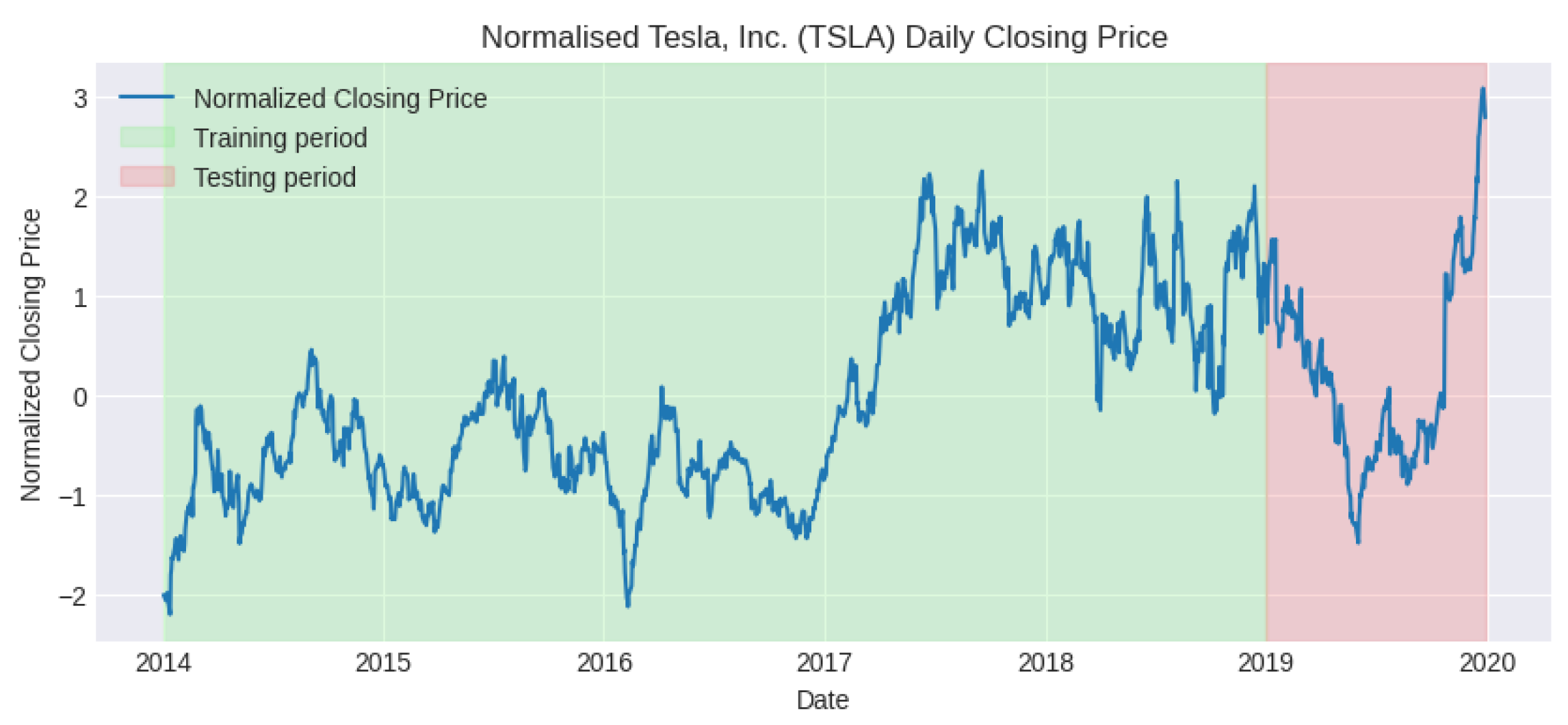
As seen in Figure 1, the training data consists of normalised daily closing prices for 5 years, spanning from 1 January 2014 to 1 January 2019, while the testing data consists of daily closing prices for 2019. We curtailed the testing dataset to prevent the inclusion of anomalies arising during the COVID-19 pandemic.
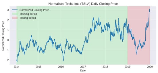
Figure 1.
Graph showing train–test split of normalised Tesla closing price, 2014–2020. Source: [30].
4.1.2. Financial Statements
Our approach to enriching state representation takes place through the analysis of financial statements. For this work, we focused specifically on Tesla’s 10-K and 10-Q reports submitted over the training and testing periods. Such reports, filed with the Securities and Exchange Commission (SEC), provide a comprehensive summary of a company’s financial performance [31]. A total of 24 such documents from Tesla were retrieved from the SEC’s public database. An example of the financial report can be seen in Appendix A.3.
4.1.3. Loughran–McDonald Sentiment Word Lists
For this task, we used the Loughran-McDonald sentiment word lists to construct a sentiment space [32]. The Loughran–McDonald sentiment word lists serve as a specialised lexicon that is leveraged for financial-text analysis through the inclusion of a list of words typically seen within financial documents. The list, sourced from [33], contains 85,221 words which are ranked in the following categories: “Negative”, “Positive”, “Uncertain”, “Litigious”, “Constraining”, “Superfluous”, “Interesting” and “Modal”. For the purpose of this study, we reduced the scope to focus on six sentiment categories that are the most relevant to our analysis, namely “Negative”, “Positive”, “Uncertain”, “Litigious”, “Constraining” and “Interesting”. Using these sentiments, we construct a multidimensional sentiment space, Appendix A.4, where each dimension represents a distinct sentiment category, providing a more intuitive interpretation of the document’s sentiment content.
4.1.4. Cosine Similarity
Using the Loughran–McDonald sentiment word lists as terms in the TF-IDF vectoriser, we generated TF-IDF scores only for these sentiment-signifying words across all the 10-K and 10-Q documents. The formula used for calculating the TF-IDF is as follows:
where is the TF-IDF score of the jth sentiment word in the ith document, is the term frequency, which is the number of occurrences of the jth sentiment word in the ith document, and is the number of documents within the corpus that contain the jth sentiment word. The denominator of the logarithmic term contains a smoothing factor of +1 to ensure that the inverse document frequency (IDF) score is always defined and positive.
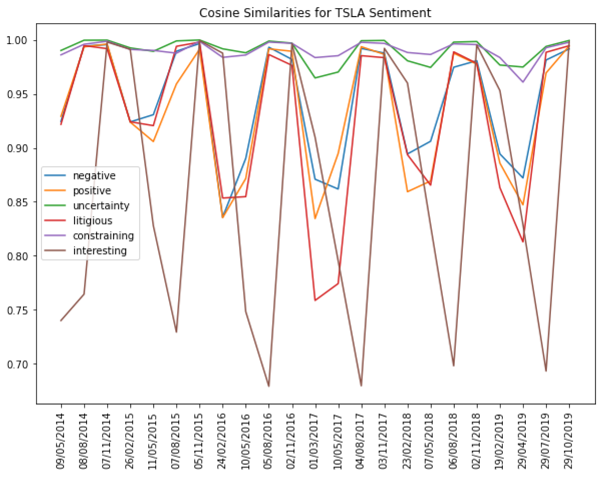
After the TF-IDF scores had been obtained, the cosine similarities were calculated for each neighbouring TFIDF vector/document. The cosine similarity between two vectors is defined as , where u and v are the two vectors of comparison. The resulting value represents a score highlighting the similarity across consecutive 10-k and 10-q documents, achieved by measuring the cosine between two vectors within multi-dimensional space, with a score of 1 claiming two identical vectors and a score of −1 claiming that two vectors are diametrically opposed. A score of 0 suggests that the two vectors are orthogonal, meaning that the documents have no common terms.) The results are evidenced in Figure 2.

Figure 2.
Cosine similarity scores for TSLA sentiment, 2014–2020. Source: [30].
4.2. Experiment
Two environments were examined, namely a conventional trading environment and an augmented trading environment where sentiment analysis data were incorporated into each state representation. The objective of this comparison was to assess the impact of sentiment analysis data on the trading decisions and overall performance of the agent. Alongside the environments, various look-back windows were experimented with to determine the optimal number of past trading days the agent should consider when deciding on an action.
4.3. Environment
The CustomTradingEnvironment was implemented in a Python class, which was inherited from the gym.Env class provided via the OpenAI Gym framework [34]. This class consisted of two primary methods: reset and step.
- reset: This method is called when the environment is initialised or reset. It resets the environment to its initial state at the beginning of each episode.
- step: This method executes a time step in the environment. It takes an action as a parameter, updates the agent’s position, calculates the corresponding reward, transitions the environment to its next state and returns four values:
- –
- obs: the new state constructed by the get_observation method.
- –
- reward: a numerical reward for the action taken.
- –
- done: a boolean indicating whether the environment has reached a terminal state.
- –
- info: an info dictionary which can contain any auxiliary diagnostic information.
4.3.1. Constructing State
In our proposed trading environments, the get_observation method is called at each time step. This function is responsible for creating a state that represents the recent history of the Tesla stock within the specified look-back window. Each state, , thus represents a snapshot of the past and current market conditions.
In addition to the past window of stock price data and 5 technical indicators, Appendix A.2, the state space includes the current position held by the agent in the stock market, the day of the week, and, in the augmented environment, sentiment analysis data. The final features included in the conventional environment’s state space can be represented as follows:
where C is the closing price of the Tesla stock, i is the current time step, L is the length of the lookback window, is the day of the week, is the position currently held by the agent in the market, and , , , and are a set of technical indicators whose descriptions can be found in Appendix A.2.
In the augmented environment, we also integrated sentiment analysis data into the state space. As discussed earlier, we included the cosine similarity scores, derived from the sentiment analysis, for the following sentiment categories: “Negative”, ; “Positive”, ; “Uncertainty”, ; “Litigious”, ; “Constraining”, ; and “Interesting”, . Thus, the state space array for the augmented environment was structured as follows:
The augmented environment thus comprises a total of 14 features in the state space. To ensure that all features may contribute to the model’s performance, all features in the window were normalised to a common scale. As seen in Figure 1, the closing stock price data were normalised using z-score normalisation to adjust the values in the dataset to a common scale without distorting the differences in the ranges of values or losing information. The z-score is calculated as , where X is the original data point, is the mean of the data, and is the standard deviation of the data.
4.3.2. Update Positions
In our CustomTradingEnvironment class, we introduced a ”position” instance variable. This variable keeps track of the agent’s current position, with {1, -1, 0} representing long, short and no positions, respectively.
The process of updating the position in our trading environment starts with retrieving the state array from the get_observation method. The state array is then reshaped to fit the input requirements of our LSTM network, which takes the shape of a three-dimensional array defined by the following dimensions: (batch_size, time_steps and features). The batch size and time step are two of the hyperparameters tuned in Section 4.7, which also contribute to the Q-network’s input dimentionality, while the three linear output neurons of our Q-network are intrinsic to our system’s design—each representing the Q-value of a given action [35].
These neurons produce an estimated action value, , for each of the three possible actions, , where is the set of network weights after k updates. These action-value estimates are then fed through an -greedy action selection mechanism which selects the action for step t as either or, with a probability of , a random exploratory action, .
This action selection process forms our action space, , , which was discretised to these three action signals {0, 1, 2} representing hold, buy and sell, respectively [35]. The action signal is then passed to the environment, which updates the agent’s position in the stock market, as illustrated in Table 1 below.

Table 1.
Interpretation of each action signal, .
The method of discretisation aligns well with our trading framework. The trading system focuses primarily on deciding optimal times to open or close positions, rather than their size. Thus, the actions can be discretised into simple dichotomies of buy/sell/hold.
4.4. Reward Function Design
Percentage PnL
The most intuitive approach was to use the percentage PnL as the primary reward function in our trading environment. The percentage PnL gives the percentage returns from each trade based on the change in the raw stock price, as opposed to the normalised price used in the observation space.
The calculate_reward method in the CustomTradingEnvironment computes the percentage price change for each trade based on the exit and the entry price and then multiplies it with the agent’s position. This is so that, if the agent was holding a short position (−1) and the exit price, , is lower than the entry price, , then the agent is rewarded with a positive reward, and vice versa.
Furthermore, we modelled the reward function to calculate the trading fee only if a position has been taken or closed; i.e., if the agent chooses to hold a position, the reward is calculated without the trading fee. The complete and final reward function scheme can be expressed as follows:
where is the current price, is the previous price, is the entry price, is the exit price, “p” is the current position held by the agent—long (1), short (−1) or no position (0)—and “a” is the action selected by the agent—hold (0), buy (1) or sell (2).
4.5. Agent
The agent’s architecture is predominantly defined by its underlying Q-network. As mentioned in Section 3, this network is tasked with computing a function, , which maps a given state to Q-values for each action that can then be selected based on the policy. The final Q-network configuration is summarised in Table 2 and Table 3 as follows:
Table 2.
Architecture of the Q-network.
Table 3.
Properties of the Q-network.
4.6. Algorithm
As detailed in Section 3, the agent is trained using a variant of Q-learning known as Double Deep Q-Learning, an extension of the Deep Q-Learning algorithm that reduces the overestimation bias of Q-values. The DDQN with its properties is, therefore, considered the core of the RL framework, and the following Algorithm 1 describes the process adapted to our case [7]:
| Algorithm 1 Double Deep Q-Learning (Hasselt et al., 2016) |
|
4.7. Hyperparameters
In order to compare the performances, we kept the same hyperparameters for both environments. The exploration probability is defined by a function where decreases at a specified decay rate, , from 1.0 to . All key parameters are summarised in Table 4 and Table 5, and their descriptions can be found in Appendix A.5.
Table 4.
DDQN agent training hyperparameters: values.
Table 5.
DDQN agent training hyperparameters: values.
4.8. Training Procedure
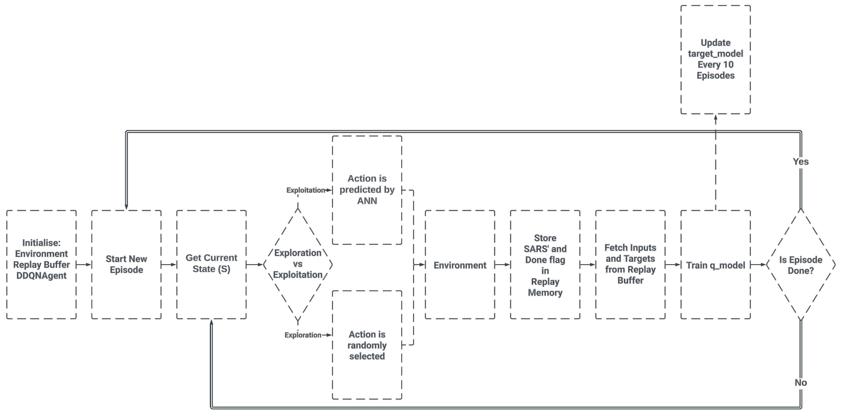
The procedure for training the RL agent is the same for both environments. The complete training procedure can be summarised as per Figure 3.
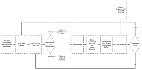
Figure 3.
Training procedure schema. Source: own.
5. Results
This section showcases the application of the trained agent to our custom environments. The results, obtained with varying look-back windows and an augmented state space, offer insights into the agent’s sensitivity to these design choices. In order to ensure a valid test simulation, the DDQN agent should not benefit from hindsight or look-ahead bias. This is achieved by only giving the agent access to information that would have been available at the time of the trading decisions, ensuring that the agent’s performance on the test set is representative of its true capability.
5.1. Evaluation Metrics
To evaluate the performance of our trading system under the various design choices, we chose to use the following evaluation metrics:
- Cumulative return: The first metric is a measure of the total profit or loss that our model is able to achieve over the duration of the testing period. It provides an indication of the model’s ability to maximise returns and, thus, the effectiveness of its trading decisions.
- Benchmark comparison: The second metric involves benchmarking the model’s learned trading strategy against a buy-and-hold strategy, where one holds onto a stock throughout a given period. Using this as a benchmark, we can assess whether our DRL agent’s trading strategy can lead to alpha (excess return) over simply investing in the market and holding.
- Calmar ratio: The third metric is the Calmar ratio, which is used to determine the financial efficiency of our trading system. It is calculated as the ratio of the annualised return to the maximum drawdown during the testing period [36]. This metric allows us to compare the risk-adjusted returns of our model’s strategy with those of the ”buy and hold” strategy.
5.2. Conventional Environment
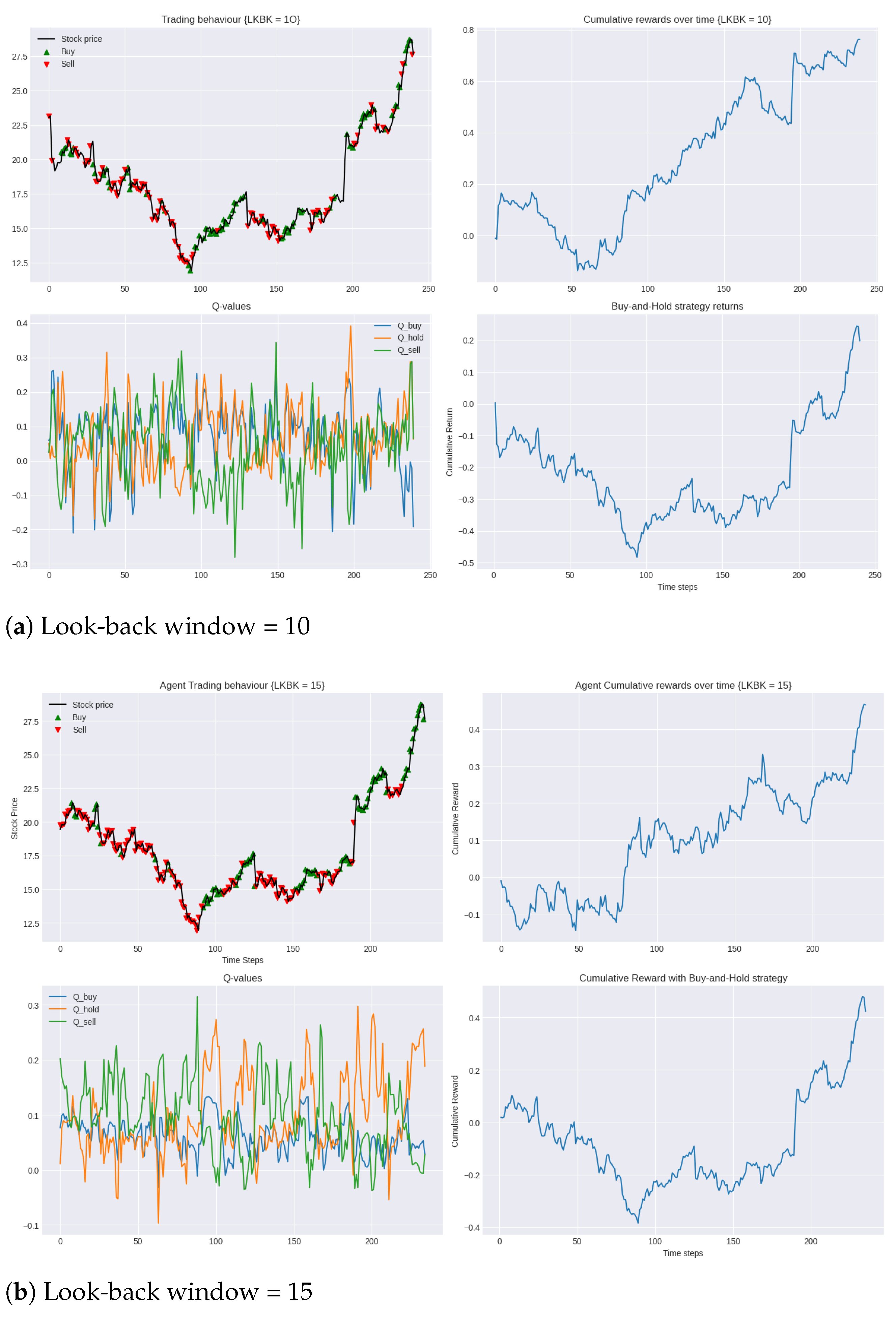
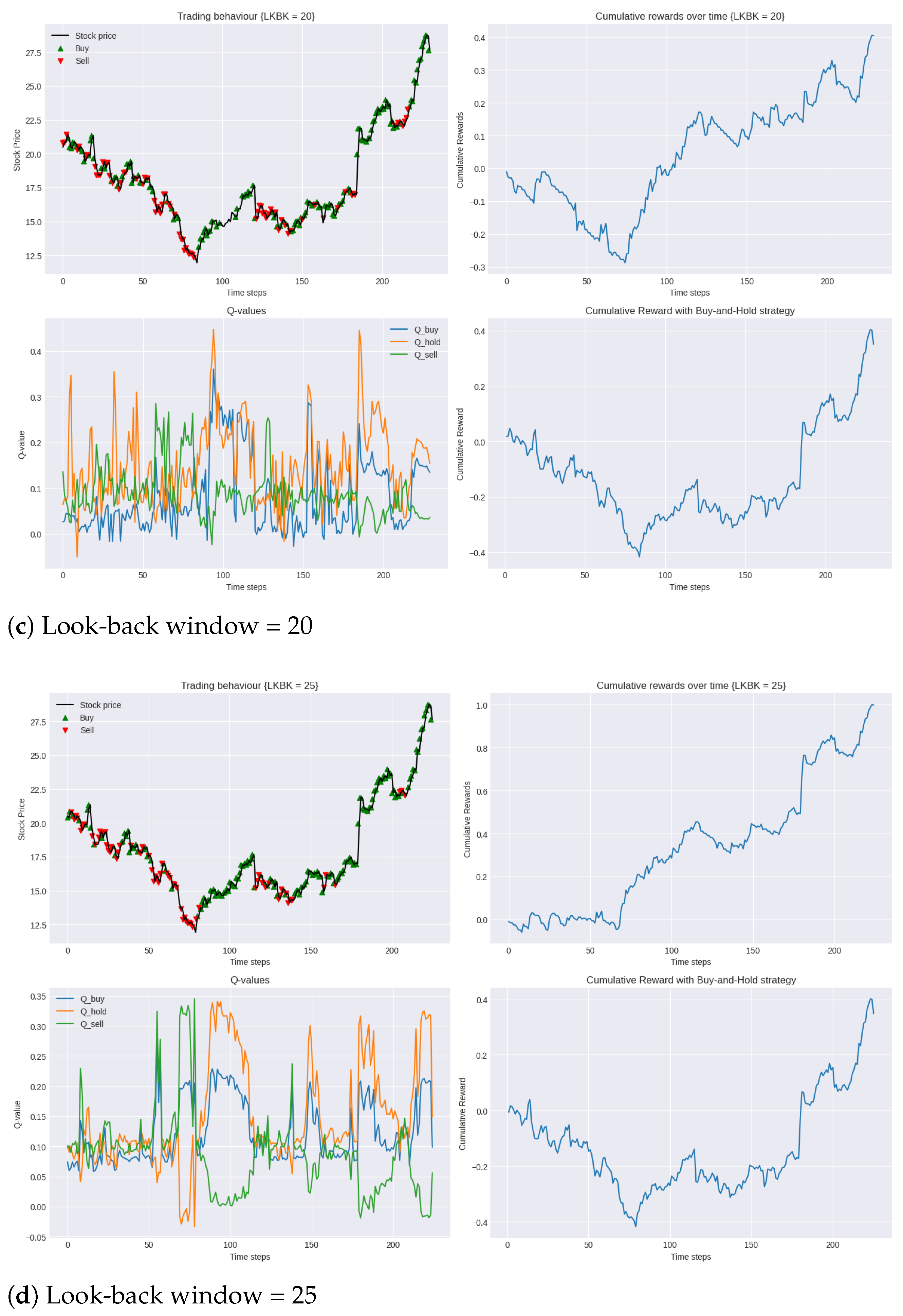
Figure 4 presents the performance of the system’s trading behaviour during the testing period compared to the market (buy-and-hold strategy). The results show the agent’s ability to make trading decisions with the unseen test data in 2019, demonstrating the generalisation power of the optimal policy it learned after training for 50 episodes with the 2014–2019 training data. The green and red arrows represent long and short positions, respectively.
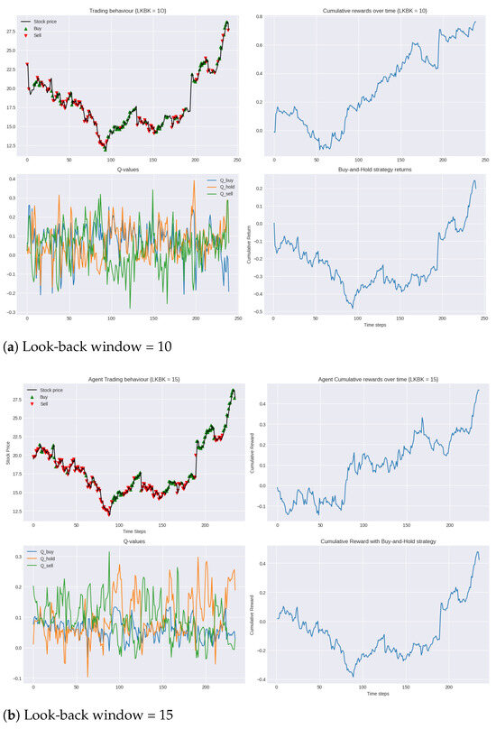
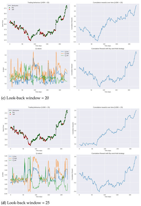
Figure 4.
Performance of DDQN in testing period 2019 compared to buy-and-hold strategy for varying lengths of look-back windows.
During the testing phase, we can see that, in all models, generally, the agent is able to correctly identify suitable timings for both opening and closing positions, both long and short. Despite the negative cumulative rewards observed in the opening 50 trading days, the agent is able to consistently outperform the benchmark set with the simple buy-and-hold strategy by a significant margin, validating the efficacy of the agent’s learnt policy.
A particular highlight is seen with the 25-day look-back window, as shown in Figure 4d. Here, the agent not only limits the initial losses but also achieves the highest overall reward. This shows that the agent’s learnt policy in this model is not only the most robust to unfamiliar market dynamics and volatility but also the most profitable.
As described in Section 5.1, an essential next step in the evaluation process is to assess the financial efficiency (the ratio of profits to risk) of our trading system using the Calmar ratio. In this set of experiments, the 25-day look-back window achieved the highest Calmar ratio of 0.9, while the 15-day look-back window had the lowest at 0.3. Nonetheless, both of these results surpassed the Calmar ratio of the buy-and-hold strategy of 0.2, also demonstrating the superior risk-adjusted performance of our agent.
In analysing the Q-values over the testing period, we observed that the use of a Double Deep Q-Network also resulted in a clear differentiation in Q-values corresponding to the buy, hold and sell actions, highlighting the agent’s clarity in decision-making. We further observed that this separation grew as the look-back window increased. The correlation with look-back window length and Q-value separation suggest that the agent is more certain of its decisions when it is able to look at a longer window of past market data before it makes its decision.
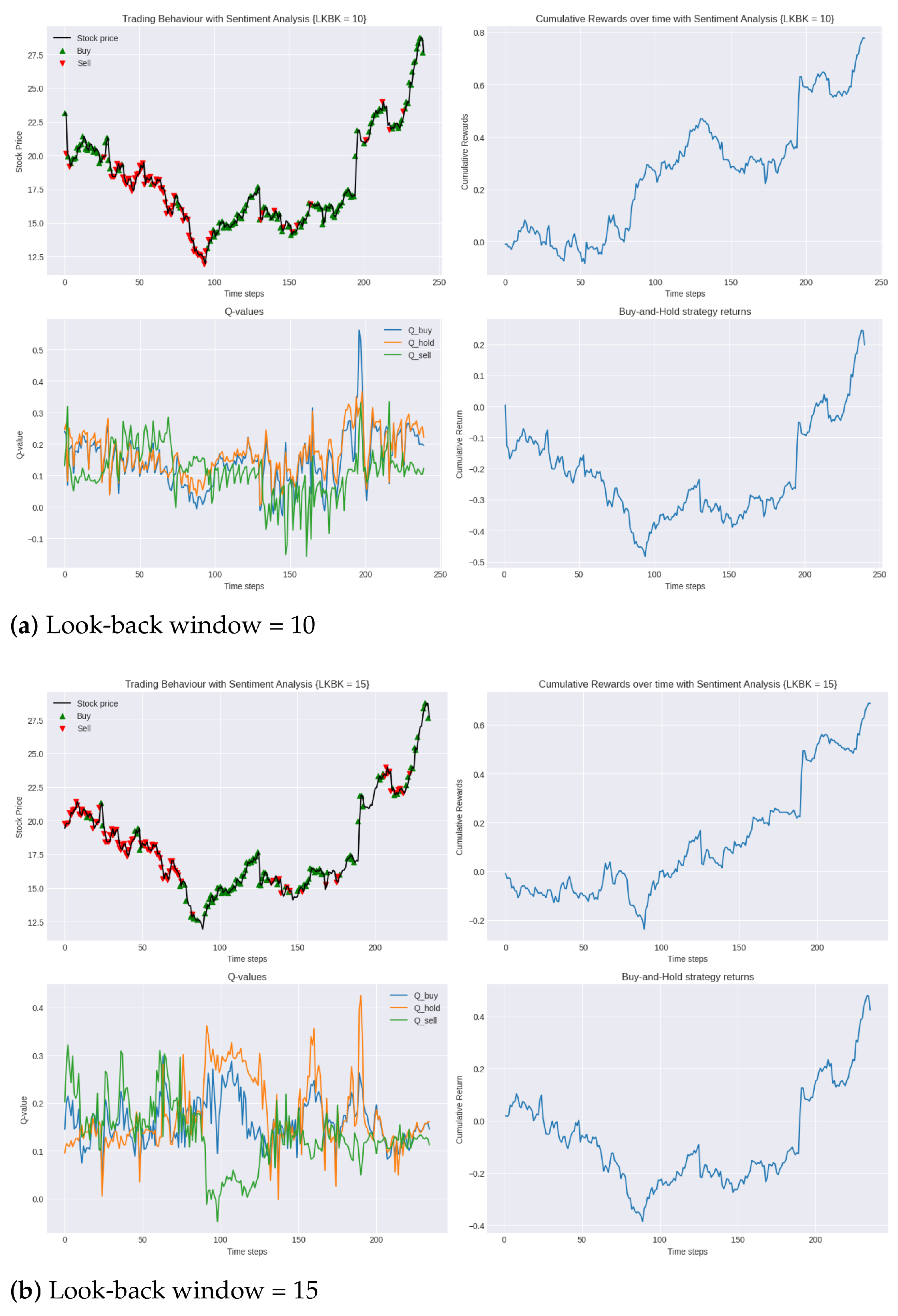
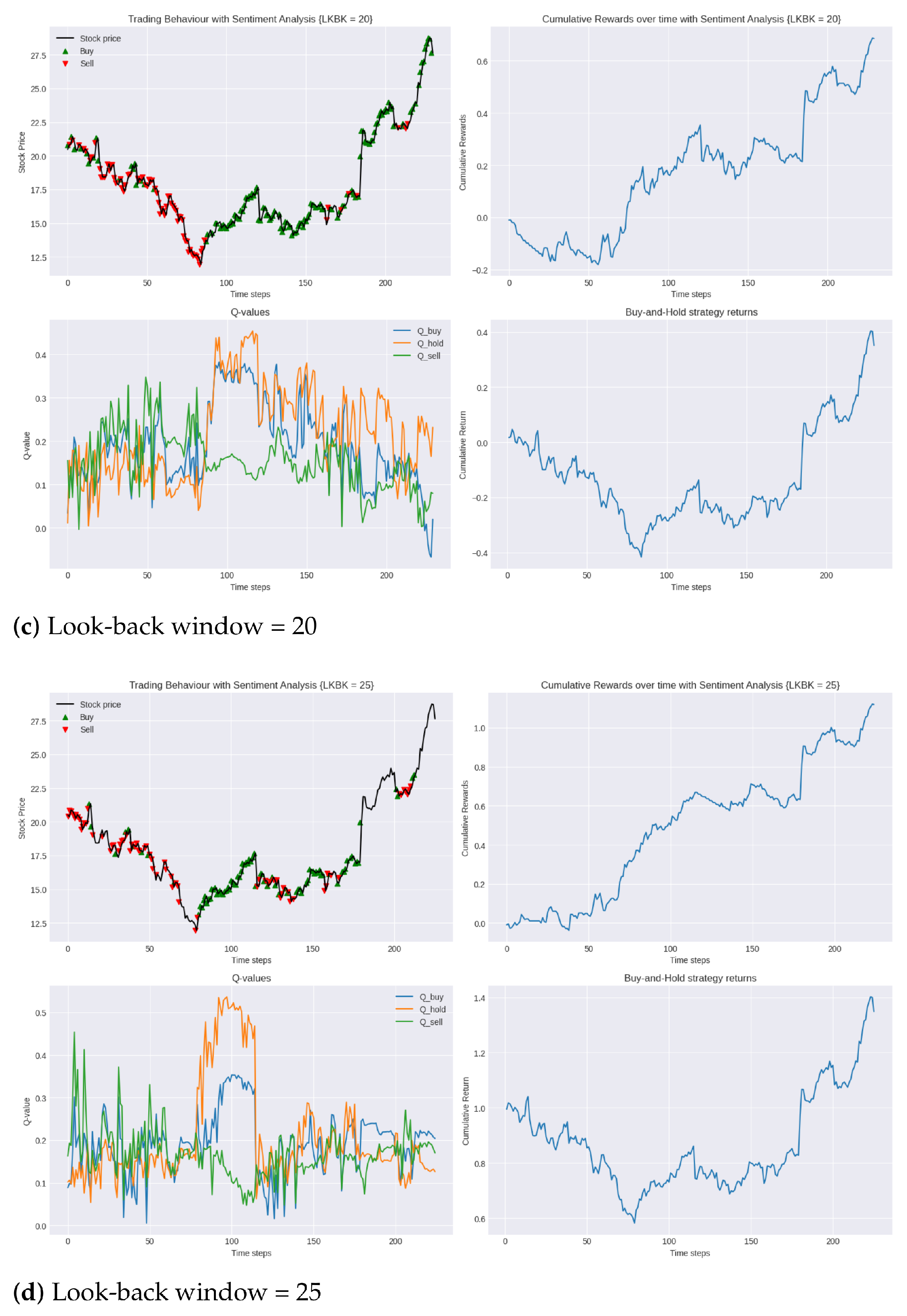
5.3. Environment Augmented with Sentiment Analysis
In this enhanced trading environment, we can see that the incorporation of sentiment analysis into the state space has undeniably enhanced the agent’s performance. As seen in Table 6, comparing the performance of the agent in the two environments for each look-back window, we can see that the agent’s optimal policy was consistently more profitable in the second environment. In the augmented environment, the agent was able to increase its cumulative reward in the testing period by up to 70%. This not only indicates that the use of sentiment analysis allows the agent to make better predictions of the stock price evolution but also helps the agent converge to a policy that is more robust to new market dynamics and, thus, has more generalisation power. This notion is further emphasised in Figure 5a,b,d where, compared to the conventional environment, for the same look-back window length, the agent’s policy is able to significantly minimise the loss incurred in the opening 50 trading days.
Table 6.
Comparison of total rewards accumulated over test period in different environments.
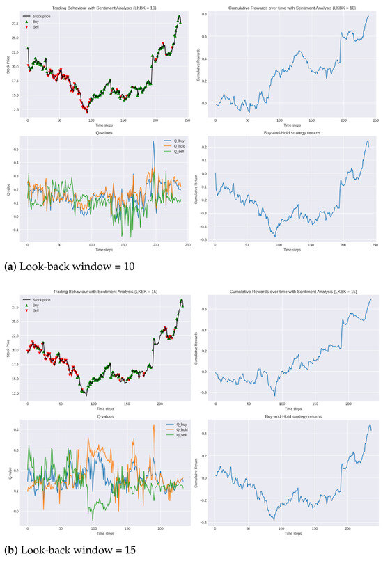
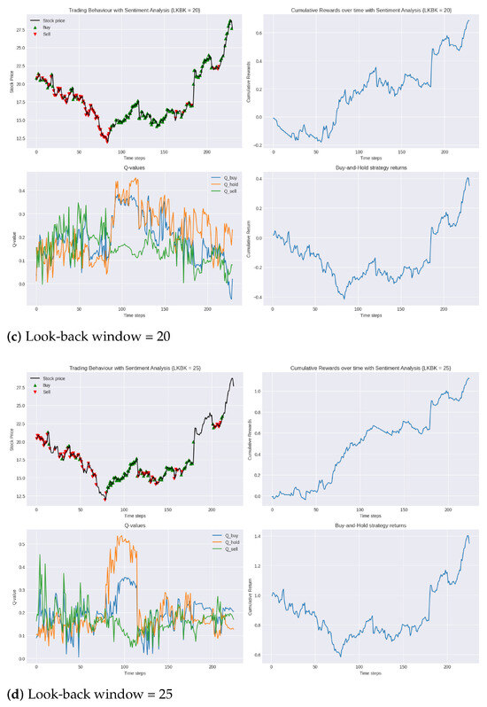
Figure 5.
Performance of DDQN with sentiment analysis in testing period 2019 compared to buy-and-hold strategy for varying lengths of look-back windows.
To quantify the profit-to-loss ratio, we again turned to the Calmar ratio. In this set of experiments, the 25-day look-back window achieved the highest Calmar ratio of 1.3, while the 15-day look-back window had the lowest at 0.5. These results show a significant improvement in the financial efficiency of our trading model, with the inclusion of sentiment analysis raising the highest Calmar ratio achieved with the model from 0.9 to 1.3.
Interestingly, similar to observations found in the conventional trading environment, the results do not display a clear linear relationship between the length of the look-back window and trading performance. Specifically, following the 25-day window’s strong performance, the 10-day window, as evidenced in Figure 5a, demonstrates superior performance over the longer 20-day window, depicted in Figure 5c. Such findings further highlight the inherent complexities of trading environments and the challenge in obtaining a singular optimal strategy.
6. Discussion
This paper has presented a Double Deep Q-Learning approach to algorithmic trading, exploring the potential to enhance the state-space representation with additional features beyond price-based data. Furthermore, an investigation was carried out to determine the optimal number of days’ worth of previous market data that the agent should observe in the state space when deciding on an action to take. This is known as the look-back window. In this regard, eight models were evaluated and compared; the performance of each model, with lookback window lengths of 10 days, 15 days, 20 days and 25 days, was evaluated in both the conventional environment and in an environment augmented with sentiment analysis. The models were trained and tested in environments that simulated the stock market, including transaction costs where positions were taken or liquidated. The models were trained for 50 episodes with training data consisting of normalised daily closing prices for 5 years, spanning from 1 January 2014 to 1 January 2019, and sentiment analysis of Tesla’s 10-K and 10-Q reports, submitted over this period in the augmented environment. While trading, we will never see the same exact state twice, so the power of generalisation is essential. Therefore, the agent’s architecture was designed to balance the learning capability and model complexity to ensure that the network was capable of learning without memorising the training data. We evaluated the performance of the models in trading the Tesla, Inc. (TSLA), stock in the period of 2 January 2019–31 December 2019, using the cumulative reward as the performance metric and the buy-and-hold strategy as the benchmark. All in all, the results of our experimentations were promising. Not only was our DDQN agent able to learn a profitable trading strategy that was robust to the volatility of unfamiliar market dynamics in 2019 but every model was also able to surpass the benchmark set in the simple buy-and-hold strategy, further attesting to the potential and efficacy of applying RL to the financial domain. In our efforts to determine the optimal period length from which the agent references past data to make its current decisions, a 25-day look-back window emerged as the most favourable in terms of the agent’s overall performance. However, what became clear through our experimentation with this parameter was the absence of a clear correlation between the length of the look-back window and the resulting performance. This, however, does leave room for further work. Researchers could analyse a wider range of look-back window durations, perhaps in smaller increments, to establish a clear relationship.
One of the notable achievements of our research was the incorporation of sentiment analysis into our agent’s trading strategy, through which we witnessed up to a 70% increase in the cumulative reward over the testing period. As discussed in Section 2, very few studies found in the literature incorporated non-price-based features in the agent’s state representation. These positive results provide a compelling illustration of the potential of including additional data sources of information in the state representation beyond just historical price-based data.
While our research provides valuable insights and demonstrates the potential of DDQN in stock market trading, it also unveils avenues for further exploration and refinement. In line with our findings, the following potential future work can be considered:
- The agent’s policy was evaluated on the 2019 Tesla stock data. An essential next step would be to evaluate the policy’s generalisation capability with a diverse set of stocks in the technology sector (e.g., Apple, Microsoft and Amazon), extending the target from trading a single asset to selecting from multiple assets.
- Additionally, exploring the application of this approach in other markets, such as the foreign exchange market, could further validate the robustness and versatility of the model.
- While our agent processed sentiment from Tesla’s 10-K and 10-Q reports, incorporating sentiment derived from news articles or social media platforms like Twitter could provide the agent with a broader perspective.
- While our current agent works with discretised actions, focusing primarily on deciding optimal times to open or close positions, a more granular approach could use a continuous action space. This would allow the agent to factor in considerations like the proportion of capital to invest each time it opens a position.
7. Conclusions
In conclusion, we have demonstrated a significant advancement in the field of algorithmic trading through the implementation of a Double Deep Q-Learning (DDQN) model enhanced with sentiment analysis. The DDQN algorithm has been validated by many researchers as the state-of-the-art technique in applying value-based reinforcement learning to finance, noted for its improved learning stability and estimation capabilities, compared to the former DQN model. Our research not only corroborates these strengths but also illustrates a substantial enhancement in performance when the model’s state space is augmented with sentiment scores derived from financial reports. As hypothesised, the incorporation of sentiment analysis into the DDQN’s state space allowed for a more holistic view of the market conditions, acknowledging that factors beyond historical price data can significantly influence trading decisions. Our goal was to allow the agent to emulate the decision-making process of a real-life trader who would typically conduct fundamental analysis to make trading decisions on a particular stock. This approach led to a 70% increase in the cumulative reward over the testing period and a Calmar ratio increase from 0.9 to 1.3, significantly outperforming the benchmark buy-and-hold strategy. These improvements not only demonstrate the enhanced profitability of our trading system but also, more importantly, the increase in the Calmar ratio indicates improved financial efficiency, accounting for the risk associated with the agent’s trading strategy. Such results highlight the potential of integrating alternative data sources into the state space, a method often overlooked in reinforcement learning research within the financial sector.
This study not only reinforces the efficacy of DDQN in the trading domain; also, the significant improvements observed with the inclusion of sentiment analysis in our study highlight the importance and impact of expanding the agent’s state space representation beyond conventional data types, thereby setting a new benchmark for future research in reinforcement learning applications in finance.
Author Contributions
Conceptualization, L.T. and J.M.V.K.; methodology, L.T. and J.M.V.K.; software, L.T.; validation, L.T. and J.M.V.K.; formal analysis, L.T., J.M.V.K. and A.J.R.-S.; investigation, L.T., J.M.V.K. and D.M.-V.; resources, L.T. and P.J.E.-A.; data curation, L.T. and J.M.V.K.; writing—original draft preparation, L.T. and J.M.V.K.; writing—review and editing, L.T.; visualization, L.T., J.C.S.-R., E.R.-D. and D.M.-V.; supervision, P.J.E.-A. and A.J.R.-S.; project administration, J.C.S.-R. and E.R.-D. All authors have read and agreed to the published version of the manuscript.
Funding
This research received no external funding.
Institutional Review Board Statement
Not applicable.
Informed Consent Statement
Not applicable.
Data Availability Statement
All research data are available in References at [30,31,32,33,37,38].
Conflicts of Interest
The authors declare no conflicts of interest.
Appendix A. Data Analysis and Pre-Processing
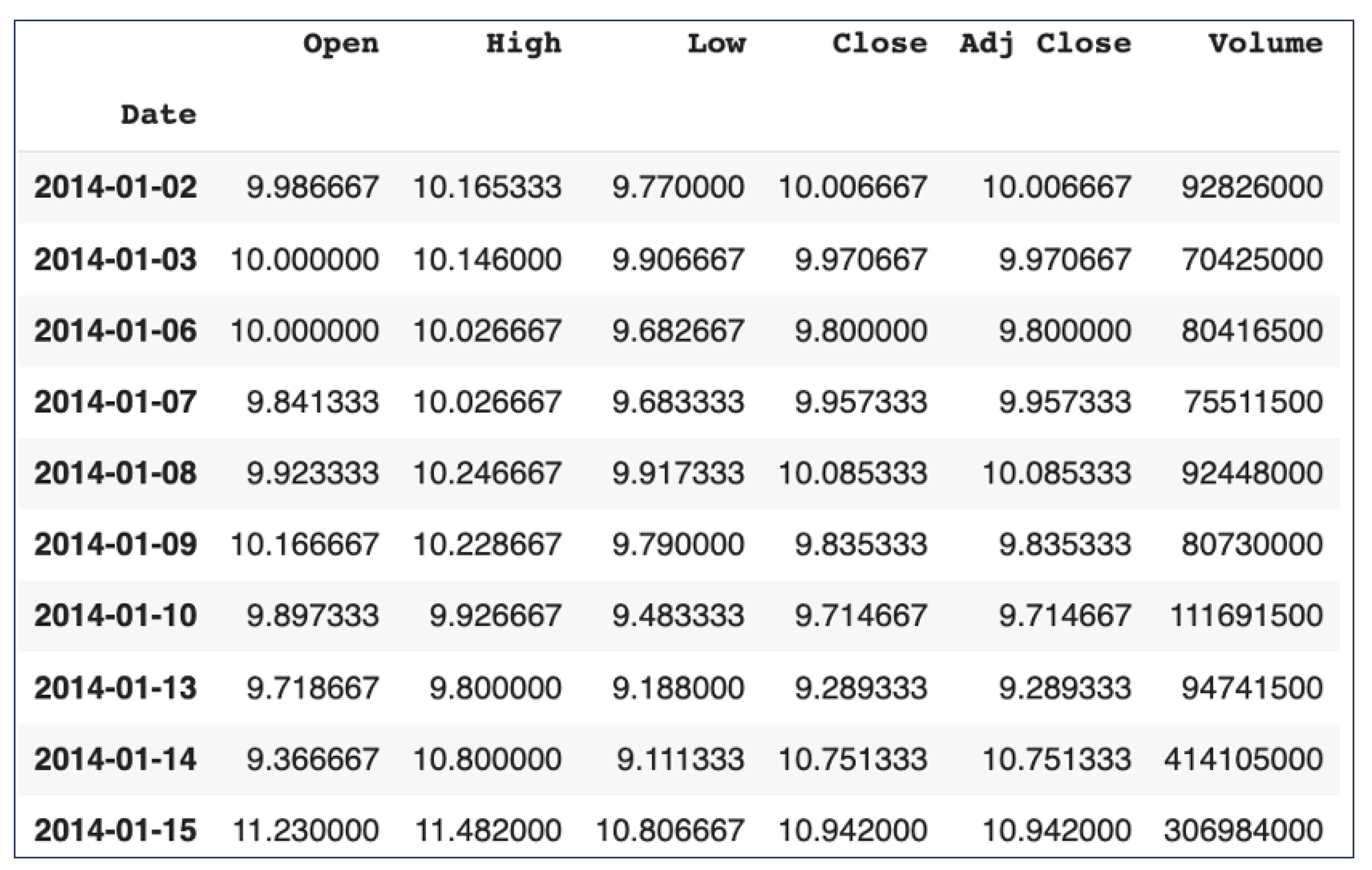
Appendix A.1. Tesla Stock Data
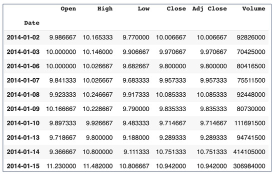
Figure A1.
Segment of Tesla stock OHLCV data. Source: [30].
Figure A1.
Segment of Tesla stock OHLCV data. Source: [30].
Appendix A.2. Technical Indicators
Table A1.
Description of technical indicators. Source: [39,40,41,42,43,44].
Table A1.
Description of technical indicators. Source: [39,40,41,42,43,44].
| Indicator | Description | Formula |
|---|---|---|
| SMA (simple moving average) | Average of prices over periods | SMA = |
| RSI (relative strength index) | Speed and change of price movements | RSI = |
| MOM (momentum) | Rate of rise or fall in prices | MOM = |
| BOP (balance of power) | Volume to price change | BOP = |
| AROONOSC (Aroon oscillator) | Trend-direction change identification | AROONOSC = |
| EMA (exponential moving average) | Weighted moving average | EMA = |
Appendix A.3. Financial Statements
Appendix A.3.1. Raw 10-K Segment
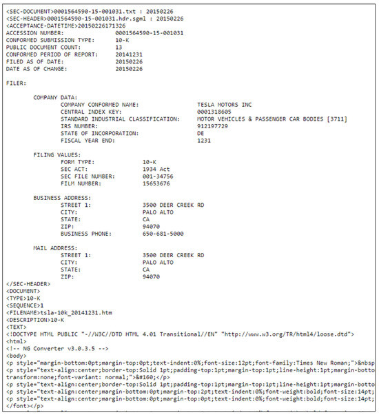
Figure A2.
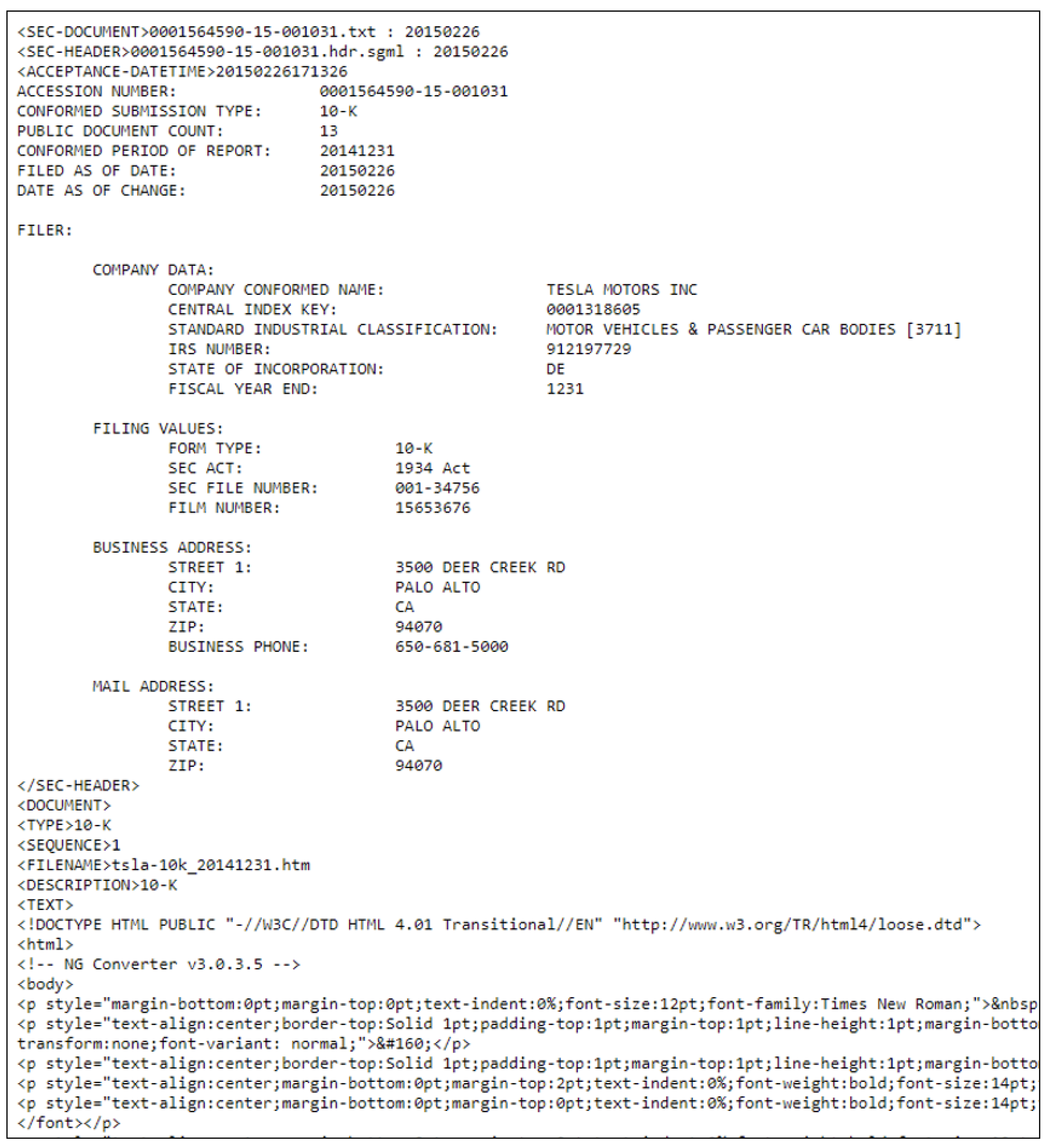
Segment of 2014 10-K raw .txt file. Source: [37].
Figure A2.
Segment of 2014 10-K raw .txt file. Source: [37].
Appendix A.3.2. Raw 10-Q Segment
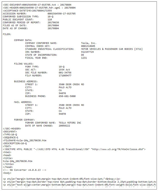
Figure A3.
Segment of 2017 10-Q raw .txt file. Source: [38].
Figure A3.
Segment of 2017 10-Q raw .txt file. Source: [38].
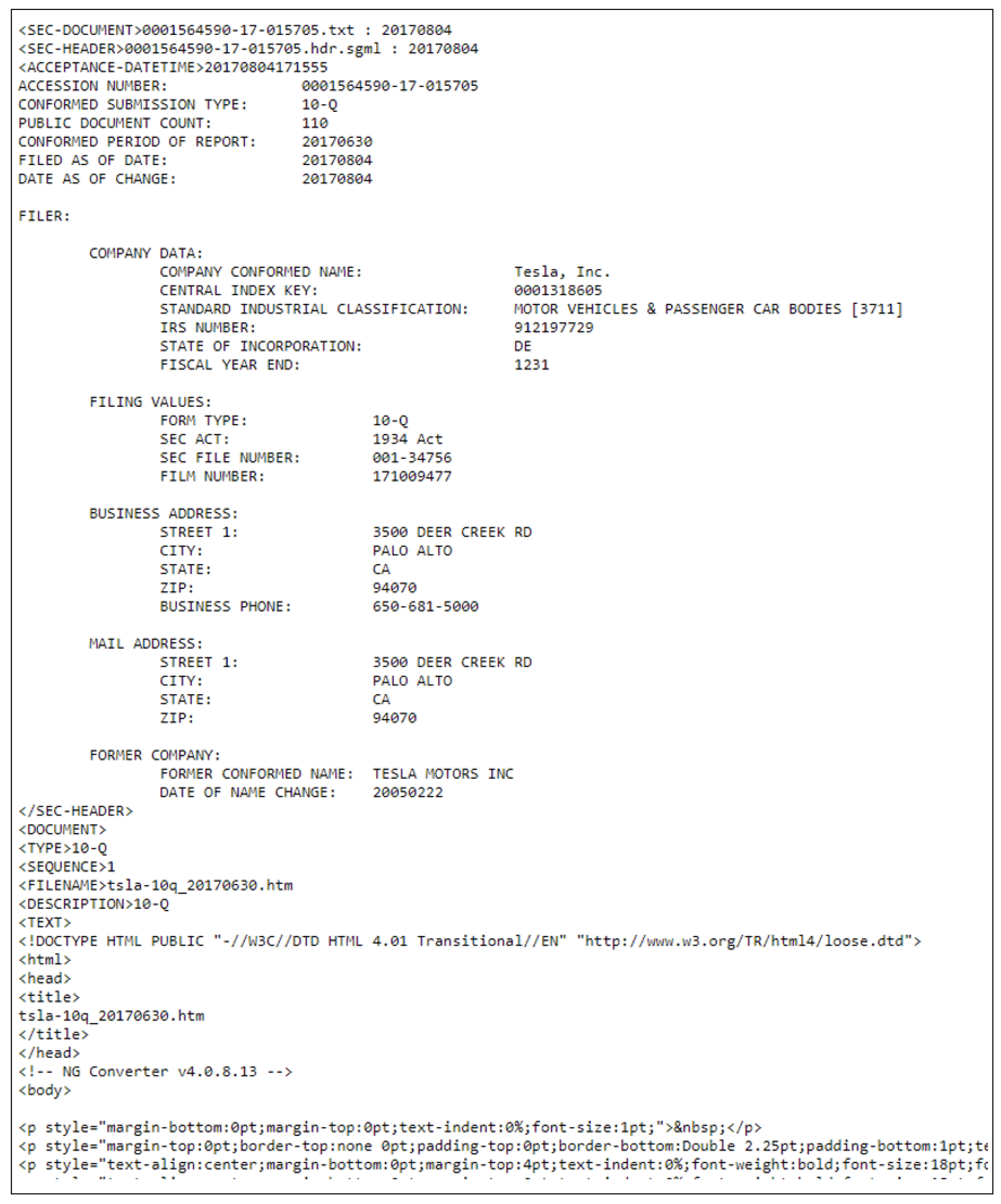
The 10-K is an annual report that includes information about a company’s operations, financial status and cash flow. The 10-Q is a quarterly report that provides an ongoing view of a company’s financial position during the year. The 10-Q is less detailed than the annual 10-K, but it does provide updated financial information throughout the year.
As seen in Figure A3, the data are extremely noisy. For example, the presence of HTML tags is one of the many unnecessary features of the text that make extracting sentiment from the documents impossible.
The document-cleaning procedure is described in the following steps:
- Isolate the ”document” section from the full text.
- Isolate the document according to its document ”type”, extracting the ”10-K” segment of the text.
- Parse through the 10-K segment, removing all HTML tags.
- Normalise the text, converting all the characters into lowercase format.
- Remove any present uniform resource locators (URLs) from the text.
- Lemmatise all the words within the text.
- Remove all present stop words within the text.
Table A2.
Raw vs. clean 10-K and 10-Q document file sizes in megabytes.
Table A2.
Raw vs. clean 10-K and 10-Q document file sizes in megabytes.
| Document Type | Raw File Size (MB) | Cleaned File Size (MB) |
|---|---|---|
| 10-K | 26.7 | 0.361 |
| 10-Q | 10.3 | 0.212 |
Appendix A.4. Sentiment Word List
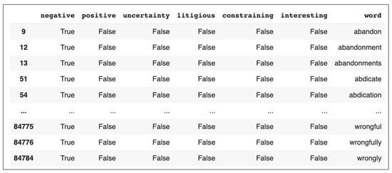
Figure A4.
Segment of sentiment space constructed using Loughran–McDonald sentiment word lists. Source: [33].
Figure A4.
Segment of sentiment space constructed using Loughran–McDonald sentiment word lists. Source: [33].
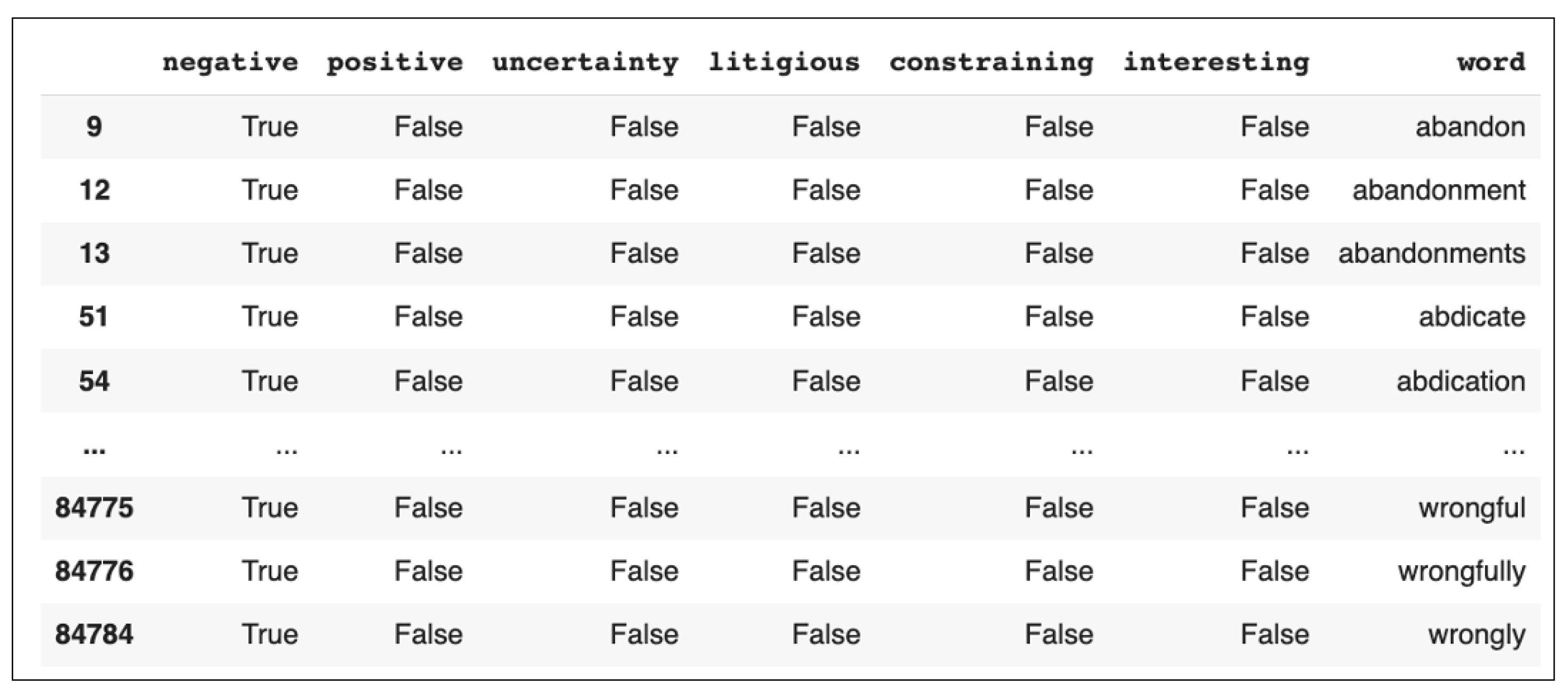
The 85,221 words within the lists were then normalised by converting all of them into lowercase, and they were lemmatised, followed by duplicate words being omitted.
Appendix A.5. DDQN Agent Training Hyperparameters: Descriptions
Table A3.
DDQN agent training hyperparameters: descriptions.
Table A3.
DDQN agent training hyperparameters: descriptions.
| Hyperparameter | Description |
|---|---|
| The discount factor used in the DDQL update. It determines how much future rewards contribute to the expected cumulative reward. We used a higher gamma value to give more importance to future rewards. | |
| The probability of taking a random action. Initially, this was set to a high value to encourage exploration, and then it decayed over time to encourage the exploitation of learned policy. | |
| The minimum epsilon value. This ensures that the agent continues to explore throughout its training. | |
| The rate at which epsilon is decayed. Faster decay results in faster exploitation of learned policy. | |
| replay_buffer.max_size | The maximum number of experiences stored in the replay buffer. Having more experiences to learn from generally results in better performance. |
| batch_size | The number of experiences sampled from the memory to train the network. Larger batch sizes generally lead to faster, more stable training, but they also use more memory. We found a batch size of 64 to effectively balance learning efficiency with computational costs. |
| n_episodes | The number of training episodes. Each episode is a complete game, from start to finish. We found 50 to be the smallest number of episodes needed for the algorithm to converge to a good policy. |
| time_skip | Defines the number of time steps to skip between states. This reduces the computational load and avoids the redundancy of information between states. |
| target_network update frequency | The frequency at which the target network weights are updated. |
| learning rate | Dictates the step size at each iteration while moving towards a minimum of the loss function. A smaller rate ensures more careful convergence, but at the cost of longer training times. |
References
- Chan, E. Quantitative Trading: How to Build Your Own Algorithmic Trading Business; Wiley Trading; Wiley: Hoboken, NJ, USA, 2009; ISBN 9780470466261. [Google Scholar]
- Chan, E. Algorithmic Trading: Winning Strategies and Their Rationale; Wiley Trading; Wiley: Hoboken, NJ, USA, 2013; ISBN 9781118460146. [Google Scholar]
- Zimmermann, H. Intraday Trading with Neural Networks and Deep Reinforcement Learning; Imperial College London: London, UK, 2021. [Google Scholar]
- Maven. Machine Learning in Algorithmic Trading, Maven Securities. 2023. Available online: https://www.mavensecurities.com/machine-learning-in-algorithmic-trading/ (accessed on 17 May 2024).
- Spooner, T. Algorithmic Trading and Reinforcement Learning: Robust Methodologies for AI in Finance. Ph.D. Thesis, The University of Liverpool Repository, Liverpool, UK, 2021. Available online: https://livrepository.liverpool.ac.uk/3130139/ (accessed on 17 May 2024).
- Bellman, R. A Markovian Decision Process. J. Math. Mech. 1957, 6, 679–684. [Google Scholar] [CrossRef]
- van Hasselt, H.; Guez, A.; Silver, D. Deep reinforcement learning with double Q-learning. arXiv 2016, arXiv:1509.06461. [Google Scholar] [CrossRef]
- Mnih, V.; Kavukcuoglu, K.; Silver, D.; Graves, A.; Antonoglou, I.; Wierstra, D.; Riedmiller, M. Playing Atari with deep reinforcement learning. arXiv 2015, arXiv:1312.5602. [Google Scholar]
- Zejnullahu, F.; Moser, M.; Osterrieder, J. Applications of reinforcement learning in Finance—Trading with a double deep Q-Network. arXiv 2022, arXiv:2206.14267. [Google Scholar]
- Aldridge, I. High-Frequency Trading: A Practical Guide to Algorithmic Strategies and Trading Systems; John Wiley & Sons: Hoboken, NJ, USA, 2013; Volume 604. [Google Scholar]
- Savcenko, K. The ‘A’ Factor: The Role of Algorithmic Trading during an Energy Crisis; S&P Global Commodity Insights: London, UK, 2022; Available online: https://www.spglobal.com/commodityinsights/en/market-insights/blogs/electric-power/110322-algorithm-trading-europe-energy-crisis (accessed on 25 July 2024).
- Fischer, T.G. Reinforcement Learning in Financial Markets—A Survey; FAU Discussion Papers in Economics; No. 12/2018; Friedrich-Alexander-Universität Erlangen-Nürnberg, Institute for Economics: Erlangen, Germany, 2018. [Google Scholar]
- Neuneier, R. Optimal asset allocation using adaptive dynamic programming. Advances in Neural Information Processing Systems. 1996, pp. 952–958. Available online: https://proceedings.neurips.cc/paper/1995/hash/3a15c7d0bbe60300a39f76f8a5ba6896-Abstract.html (accessed on 1 August 2024).
- Jin, O.; El-Saawy, H. Portfolio Management Using Reinforcement Learning; Working Paper; Stanford University: Stanford, CA, USA, 2016. [Google Scholar]
- Liang, Z.; Chen, H.; Zhu, J.; Jiang, K.; Li, Y. Adversarial deep reinforcement learning in portfolio management. arXiv 2018, arXiv:1808.09940. [Google Scholar]
- Ding, X.; Zhang, Y.; Liu, T.; Duan, J. Deep learning for event-driven stock prediction. In Proceedings of the Twenty-Fourth International Joint Conference on Artificial Intelligence, Buenos Aires, Argentina, 25–31 July 2015. [Google Scholar]
- Zhu, K.; Liu, R. The selection of reinforcement learning state and value function applied to portfolio optimization. J. Fuzhou Univ. (Nat. Sci. Ed.) 2020, 48, 146–151. [Google Scholar]
- Dai, S.X.; Zhang, S.L. An application of reinforcement learning based approach to stock trading. Bus. Manag. 2021, 3, 23–27. [Google Scholar] [CrossRef]
- Ning, B.; Lin, F.H.T.; Jaimungal, S. Double deep Q-learning for optimal execution. arXiv 2018, arXiv:1812.06600. [Google Scholar] [CrossRef]
- Machine Learning Trading. Trading with Deep Reinforcement Learning. Dr Thomas Starke (2020) YouTube. Available online: https://www.youtube.com/watch?v=H-c49jQxGbs (accessed on 2 February 2024).
- Nevmyvaka, Y.; Feng, Y.; Kearns, M. Reinforcement learning for optimized trade execution. In Proceedings of the 23rd International Conference on Machine Learning, ACM, Pittsburgh, PA, USA, 25–29 June 2006; pp. 673–680. [Google Scholar]
- Bertoluzzo, F.; Corazza, M. Testing different reinforcement learning configurations for financial trading: Introduction and applications. Procedia Econ. Financ. 2012, 3, 68–77. [Google Scholar] [CrossRef]
- Eilers, D.; Dunis, C.L.; von Mettenheim, H.-J.; Breitner, M.H. Intelligent trading of seasonal effects: A decision support algorithm based on reinforcement learning. Decis. Support Syst. 2014, 64, 100–108. [Google Scholar] [CrossRef]
- Sherstov, A.A.; Stone, P. Three automated stock-trading agents: A comparative study. In Proceeedings of the International Workshop on Agent-Mediated Electronic Commerce; Springer: Berlin/Heidelberg, Germany, 2004; pp. 173–187. [Google Scholar]
- Kaur, S. Algorithmic Trading Using Sentiment Analysis and Reinforcement Learning; Working Paper; Stanford University: Stanford, CA, USA, 2017. [Google Scholar]
- Rong, Z.H. Deep reinforcement learning stock algorithm trading system application. J. Comput. Knowl. Technol. 2020, 16, 75–76. [Google Scholar]
- Li, Y.; Zhou, P.; Li, F.; Yang, X. An improved reinforcement learning model based on sentiment analysis. arXiv 2021, arXiv:2111.15354. [Google Scholar]
- Pardo, R. The Evaluation and Optimization of Trading Strategies; John Wiley & Sons: Hoboken, NJ, USA, 2011. [Google Scholar]
- Hu, G. Advancing algorithmic trading: A multi-technique enhancement of deep Q-network models. arXiv 2023, arXiv:2311.05743. [Google Scholar]
- Tesla, Inc. (TSLA). Stock Historical Prices Data—Yahoo Finance—finance.yahoo.com. Available online: https://finance.yahoo.com/quote/TSLA/history?p=TSLA (accessed on 2 April 2024).
- SEC.gov—EDGAR Full Text Search—sec.gov. Available online: https://www.sec.gov/edgar/search/#/q=(Annual%2520report)&dateRange=all&ciks=0001318605&entityName=Tesla%252C%2520Inc.%2520(TSLA)%2520(CIK%25200001318605) (accessed on 2 May 2024).
- Marketing Communications: Web//University of Notre Dame Loughran-McDonald master Dictionary W/Sentiment Word Lists//Software Repository for Accounting and Finance//University of Notre Dame, Software Repository for Accounting and Finance. Available online: https://sraf.nd.edu/loughranmcdonald-master-dictionary/ (accessed on 2 May 2024).
- Loughran-McDonald Master Dictionary w/Sentiment Word Lists//Software Repository for Accounting and Finance//University of Notre Dame—sraf.nd.edu. Available online: https://sraf.nd.edu/loughranmcdonald-master-dictionary/ (accessed on 2 May 2024).
- Brockman, G.; Cheung, V.; Pettersson, L.; Schneider, J.; Schulman, J.; Tang, J.; Zaremba, W. OpenAI Gym. arXiv 2016, arXiv:1606.01540. [Google Scholar]
- Carapuço, J.M.B. Reinforcement Learning Applied to Forex Trading, Scribd. 2017. Available online: https://www.scribd.com/document/449849827/Corrected-Thesis-JoaoMaria67923 (accessed on 12 February 2024).
- Young, T.W. Calmar ratio: A smoother tool. Futures 1991, 20, 40. [Google Scholar]
- Edgar Filing Documents for 0001564590-17-015705. Available online: https://www.sec.gov/Archives/edgar/data/1318605/000156459017015705/0001564590-17-015705-index.htm (accessed on 2 May 2024).
- Edgar Filing Documents for 0001564590-15-001031. Available online: https://www.sec.gov/Archives/edgar/data/1318605/000156459015001031/0001564590-15-001031-index.htm (accessed on 2 May 2024).
- Murphy, J.J. Technical Analysis of the Financial Markets: A Comprehensive Guide to Trading Methods and Applications; Penguin Publishing Group: New York, NY, USA, 1999; 228p, Available online: https://www.google.com/books/edition/_/5zhXEqdr_IcC?hl=en&gbpv=0 (accessed on 24 July 2024).
- Wilder, J.W., Jr. New Concepts in Technical Trading Systems; Trend Research: Edmonton, AB, Canada, 1978; 6p, Available online: https://archive.org/details/newconceptsintec00wild/page/n151/mode/2up (accessed on 24 July 2024).
- Jahn, M. What Is the Haurlan Index? Investopedia. 2022. Available online: https://www.investopedia.com/terms/h/haurlanindex.asp#:~:text=The%20Haurlan%20Index%20was%20developed,the%20New%20York%20Stock%20Exchange (accessed on 24 July 2024).
- Ushman, D. What Is the SMA Indicator (Simple Moving Average). TrendSpider Learning Center, 2023. Available online: https://trendspider.com/learning-center/what-is-the-sma-indicator-simple-moving-average/ (accessed on 24 July 2024).
- Livshin, I. Balance Of Power. Tech. Anal. Stock. Commod. 2001, 19, 18–32. Available online: https://c.mql5.com/forextsd/forum/90/balance_of_market_power.pdf (accessed on 24 July 2024).
- Mitchell, C. Aroon Oscillator: Definition, Calculation Formula, Trade Signals, Investopedia. 2022. Available online: https://www.investopedia.com/terms/a/aroonoscillator.asp (accessed on 24 July 2024).
Disclaimer/Publisher’s Note: The statements, opinions and data contained in all publications are solely those of the individual author(s) and contributor(s) and not of MDPI and/or the editor(s). MDPI and/or the editor(s) disclaim responsibility for any injury to people or property resulting from any ideas, methods, instructions or products referred to in the content. |
© 2024 by the authors. Licensee MDPI, Basel, Switzerland. This article is an open access article distributed under the terms and conditions of the Creative Commons Attribution (CC BY) license (https://creativecommons.org/licenses/by/4.0/).