Abstract
In the early stages of residential project investment, accurately estimating the engineering costs of residential projects is crucial for cost control and management of the project. However, the current cost estimation of residential engineering in China is primarily carried out by cost personnel based on their own experience. This process is time-consuming and labour-intensive, and it involves subjective judgement, which can lead to significant estimation errors and fail to meet the rapidly developing market demands. Data collection for residential construction projects is challenging, with small sample sizes, numerous attributes, and complexity. This paper adopts a hybrid method combining a grey relational analysis, Lasso regression, and Backpropagation Neural Network (GAR-LASSO-BPNN). This method has significant advantages in handling high-dimensional small samples and multiple correlated variables. The grey relational analysis (GRA) is used to quantitatively identify cost-driving factors, and 14 highly correlated factors are selected as input variables. Then, regularization through Lasso regression (LASSO) is used to filter the final input variables, which are subsequently input into the Backpropagation Neural Network (BPNN) to establish the relationship between the unit cost of residential projects and 12 input variables. Compared to using LASSO and BPNN methods individually, the GAR-LASSO-BPNN hybrid prediction method performs better in terms of error evaluation metrics. The research findings can provide quantitative decision support for cost estimators in the early estimation stages of residential project investment decision-making.
1. Introduction
The current real estate industry faces challenges due to national policy regulations, the scarcity of land resources, and the continuous rise in land prices [1,2]. How to maintain profitability and reduce costs as much as possible has become a key issue for the development of enterprises. In residential construction projects, cost estimation is a crucial component, especially during the early decision-making stages, where it can have an impact on the total project cost of up to 75% to 95% [3]. During these early decision-making stages, cost estimation methods are largely based on past experiences and rely on cost engineers, requiring a high level of expertise. These methods also depend on certain survey and statistical data and often need to find completed projects with high similarity to the proposed project. Otherwise, issues such as insufficient design depth and low estimation accuracy may arise. In the late 20th century, in addition to experience-based methods, major companies began using static software tools such as Glodon, EXCEL, and SPSS for cost estimation. However, these programmes still cannot address complex pre-control cost issues like cost forecasting and require significant time and computational resources to complete the cost estimation [4]. Therefore, in response to the aforementioned research issues, there is an urgent need to establish an efficient, accurate, and quantifiable residential cost estimation model that can accurately estimate the cost of a new residential project within a short period. This model would improve the management and control of project costs, provide digital tools and technical support for real estate companies, and help them maintain competitiveness in a fiercely competitive market environment.
In recent years, project cost management has gradually transitioned from traditional static management to dynamic management. Many accumulated cost data have not been fully utilized, while advanced machine learning algorithm technologies can intelligently analyze historical data and estimate the costs of different types of construction projects based on initial project conditions. Currently, machine learning algorithms used for cost estimation in the construction field include multiple linear regression (MLR), Decision Tree (DT), Support Vector Regression (SVR), LASSO, and artificial neural networks (ANNs) [5,6,7], among which artificial neural networks are widely used [8,9]. Deepa et al. have identified the most influential factors in cost estimation models through investigations [10]. They combined the characteristics of artificial neural networks and engineering cost estimation to construct a hybrid cost estimation model based on neural networks. To overcome the slow convergence and low prediction accuracy of traditional ANN models, Ye applied the Backpropagation Neural Network (BPNN) to predict construction project costs, enhancing the network’s learning capability and robustness [11], providing a basis for cost management throughout the entire project lifecycle. Additionally, hybrid machine learning models such as Genetic Algorithm–Optimized Neural Networks (GA-BPNNs) have been used to accelerate model convergence and improve prediction accuracy [12,13]. Compared to traditional machine learning models, multiple linear regression may be affected by outliers and noise, especially with small datasets [14]. Decision Tree is sensitive to data changes, and their performance may be affected if the data change [15]. SVR is sensitive to the choice of kernel functions, and an inappropriate choice may lead to a decline in model performance [16]. LASSO regression, as a regularization method, shows unique advantages in a regression analysis. Its most significant advantage lies in feature selection and model optimization. By introducing the L1 penalty term, LASSO regression can automatically shrink the coefficients of irrelevant or redundant features to zero, achieving feature selection, making the model more concise and interpretable. Simultaneously, LASSO regression effectively addresses multicollinearity issues, enhancing the model’s stability and generalization ability, making it suitable for analyzing high-dimensional datasets in various fields [17,18,19]. Identifying important influencing factors of residential project costs is also crucial for predicting project costs [20]. Therefore, many scholars have conducted research on how to scientifically and effectively select feature factors for cost estimation and prediction. The screening methods mainly include GRA, questionnaire, sensitivity analysis, principal component analysis, factor analysis, and fuzzy analytic hierarchy processes [21,22,23,24,25]. Wang and Qiao considered the specificity and diversity of construction projects, noting that the factors influencing project costs are complex and varied. However, not all factors have the same weight and importance in project costs. Therefore, when selecting indicators, the principle of moderation should be considered. GRA can be used to screen out indicators that effectively describe the characteristics of the project or have a significant impact on project costs, which are then used for project cost prediction using the BiLSTM network [26]. GRA is a data analysis method based on grey system theory, aimed at studying the correlation between multiple indicators. It sums the data related to each indicator to determine the relative degree of each and calculates the grey correlation between indicators to determine the impact of each indicator on the issue. Compared to traditional correlation analysis methods, GRA can more accurately reflect the correlation and impact degree between indicators. Additionally, GRA has advantages such as a simple model, small data volume, and interpretable results [27], making it suitable for selecting residential project cost indicators in this study’s small dataset. Tong et al. quantitatively identified key cost drivers through GRA, selected relevant indicators as input variables, and then used LASSO regression to establish the relationship between engineering feature variables, economic factors, and highway engineering budgets [28]. Compared with LASSO regression without GRA, they found that the GRA-LASSO hybrid method was more accurate in predicting highway project costs. Yu et al. applied LASSO regression for factor selection and constructed a LASSO-BP hybrid model for short-term vegetable price prediction, resulting in an 82.11% lower prediction error compared to BPNN [29].
Based on the above research backgrounds, to improve the accuracy of residential unit cost predictions, this study combines the characteristics of cost data for residential projects, which are small in sample size and high-dimensional, with the advantages of LASSO regression and BPNN. This paper uses GRA to rank the correlation of input variables affecting the unit cost of residential projects, employs LASSO regression regularization and model evaluation for variable selection, and constructs a predictive ensemble model based on GRA-LASSO-BPNN. This model is compared with commonly used machine learning methods, validating the superiority and applicability of the proposed method in the field of residential cost estimation.
2. Methodology
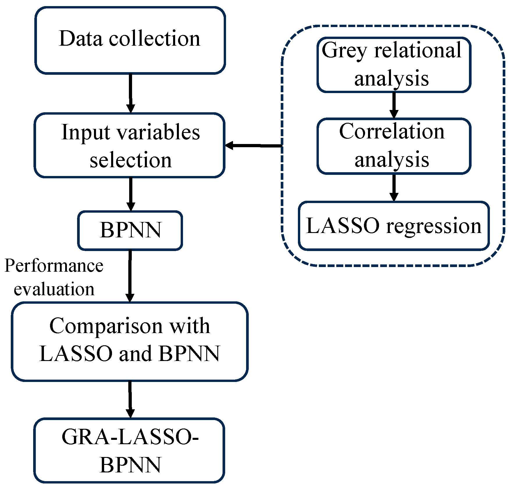
This section describes the architecture of the GRA-LASSO-BPNN hybrid prediction model and the methods used for data collection. It examines the GRA method, which identifies key drivers of residential costs; the LASSO method, which further refines input variables through regularization; and the BPNN, which possesses strong learning capabilities and robustness. The establishment process of the GRA-LASSO-BPNN hybrid prediction model is shown in Figure 1.

Figure 1.
The flowchart of GRA-LASSO-BPNN.
2.1. Data Collection Method
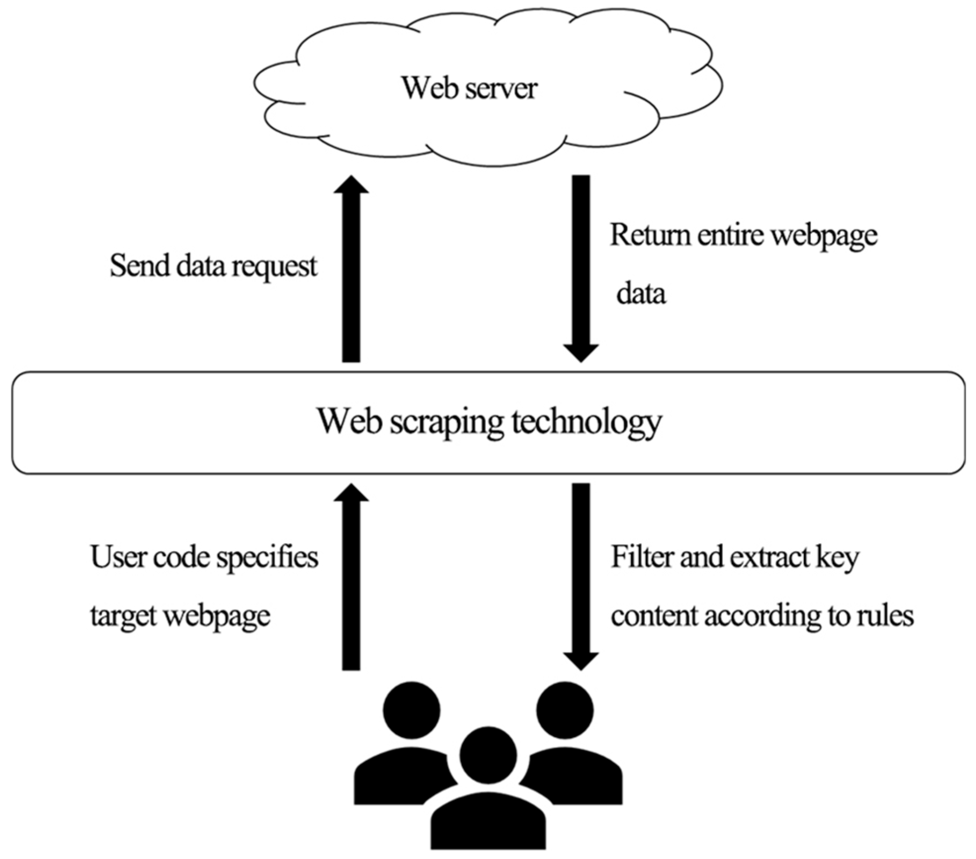
Residential project data are considered confidential by companies, making it difficult for individuals to access them. Therefore, this paper primarily uses web scraping technology [30] and writing programmes to download data from cost information websites and extract key data from web pages according to certain rules to obtain residential construction project data. The main workflow is shown in Figure 2. This section mainly implements the following three functions:
- Data Request: Send a request to the server of the specified website to obtain its corresponding web content.
- Webpage Analysis: Use regular expressions and other rules to selectively filter the needed information from the extensive content on the web server.
- Data Storage: Save the initially captured key information into files in formats such as EXCEL to prepare for subsequent data preprocessing.
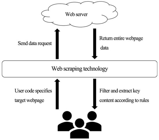
Figure 2.
Main workflow of web scraping technology [30].
Figure 2.
Main workflow of web scraping technology [30].
2.2. Grey Relational Analysis
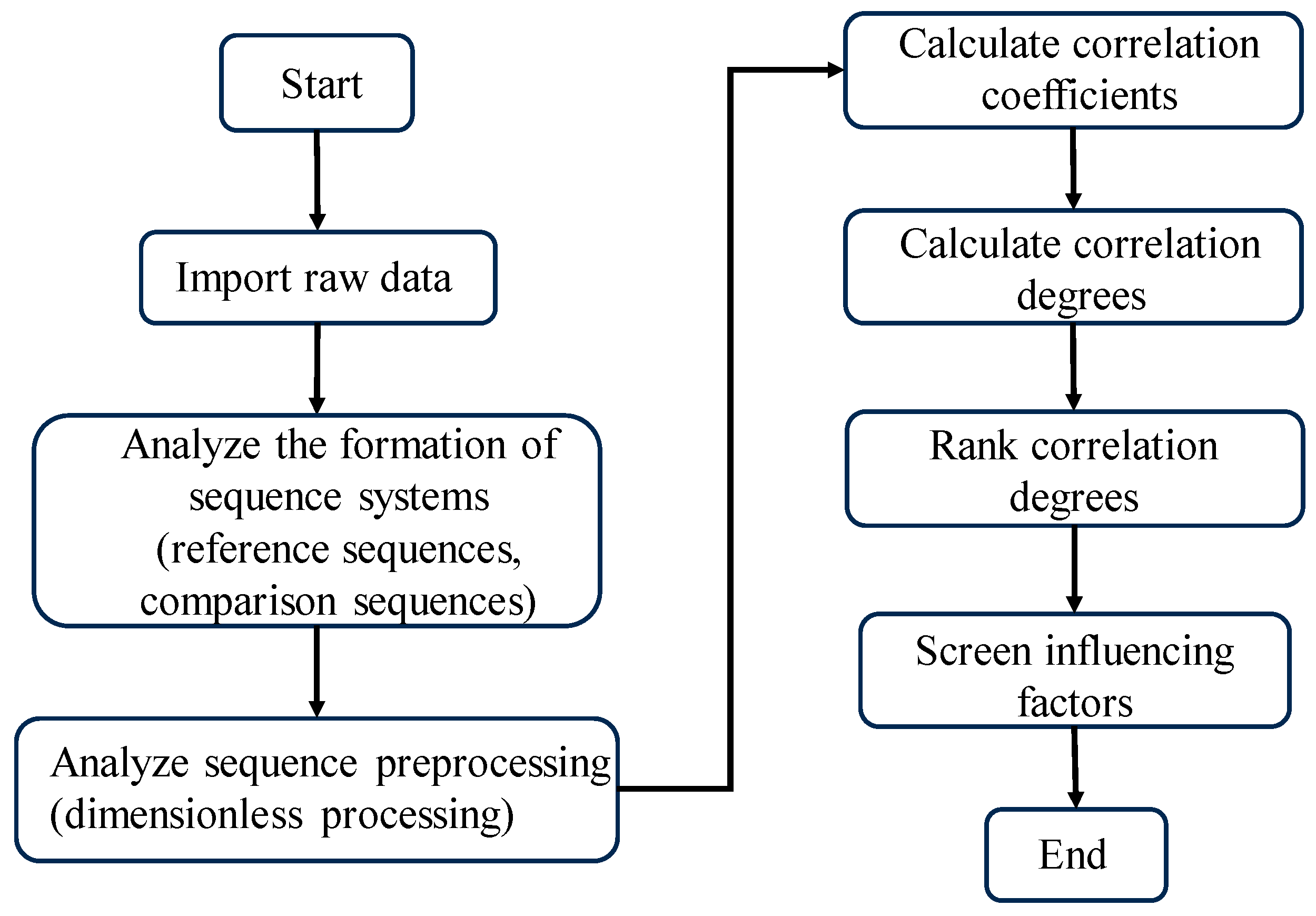
The calculation of the relational degree between engineering cost indicators is crucial for predicting residential unit costs. GRA uses grey relational degrees to measure the order of strength between factors. It is a method based on samples to evaluate the relationships between factors [31]. This method determines whether the data series curves are closely related by comparing their trends. If the sample data series reflect a consistent trend of changes between two factors, their relational degree is relatively high; otherwise, it is low. As shown in Figure 3, this method quantitatively analyzes the development trend of the dynamic process and compares the geometric relationship of the relevant statistical sequence data to calculate the grey relational degree. The calculation steps of GRA are as follows:
Step 1—Determine the Analysis Sequence: This is similar to determining the dependent variable Y and the independent variable X, identifying the system’s reference sequence and the comparative sequence.
Step 2—Normalize the Sequence Data: To obtain accurate comparison results and simplify calculations, the data must be standardized to eliminate the effects of different dimensions in the data series.
Step 3: Calculate the Relational Coefficient:
where |x0(k) − xi(k)| represents the absolute value of the difference between each data point and the reference sequence data. ρ is the distinguishing coefficient, which is usually set to 0.5 to increase the differences and stability of the correlation coefficients [32].
Step 4—Calculate the Relational Degree: Since the relational coefficients are scattered and not easy to compare as a whole, Equation (4) is used to calculate the grey relational degree.
The larger the value of αi, the higher the correlation degree, indicating a closer relationship and development trend.
Step 5—Rank the Strength of Grey Relational Degrees: Sort the relational degrees to show the strength of the relationship between each independent variable and the dependent variable.
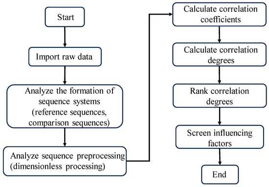
Figure 3.
Implementation principle flowchart of grey relational analysis [28].
Figure 3.
Implementation principle flowchart of grey relational analysis [28].
2.3. LASSO Regression
LASSO regression refers to adding an L1 regularization term to the minimization of the sum of squared residuals [33], as shown in Equation (5):
where denotes the L1 norm of the model coefficients, yi is the actual value, and and λ are the regularization parameter that controls the influence of the regularization term. By adjusting the value of λ, a balance can be achieved between the model’s predictive performance and feature selection.
LASSO regression can perform both variable selection and complexity adjustment, making it suitable for various types of target dependent variables, including continuous, binary, and multinomial discrete types. Through variable selection, LASSO regression can identify the most relevant independent variables from all possible ones and ignore those that are unimportant, thereby enhancing predictive performance.
2.4. GRA-LASSO-BPNN
This paper proposes a novel GRA-LASSO-BPNN cost prediction model, which is a composite prediction model based on the existing GRA, LASSO, and BPNN methods. The main steps involve data cleaning, variable selection, and finally inputting the processed data into the BPNN for training. The variable selection process combines GRA and LASSO to select variables that are strongly correlated with the unit cost of residential projects. Specifically, the GRA method is used to rank the importance of input variables, and an initial selection of variables is made using a threshold, as shown in Equations (1)–(4). This is followed by the final variable selection using LASSO regularization, as shown in Equation (5). The finalized input variables are then used as inputs for the BPNN, with the unit cost of residential projects as the output. The dataset is split into training and testing sets in a 7:3 ratio using the train–split–test approach. Finally, the performance of the GRA-LASSO-BPNN model is evaluated using model evaluation metrics to improve the accuracy of the prediction model.
2.5. Performance Evaluation
To evaluate the performance of the unit cost prediction model for residential projects, the model’s prediction accuracy is quantified using several metrics, including Mean Absolute Error (MAE), Mean Absolute Percentage Error (MAPE), Root Mean Square Error (RMSE), the coefficient of determination (R2), and Mallows’ CP value (CP). Performance evaluation metrics are shown in Equations (6)–(10). By utilizing these five different performance indicators, the prediction performance of the machine learning model can be better described. The closer the values of MAE, MSE, RMSE, and MAPE are to 0, the smaller the prediction error. Similarly, the closer the R2 value is to 1, the smaller the error.
Here, n represents the number of samples, represents the true value of the i-th sample, represents the predicted value of the i-th sample, and represents the mean of the true values.
Mallows’ CP value, proposed by statistician Colin Mallows, is an indicator that considers both model complexity and prediction accuracy, and it is used for selecting linear regression models.
where n is the number of samples, MSEall is the mean squared error of the model containing all feature variables, MSEp is the mean squared error of the model with the selected p feature variables, SST is the total sum of squares, and SSE is the sum of squared errors. Generally, the smaller the CP value, the better the predictive accuracy of the model, and when the Mallows’ CP index value approaches p + 1, the model bias is lower.
3. Research Applications
3.1. Data Acquisition and Preprocessing
Using data scraping technology and research by domestic and foreign scholars on factors influencing residential construction cost predictions, a dataset was preliminarily determined [34,35,36]. This dataset includes 47 residential construction projects in Shanghai, comprising 1 output variable, ‘unit cost’, and 17 input variables, as shown in Table 1. To facilitate the model’s processing and calculation of sample data, the preliminary data obtained were quantified, and normalized using min–max normalization. Min–max normalization is shown in Equation (12):

Table 1.
Relevant input variables for residential project unit cost estimation.
In this equation, x′ represents the value after min–max normalization, x is the original data value, and xmax and xmin are the specified maximum and minimum values for each indicator, respectively.
3.2. Selection of Input Variables for Residential Project Costs
3.2.1. Input Variable Importance Ranking
In this study, using the GRA, 17 input variables such as ‘project location’ and ‘structural type’ from 47 engineering projects were used as comparative sequences, and ‘unit cost’ was used as the system’s reference sequence for the grey relational analysis. The grey relational degrees between each input variable and the unit cost were calculated and sorted in descending order, resulting in the grey relational analysis outcomes shown in Table 2.
Table 2.
Results of grey relational analysis.
Typically, grey relational degree values range between [0, 1], with larger values indicating a higher similarity between two sequences. However, there is no fixed standard for the threshold of low grey relational degrees, as the required range of relational degree values varies across different application fields and specific issues [37,38,39]. Generally, different scholars may select different grey relational degree thresholds based on their experiments and experiences. Nevertheless, the specific threshold choice needs to be adjusted according to the particular problem and data circumstances and validated through experimentation for effectiveness.
Combining the research results of domestic and international scholars with the relatively small sample size of the data in this paper, to maximize data utilization, a grey relational degree threshold of 0.72 was adopted in this study. Factors with values below this threshold are considered to have a weak correlation with the target variable and are not taken into account. Thus, from the correlation ranking results in Table 2, factors X6, X2, and X7 are weakly correlated with cost changes and are considered for removal from the model. Additionally, in the relational coefficient ranking results, the importance of variables such as the total building area, eaves’ height, structural type, and number of floors aligns with conclusions from reference [40], indicating a certain degree of credibility. Therefore, the next step is to further investigate the actual predictive effectiveness of the 14 input variables selected by GRA for the residential unit cost prediction model and verify the accuracy of this selection.
3.2.2. Correlation Analysis
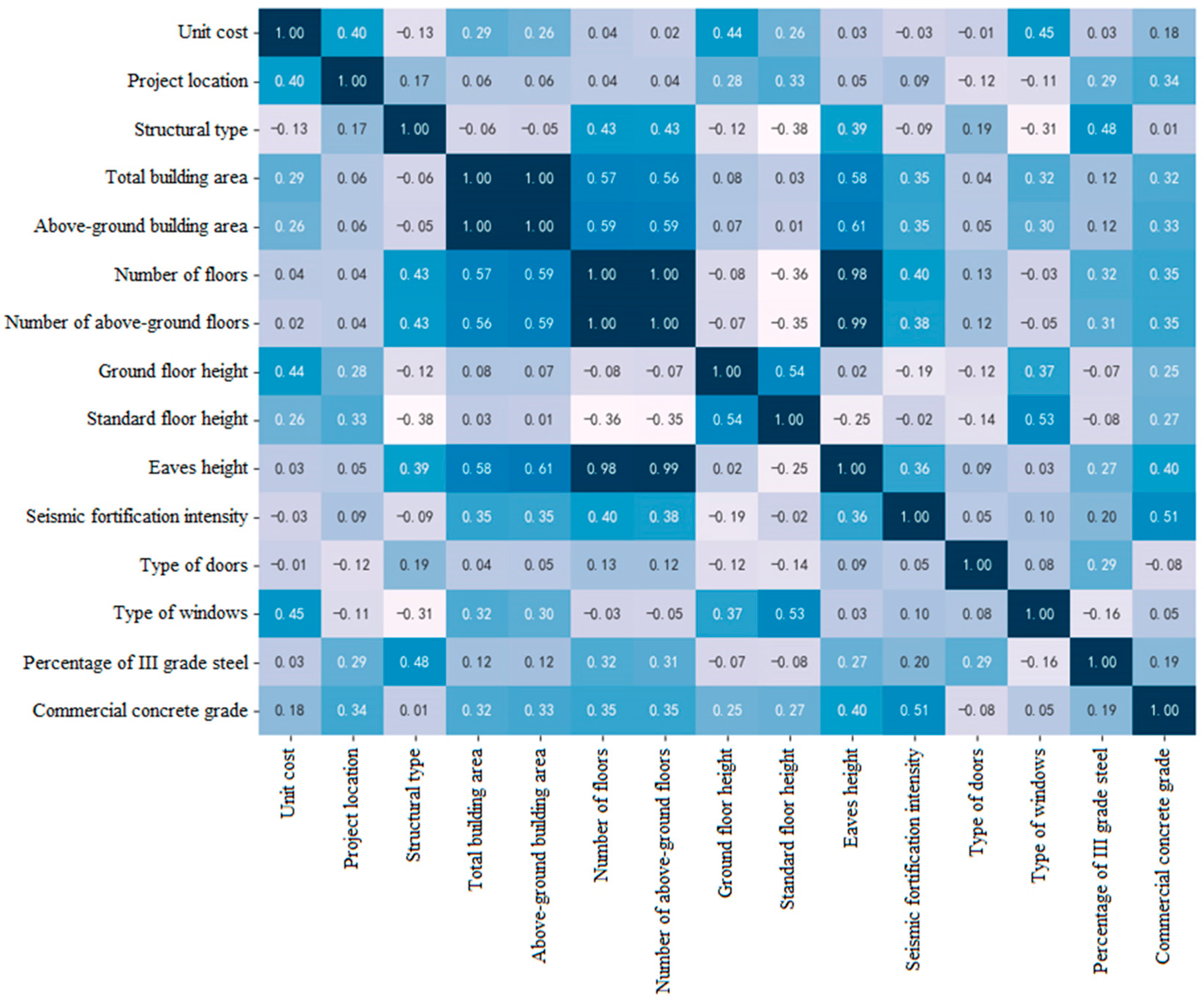
Using the sns. heatmap function package in Python3.7, after the preliminary selection of indicators by GRA, a Pearson correlation test was conducted to analyze the linear correlation between pairs of variables. The Pearson correlation coefficient ranges from [–1, 1]. The closer the absolute value is to 1, the deeper the colour, indicating a stronger linear correlation between the two variables.
As shown in Figure 4, high correlation degrees are observed between eaves’ height (X12) and the number of floors (X8), and above-ground building area (X5), with coefficients of 0.98 and 0.61, respectively. The number of floors (X8) also shows correlation with seismic fortification intensity (X13) and above-ground building area (X5), with coefficients of 0.40 and 0.59, respectively. Furthermore, seismic fortification intensity (X13) and commercial concrete grade (X17) have a correlation coefficient of 0.51, among others. Generally, the more floors a building has, the higher the eaves’ height and the larger the building area. Regarding the relationship between seismic fortification intensity and the number of floors and commercial concrete grade, multi-storey buildings require higher seismic fortification intensity than single-storey buildings, and higher seismic fortification intensity demands higher commercial concrete grades to ensure stable seismic performance. Therefore, these correlation results meet the requirements and are considered credible. The total building area (X4) and above-ground building area (X5) have a linear correlation coefficient of 1.0, indicating an extremely high correlation. In econometrics, it is usually considered that if the Pearson coefficient is greater than 0.7, there is multicollinearity between the two variables [41]. This means that the change in one variable will affect other independently related variables, a common issue in multiple regression analyses. This multicollinearity can affect the predictive accuracy of the regression model. The LASSO regression prediction method can effectively solve this problem. Therefore, based on the initial variable selection by GRA, the LASSO method will be further used to select input variables. The 47 residential construction project datasets will be randomly divided into 33 training samples and 14 test samples in a 7:3 ratio to construct a regression prediction model using a hybrid model approach.
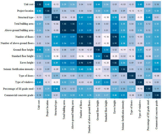
Figure 4.
Pearson correlation analysis results.
3.2.3. Determination of Input Variables
This study sets the penalty coefficient Alpha of LASSO regression to control the intensity of the first-order penalty function (L1) regularization. The larger the penalty coefficient, the stronger the constraint on fitting models with more variables, causing the regression coefficients of less influential variables to decay to zero. This results in retaining only important features, thus obtaining a GRA-LASSO regression model with better performance parameters.
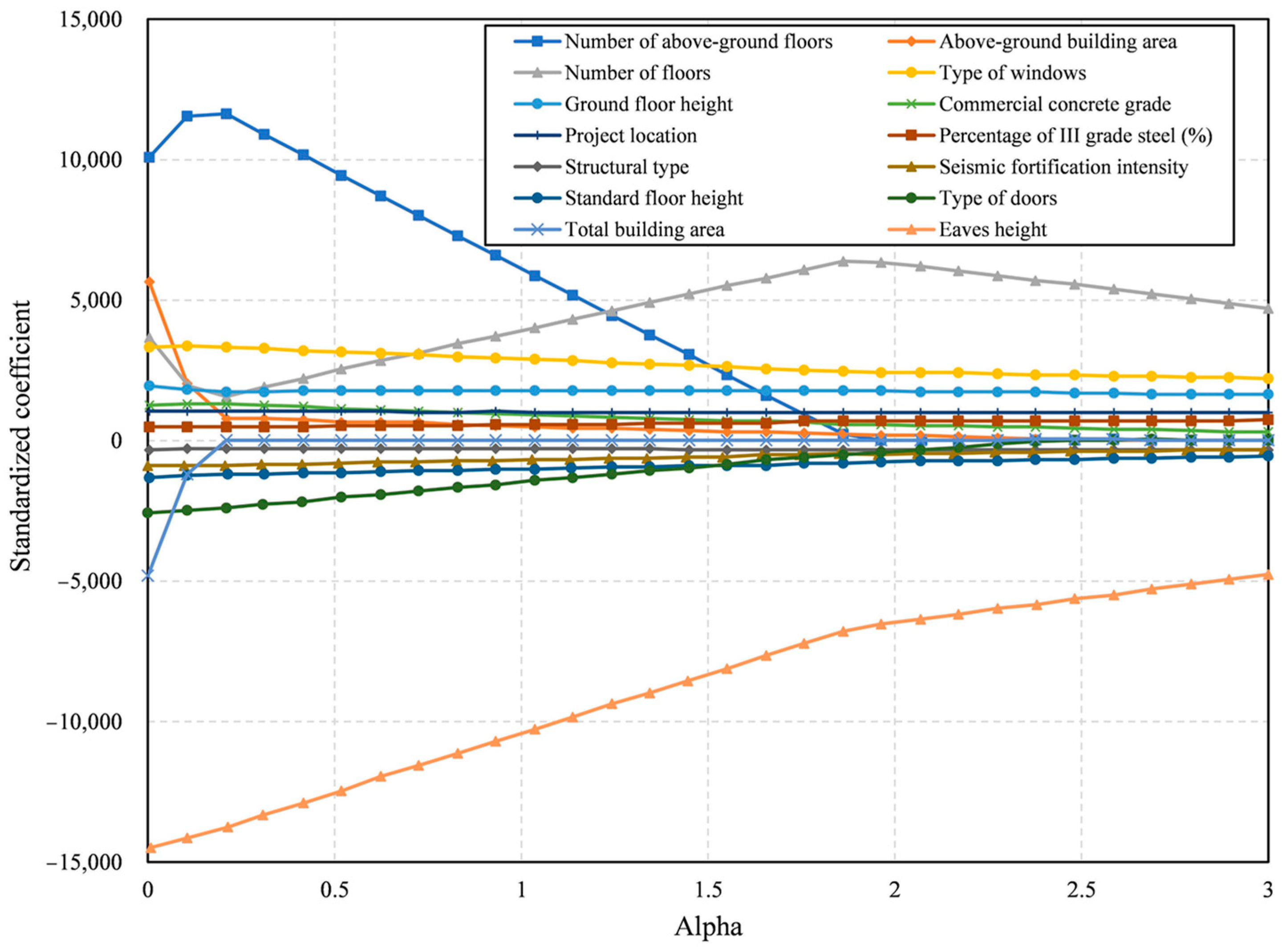
Figure 5 shows the variable coefficient trajectory of the GRA-LASSO, illustrating how the coefficients of independent variables change with the Alpha parameter. The horizontal axis represents the penalty coefficient Alpha, ranging from [0, 3], and the vertical axis represents the size of the regression coefficients of the variables. Figure 5 intuitively shows the changes in the coefficients of the 14 different input variables preliminarily selected by GRA and which independent variable coefficients are compressed to zero first under different Alpha parameters.
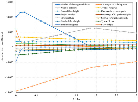
Figure 5.
LASSO variable regression coefficient path solution.
As seen in Figure 5, as the Alpha value increases, the regularization intensity increases, and the coefficients of the 14 variables are gradually compressed to zero. The coefficients of total building area and the number of above-ground floors decay to zero the fastest, indicating that these independent variables are the first to be filtered out in the model. This also validates the correctness of the Pearson correlation analysis.
But the performance of the LASSO regression model varies with different numbers of variables. Therefore, this study uses the MAPE, the coefficient of determination R2, and the statistical Mallows’ CP value to measure the goodness of fit of the model.
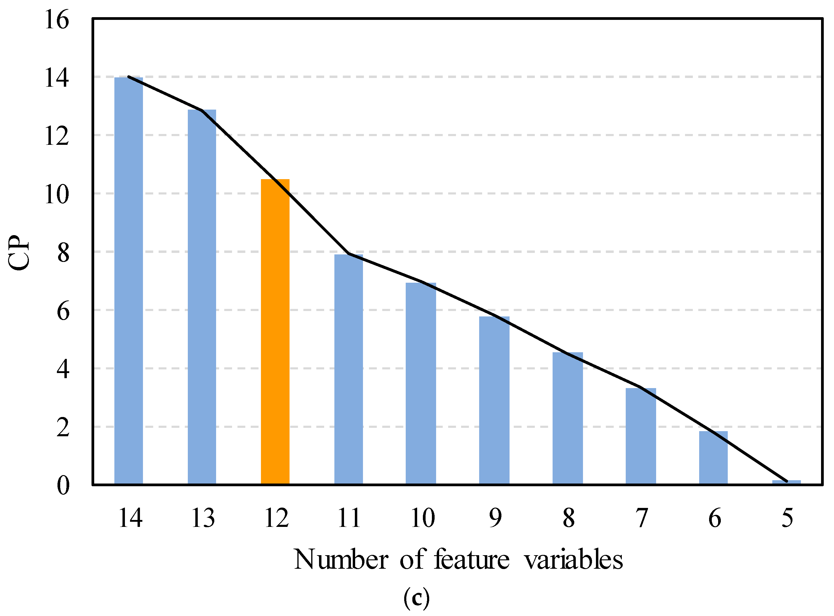
Figure 6 shows the fluctuations of these indicators in the GRA-LASSO model with the number of feature variables. According to the results, the model with 12 feature variables is considered the optimal model. This model has the lowest MAPE and the highest R2, while also meeting the requirement of the unbiased model with Mallows’ CP index close to the number of feature variables + 1, indicating low bias in the model. At this point, combining the GRA-LASSO variable selection where the regression coefficients of the number of above-ground floors and the total building area were first compressed to zero, the remaining 12 variables are determined as the input features for the BPNN model.
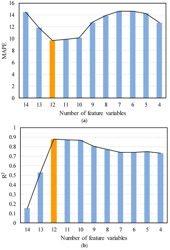

Figure 6.
Model performance metrics with varying numbers of independent variables. (a) MAPE, (b) R2, (c) CP.
3.3. GRA-LASSO-BP Prediction Model Establishment
The 12 influencing factors selected by LASSO regression—the seismic fortification intensity, commercial concrete grade, type of windows, type of doors, standard floor height, ground floor height, percentage of grade III steel, above-ground building area, eaves’ height, structural type, number of floors, and region—are used as input variables. The unit cost is used as the output variable, and then the BPNN model is used for prediction. Where the number of variables in the BPNN input layer is 12, the number of variables in the output layer is 1 and the number of hidden layers is 14. The learning rate was set at 0.01, with 300 iterations, and the loss function used was MSE.
4. Results and Discussion
4.1. Conclusion and Analysis of Input Variable Selection
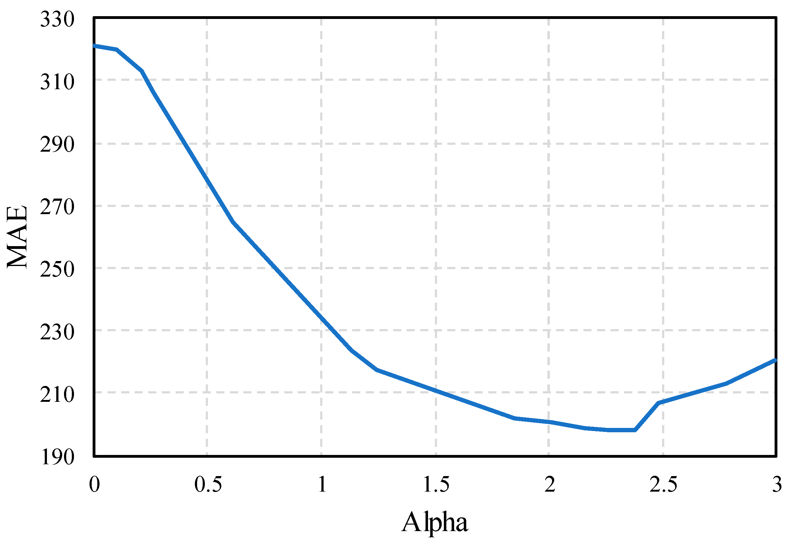
The importance of the input variables affecting the unit cost of residential projects was ranked using GRA. Through a preliminary screening based on threshold values, three variables with less impact—the underground building area, number of underground floors, and presence of a basement—were filtered out. However, the further selection of input variables required regularization through LASSO regression. After LASSO regularization, the input variables were reduced to 14, as shown in Figure 7.

Figure 7.
Mean Absolute Error as Alpha varies.
Although some variable coefficients may initially show an upward trend, the overall trend is that the variable coefficients approach zero. As the regularization intensity increases, less influential variables are eventually eliminated, retaining only important variables. The model increasingly tends towards a simpler form during this process. However, a simpler model is not always better. As shown in Figure 7, the Mean Absolute Error (MAE) of the regression prediction model initially decreases and then increases as Alpha gradually increases. Therefore, selecting an appropriate Alpha value in practical applications is necessary to achieve a GRA-LASSO prediction model with better performance parameters.
Even though GRA and LASSO regularization have reduced the input variables to 14, the performance of the GRA-LASSO regression model varies with different numbers of variables. Therefore, the model performance was tested with different numbers of variables, eventually leading to the selection of 12 input variables. These were then input into the BPNN for training.
4.2. Performance Analysis of the Residential Project Cost Estimation Hybrid Model
To verify the performance of the GRA-LASSO-BPNN prediction model proposed in this paper, its prediction results were compared with those obtained using the BPNN and LASSO regression methods alone, as well as with the actual unit costs. The LASSO regression model is specifically shown in Equation (13). The BPNN method and its specific parameters are detailed in Section 3.3.
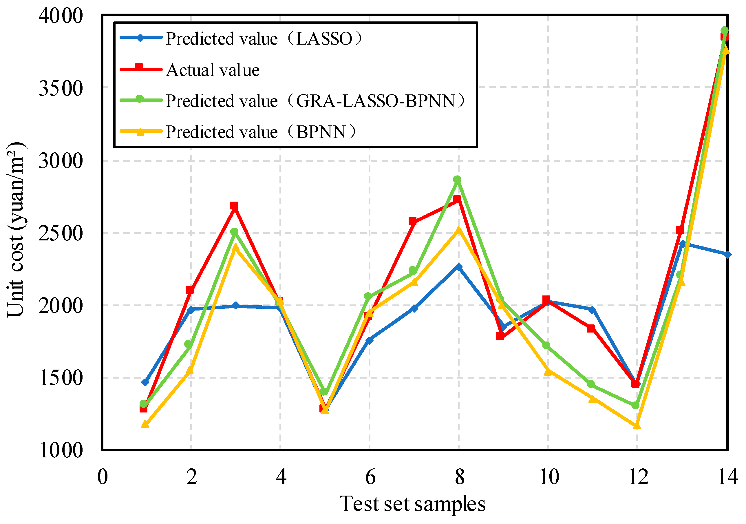
The prediction results of the three methods on the test set, compared to the actual values, are shown in Figure 8. These prediction results were quantitatively analyzed using evaluation metrics such as MAE, MSE, and RMSE. The calculation methods for MAE, MSE, and RMSE are shown in Equations (6)–(8), respectively. The results are presented in Table 3.
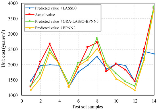
Figure 8.
Visual comparison of performance of three predictive models on test set.
Table 3.
Comparison of evaluation metrics for each model.
As shown in Figure 8, the predicted values of the GRA-LASSO-BPNN regression model are generally consistent with the trend of the actual costs, with relatively small errors. Table 3 indicates that the MAE of the GRA-LASSO-BPNN model is 197.02, the RMSE is 234.64, and the MSE is 55,057.04. The errors of these three evaluation metrics are all smaller than those of the BPNN and LASSO regression methods used alone, and the MAE of GRA-LASSO-BPNN is 29% lower than that of LASSO with the largest error, and 20% less than that of the BPNN model without screening for input variables. Therefore, the prediction performance of GRA-LASSO-BPNN is the best.
5. Conclusions
This study utilized GRA, Pearson correlation coefficients, and LASSO regression regularization to select input variables and establish the GRA-LASSO-BPNN hybrid prediction model. This model is designed to assist cost estimation personnel in real estate companies in making more reasonable, accurate, and efficient cost estimates for residential construction projects during the early stages of investment decision-making, thereby significantly reducing project costs. The main findings include the following:
- Among the 17 input variables, the ones with the most significant impact on the unit cost of residential projects in Shanghai, after GRA and LASSO regularization, are the seismic fortification intensity, commercial concrete grade, type of doors and windows, and total building area. A total of 12 input variables were ultimately selected.
- The evaluation metrics of the proposed GRA-LASSO-BPNN hybrid prediction model are significantly lower than those of the BPNN and LASSO regression models, indicating that the GRA-LASSO-BPNN hybrid prediction model proposed in this study has superior predictive performance in estimating residential project costs.
- The GRA-LASSO-BPNN model outperforms the BPNN model alone, demonstrating that input variable selection can enhance model prediction accuracy. Additionally, when comparing the BPNN and LASSO models, as well as the GRA-LASSO-BPNN and LASSO models, it is evident that the errors of the hybrid models are lower than those of LASSO, suggesting that BPNN can improve prediction accuracy on high-dimensional small sample datasets.
The proposed early-stage cost estimation model for residential project investment decision-making is currently applicable only to the Shanghai region. However, if the dataset becomes sufficiently large, it could be widely applied to cost estimation for residential projects across the country. Future work aims to achieve the following goals:
- Collect more datasets to further reduce prediction model errors.
- Introduce additional relevant feature parameters that impact the cost of underground structures, and then use GRA-LASSO for feature selection.
- Introduce optimization algorithms to improve the GRA-LASSO-BPNN model.With the progressive informatization of construction, deep learning is expected to become increasingly integral to the cost management in construction.
Author Contributions
Conceptualization, L.C. and D.W.; methodology, L.C.; software, D.W.; validation, L.C.; formal analysis, L.C.; investigation, L.C.; resources, D.W.; data curation, L.C.; writing—original draft preparation, L.C.; writing—review and editing, D.W.; visualization, L.C.; supervision, D.W. All authors have read and agreed to the published version of the manuscript.
Funding
This research received no external funding.
Data Availability Statement
The data used in this research can be found via the corresponding author.
Conflicts of Interest
The authors declare that they have no conflicts of interest.
References
- Dandan, T.H.; Sweis, G.; Sukkare, L.S.; Sweis, R.J. Factors affecting the accuracy of cost estimate during various design stages. J. Eng. Des. Technol. 2019, 18, 787–819. [Google Scholar] [CrossRef]
- Wang, B.; Dai, J. Discussion on the prediction of engineering cost based on improved BP neural network algorithm. J. Intell. Fuzzy Syst. 2019, 37, 6091–6098. [Google Scholar] [CrossRef]
- Stoy, C.; Kalusche, W. The determination of occupancy costs during early project phases. Constr. Manag. Econ. 2006, 24, 933–944. [Google Scholar] [CrossRef]
- Bimenyimana, S.; Asemota, G.N.O.; Ihirwe, P.J.; Mesa, K.C. Performance estimation of Ntaruka hydropower plant and its comparison with the prediction results obtained by SPSS. Energy Environ. 2018, 29, 1004–1021. [Google Scholar] [CrossRef]
- Wang, Y.R.; Yu, C.Y.; Chan, H.H. Predicting construction cost and schedule success using artificial neural networks ensemble and support vector machines classification models. Int. J. Proj. Manag. 2012, 30, 470–478. [Google Scholar] [CrossRef]
- Jin, R.Z.; Cho, K.M.; Hyun, C.T.; Son, M.J. MRA-based revised CBR model for cost prediction in the early stage of construction projects. Expert Syst. Appl. 2012, 39, 5214–5222. [Google Scholar] [CrossRef]
- Son, H.; Kim, C.; Kim, C. Hybrid principal component analysis and support vector machine model for predicting the cost performance of commercial building projects using pre-project planning variables. Autom. Constr. 2012, 27, 60–66. [Google Scholar] [CrossRef]
- Ongpeng, J.; Roxas, C. An artificial neural network approach to structural cost estimation of building projects in the Philippines. In Proceedings of the DLSU Research Congress, Manila, Philippines, 6–8 March 2014. [Google Scholar]
- Bala, K.; Bustani, S.A.; Waziri, B.S. A computer-based cost prediction model for institutional building projects in Nigeria: An artificial neural network approach. J. Eng. Des. Technol. 2014, 12, 519–530. [Google Scholar] [CrossRef]
- Deepa, G.; Niranjana, A.J.; Balu, A.S. A hybrid machine learning approach for early cost estimation of pile foundations. J. Eng. Des. Technol. 2023; ahead-of-print. [Google Scholar] [CrossRef]
- Ye, D. An Algorithm for Construction Project Cost Forecast Based on Particle Swarm Optimization-Guided BP Neural Network. Sci. Program. 2021, 2021, 8. [Google Scholar] [CrossRef]
- Du, Z.; Li, B. Construction project cost estimation based on improved BP neural network. In Proceedings of the 2017 International Conference on Smart Grid and Electrical Automation (ICSGEA), Changsha, China, 27–28 May 2017. [Google Scholar]
- Feng, G.L.; Li, L. Application of genetic algorithm and neural network in construction cost estimate. Adv. Mat. Res. 2013, 756–759, 3194–3198. [Google Scholar] [CrossRef]
- Sandoval-Moreno, G.; Galea, M.; Arellano-Valle, R. Inference in multivariate regression models with measurement errors. J. Stat. Comput. Simul. 2023, 93, 1997–2025. [Google Scholar] [CrossRef]
- De Mello, R.; Manapragada, C.; Bifet, A. Measuring the Shattering coefficient of Decision Tree models. Expert Syst. Appl. 2019, 137, 443–452. [Google Scholar] [CrossRef]
- Sabzekar, M.; Hasheminejad, S.M.H. Robust regression using support vector regressions. Chaos Solitons Fractals 2021, 144, 110738. [Google Scholar] [CrossRef]
- Wang, S.Z.; Ji, B.X.; Zhao, J.S.; Liu, W.; Xu, T. Predicting ship fuel consumption based on LASSO regression. Transport. Res. Part D—Transp. Environ. 2018, 65, 817–824. [Google Scholar] [CrossRef]
- Li, Z.T.; Jiang, L.L.; Zhao, R.; Huang, J.; Yang, W.; Wen, Z.; Zhang, B.; Du, G. MiRNA-based model for predicting the TMB level in colon adenocarcinoma based on a LASSO logistic regression method. Medicine 2021, 100, e26068. [Google Scholar] [CrossRef]
- Lee, J.H.; Shi, Z.T.; Gao, Z. On LASSO for predictive regression. J. Econom. 2022, 229, 322–349. [Google Scholar] [CrossRef]
- Meharie, M.G.; Gariy, Z.; Mutuku, R.; Mengesha, W.J. An effective approach to input variable selection for preliminary cost estimation of construction projects. Adv. Civ. Eng. 2019, 2019, 1–14. [Google Scholar] [CrossRef]
- Alshemosi, A.M.B.; Alsaad, H.S.H. Cost estimation process for construction residential projects by using multifactor linear regression technique. Int. J. Sci. Res. 2017, 6, 151–156. [Google Scholar]
- Greenacre, M.; Groenen, P.J.F.; Hastie, T.; D’Enza, A.I.; Markos, A.; Tuzhilina, E. Principal component analysis. Nat. Rev. Methods Primers 2022, 2, 100. [Google Scholar] [CrossRef]
- Sayed, M.; Abdel-Hamid, M.; El-Dash, K. Improving cost estimation in construction projects. Int. J. Constr. Manag. 2020, 23, 135–143. [Google Scholar] [CrossRef]
- Youssefi, I.; Celik, T. Optimized approach toward identification of influential cost overrun causes in construction industry. ASCE-ASME J. Risk Uncertain. Eng. Syst. Part A Civ. Eng. 2023, 9, 04023003. [Google Scholar] [CrossRef]
- Mao, S.; Tseng, C.H.; Shang, J.; Wu, Y.; Zeng, X.J. In Proceedings of Construction cost index prediction: A visibility graph network method. In Proceedings of the 2021 International Joint Conference on Neural Networks (IJCNN), Shenzhen, China, 18–22 July 2021. [Google Scholar]
- Wang, C.X.; Qiao, J.L. Construction Project Cost Prediction Method Based on Improved BiLSTM. Appl. Sci. 2024, 14, 978. [Google Scholar] [CrossRef]
- Gai, R.; Guo, Z. A Water Quality Assessment Method Based on an Improved Grey Relational Analysis and Particle Swarm Optimization Multi-classification Support Vector Machine. Front. Plant Sci. 2023, 14, 1099668. [Google Scholar] [CrossRef] [PubMed]
- Tong, B.; Guo, J.J.; Fan, S. Predicting Budgetary Estimate of Highway Construction Projects in China Based on GRA-LASSO. J. Manage. Eng. 2021, 37, 04021012. [Google Scholar] [CrossRef]
- Yu, W.K.; Wu, H.R.; Peng, C. Short-Term Price Forecast of Vegetables Based on Combination Model of Lasso Regression Method and BP Neural Network. Smart Agric. 2020, 2, 108–117. [Google Scholar]
- Muehlethaler, C.; Albert, R. Collecting data on textiles from the internet using web crawling and web scraping tools. Forensic Sci. Int. 2021, 322, 110753. [Google Scholar] [CrossRef]
- Shi, T.; Jiang, W.; Luo, P. A Method of Clustering Ensemble Based on Grey Relation Analysis. Wirel. Pers. Commun. 2018, 103, 871–885. [Google Scholar] [CrossRef]
- Singh, T.; Patnaik, A.; Chauhan, R. Optimization of tribological properties of cement kiln dust-filled brake pad using grey relation analysis. Mater. Des. 2016, 89, 1335–1342. [Google Scholar] [CrossRef]
- Tibshirani, R. Regression shrinkage and selection via the lasso. J. R. Stat. Soc. Ser. B 1996, 58, 267–288. [Google Scholar] [CrossRef]
- Fang, S.; Zhao, T.; Zhang, Y. Prediction of construction projects’ costs based on fusion method. Eng. Comput. 2017, 34, 2396–2408. [Google Scholar]
- Rafiei, M.H.; Adeli, H. Novel machine-learning model for estimating construction costs considering economic variables and indexes. J. Constr. Eng. Manag. 2018, 144, 04018106. [Google Scholar] [CrossRef]
- Ahn, J.; Park, M.; Lee, H.S.; Ahn, S.J.; Ji, S.H.; Song, K.; Son, B.S. Covariance effect analysis of similarity measurement methods for early construction cost estimation using case-based reasoning. Autom. Constr. 2017, 81, 254–266. [Google Scholar] [CrossRef]
- Jiang, S.J. Green supplier selection for sustainable development of the automotive industry using grey decision-making. Sustain. Dev. 2018, 26, 890–903. [Google Scholar] [CrossRef]
- Zeng, B.; Guo, J.; Zhang, F.; Zhu, W.; Xiao, Z.; Huang, S.; Fan, P. Prediction model for dissolved gas concentration in transformer oil based on modified grey wolf optimizer and LSSVM with grey relational analysis and empirical mode decomposition. Energies 2020, 13, 422. [Google Scholar] [CrossRef]
- Delcea, C.; Cotfas, L.A. Public opinion assessment through grey relational analysis approach. In Advancements of Grey Systems Theory in Economics and Social Sciences; Springer Nature: Singapore, 2023; pp. 179–199. [Google Scholar]
- Fan, H.B. Research on Estimation Model of Construction Cost Based on Optimal Neural Network. Master’s Dissertation, Shenyang Jianzhu University, Shenyang, China, 2019. [Google Scholar]
- Wang, D.H. Multivariate Statistical Analysis and SPSS Applications; East China University of Science and Technology Press: Shanghai, China, 2010. [Google Scholar]

Disclaimer/Publisher’s Note: The statements, opinions and data contained in all publications are solely those of the individual author(s) and contributor(s) and not of MDPI and/or the editor(s). MDPI and/or the editor(s) disclaim responsibility for any injury to people or property resulting from any ideas, methods, instructions or products referred to in the content. |
© 2024 by the authors. Licensee MDPI, Basel, Switzerland. This article is an open access article distributed under the terms and conditions of the Creative Commons Attribution (CC BY) license (https://creativecommons.org/licenses/by/4.0/).