Advancements in Deep Learning Techniques for Time Series Forecasting in Maritime Applications: A Comprehensive Review

Abstract

The maritime industry is integral to global trade and heavily depends on precise forecasting to maintain efficiency, safety, and economic sustainability. Adopting deep learning for predictive analysis has markedly improved operational accuracy, cost efficiency, and decision-making. This technology facilitates advanced time series analysis, vital for optimizing maritime operations. This paper reviews deep learning applications in time series analysis within the maritime industry, focusing on three areas: ship operation-related, port operation-related, and shipping market-related topics. It provides a detailed overview of the existing literature on applications such as ship trajectory prediction, ship fuel consumption prediction, port throughput prediction, and shipping market prediction. The paper comprehensively examines the primary deep learning architectures used for time series forecasting in the maritime industry, categorizing them into four principal types. It systematically analyzes the advantages of deep learning architectures across different application scenarios and explores methodologies for selecting models based on specific requirements. Additionally, it analyzes data sources from the existing literature and suggests future research directions.

1. Introduction

The maritime industry is navigating a complex environment, grappling with increasingly stringent trade policies, heightened geopolitical tensions, and evolving globalization patterns [1]. Adding to these difficulties and challenges, the climate is intricate and the volume of sea traffic is immense, further straining the industry [2]. Nevertheless, maritime trade remains the cornerstone of global commerce, driving economic growth and underpinning the global economy [3,4]. Amid these complexities, the rapid development of satellite communications, large-scale wireless networks, and data science technologies has revolutionized the shipping industry. These advancements have made the comprehensive tracking of global ship movements and trends feasible [5]. The richness and diversity of collected maritime data have significantly enhanced the accuracy and effectiveness of maritime applications, making them indispensable in modern maritime operations [6,7,8]. Deep learning technologies for time series forecasting in maritime applications have garnered significant interest, particularly in facing these challenges. These technologies offer promising solutions, helping the maritime industry manage safety, optimize operations, and address future challenges more effectively.

However, there are several notable gaps in the existing literature. Existing studies primarily focus on applying and optimizing individual deep learning models, lacking systematic and comprehensive comparative analysis. For instance, different studies employ various models, datasets, and experimental setups, making it challenging to conduct effective horizontal comparisons. This hinders a complete understanding of the strengths and weaknesses of different deep learning methods in maritime time series analysis and their appropriate application scenarios. Moreover, the performance variations of different models in diverse application environments have not been thoroughly explored. While some studies indicate that certain models excel in specific tasks, these results are often based on particular datasets and experimental conditions, lacking generalizability. More comprehensive research is needed to reveal which models have advantages across various maritime applications and how to select and optimize models based on specific needs.

To overcome these research gaps, this review examines the applications of deep learning in time series analysis within the maritime industry, focusing on three key areas: ship operation-related, port operation-related, and shipping market-related topics. For the purpose of obtaining relevant literature, extensive searches were conducted in major international databases such as the Web of Science and Scopus to gather bibliometric data suitable for analysis. Our strategy used specific keywords to identify studies employing deep learning architectures for time series data in the maritime domain. After screening and removing duplicates, we collected 89 papers on these topics. Most of the collected literature, 79%, pertains to ship operations, highlighting the interest in forecasting ship operation processes using deep learning. This comprehensive data collection underscores the increasing reliance on advanced computational techniques to enhance maritime research and operations.

This review explores the diverse applications of deep learning in the maritime domain, emphasizing its role in enhancing ship operation-related tasks, port operations, and shipping market forecasting. Specifically, it delves into applications such as ship trajectory prediction, anomaly detection, intelligent navigation, and fuel consumption prediction. These applications leverage the unique advantages of deep learning models such as the Artificial Neural Network (ANN), Multilayer Perceptron (MLP), Deep Neural Network (DNN), Long Short-Term Memory (LSTM) network, Temporal Convolutional Network (TCN), Recurrent Neural Network (RNN), Gated Recurrent Unit (GRU), Convolutional Neural Network (CNN), Random Vector Functional Link (RVFL) network, and Transformer models to address specific maritime challenges. Through comparative analysis, we aim to uncover the performance and suitability of different deep learning models in various maritime applications, thereby guiding future research and practical applications. Future research directions emphasize improving data processing and feature extraction, optimizing deep learning models, and exploring specific maritime applications, including ship trajectory prediction, port forecasts, ocean environment modeling, fault diagnosis, and cross-domain applications.

The remainder of this work is organized as follows: Section 2 introduces the literature review methods. In Section 3, deep learning methods are presented. The applications of deep learning in time series forecasting within the maritime domain are discussed in Section 4. An overall analysis is provided in Section 5. Finally, Section 6 concludes the paper and outlines the limitations of the research.

2. Literature Collection Procedure

To acquire the pertinent literature, major international databases including the Web of Science and Scopus were utilized to search for bibliometric data suitable for analysis. The rationale for choosing these specific databases is that they are among the most extensive academic and scientific research repositories. These databases are widely recognized for their broad coverage of diverse disciplines. They are considered critical resources for accessing high-quality, peer-reviewed articles crucial for conducting a thorough literature review. Figure 1 is a flowchart that displays the overall process from the methods of data collection through the criteria for filtering to the final selection of references. The search strategy used for the two search engines is as follows:

• Search scope: Titles, Keywords, and Abstracts
• Keywords 1: ‘deep’ AND ‘learning’, AND
• Keywords 2: ‘time AND series’, AND
• Keywords 3: ‘maritime’, OR
• Keywords 4: ‘vessel’, OR
• Keywords 5: ‘shipping’, OR
• Keywords 6: ‘marine’, OR
• Keywords 7: ‘ship’, OR
• Keywords 8: ‘port’, OR
• Keywords 9: ‘terminal’

The primary function of the first two sets of keywords is to narrow the search scope to studies that use deep learning architectures for predicting time series data. Subsequent keywords are used to narrow the search scope, all related to the maritime domain. After conducting an initial search using the above strategy and manually removing duplicates between the two databases, 482 papers were collected. Given that the keywords used might include cases of polysemy, a second screening is necessary. The strategy for this second screening is as follows:

• Retain only articles related to maritime operations. For example, studies on ship-surrounding weather and risk prediction based on ship data will be kept, while research solely focused on marine weather or wave prediction that is unrelated to any aspect of maritime operations will be excluded.
• Exclude neural network studies that do not employ deep learning techniques, such as ANN or MLP with only one hidden layer.
• The language of the publications must be English.
• The original data used in the papers must include time series sequences.

After undergoing keyword filtering and manual screening, we retained 89 papers that utilize deep learning architectures and are based on time series data for predictions within the maritime domain.

3. Deep Learning Algorithms

3.1. Artificial Neural Network (ANN)

The ANN forms a type of machine learning model that is structured to reflect the human brain’s neural configuration, which is noted for its effective performance [9]. Structurally, a traditional ANN consists of three key layers: the input layer, one or more hidden layers, and the output layer [10]. In this setup, raw data are first gathered in the input layer and then processed through the hidden layers where patterns and features are extracted. The processed information is finally sent to the output layer, which generates the predictive outcomes. The normalization of input and output data, typically within a range of 0 to 1 or −1 to 1, ensures stability and efficiency during training by preventing numerical issues and enhancing convergence rates. The foundational architecture of the ANN shown in Figure 2 consists of three layers: an input layer comprising four neurons (I_1 to I_4), a hidden layer containing four neurons, and an output layer featuring a single neuron (E). Each neuron is interconnected through weights optimized during training, allowing the network to perform tasks such as prediction and classification effectively.

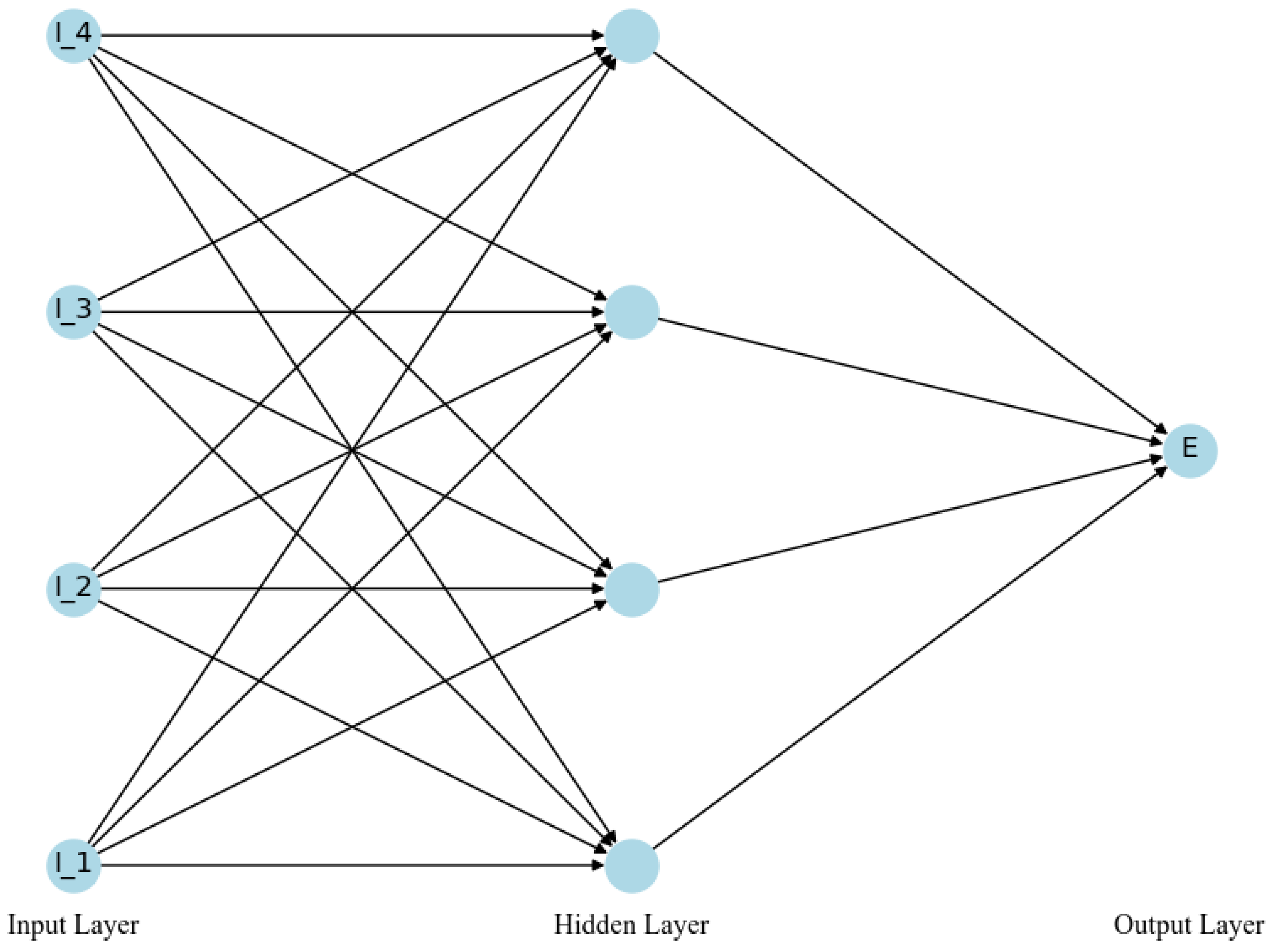
3.1.1. Multilayer Perceptron (MLP)/Deep Neural Networks (DNN)

The term ANN serves as a broad descriptor for various models, including the MLP, a fundamental archetype. The MLP’s architecture, as previously illustrated, relies on error backpropagation and gradient descent algorithms to optimize network weights [12]. These methods work together to reduce prediction errors in the model’s output [13]. Equation (1) explains the formulation of the MLP’s output.

$$y_p={\phi }_o\left\{{\sum }_{j=1}^Z{\omega }_{jp}^o\left[{\phi }_H\left({\sum }_{i=0}^Q{\omega }_{ij}^H{x}_i\right)\right]\right\}$$

(1)

where ${\omega }_{ij}^H$ signifies the weights associated with the hidden layer and ${\omega }_{jp}^o$ indicates the weights of the output layer. ${\phi }_H$ and ${\phi }_o$ symbolize the activation functions for the hidden and output layers, respectively. Commonly utilized activation functions include ReLU and Sigmoid, with the selection primarily influenced by the particular application context and the type of output required.

Conversely, the Deep Feedforward Network or Deep Neural Network (DNN), the most fundamental model in deep learning, typically features more hidden layers [14]. The increased architectural depth enhances the network’s ability to learn intricate features and patterns from the input data, thereby improving its prediction capabilities.

Within the corpus of literature compiled for this paper, two distinct studies employed the frameworks of ANN and MLP, respectively, to conduct time series forecasting. These neural network architectures were specifically utilized for predicting ship Response Amplitude Operators (RAOs) and ship classification purposes, respectively [15,16].

3.1.2. WaveNet

Recent advancements in ANN research have led to the development of high-performance models, notably the WaveNet, a generative model based on convolutional neural networks designed for audio waveform generation [17]. This model incorporates several advanced deep learning technologies, including dilated causal convolutions, residual modules, and gated activation units. The hallmark of WaveNet is its dilated convolution structure, which enables the model to effectively learn long-term dependencies within audio data, demonstrating robust learning capabilities. As a probabilistic autoregressive model, WaveNet directly learns the mappings between sequential sample values, revealing its potential across a variety of application scenarios. Figure 3 illustrates the foundational architecture of WaveNet. Furthermore, for a sequence of $x=\left\{x_1, x_2\dots , x_{t-1}\right\}$, its joint probability $p\left(x\right)$ can be represented by Equation (2). WaveNet also utilizes gated activation units, whose mathematical expression is depicted in Equation (3).

$$p\left(x\right)=\prod _{t=1}^{T}p\left(x_t \right| x_1, x_2\dots , x_{t-1})$$

(2)

$$z=\tanh \left(W_{f,k}\ast x\right)\odot \sigma (W_{g,k}\ast x)$$

(3)

where $t$ represents the time step index within the sequence; $T$ denotes the total length of the sequence; and $k$ indicates the layer index. The terms $f$ and $g$ refer to the filter and gate, respectively, while $W$ is a learnable convolution filter. A fundamental component of WaveNet is its use of causal convolutions. By employing causal convolutions, the model ensures that the temporal order of data is preserved during modeling. WaveNet enhances this approach by incorporating dilated causal convolutions. Dilated convolutions skip input values at specified intervals, allowing the convolutional kernel to cover a larger area than its actual size, which improves model performance. Figure 4 and Figure 5 illustrate causal and dilated causal convolutions, respectively. The key difference in the hidden layers is that the dilated layers in Figure 5 use different dilation rates to skip inputs. This allows the model to cover a broader range of data without increasing the number of parameters. In contrast, the hidden layers in Figure 4 process consecutive input data points, focusing on immediate information. This dilation in Figure 5 helps the model capture longer-term dependencies in the data. WaveNet has been demonstrated to be effective in synthesizing natural human speech and predicting time series [18,19].

3.1.3. Randomized Neural Network

Random neural networks, commonly used in shallow neural architectures, initialize the weights and biases of hidden layers randomly and keep them fixed during training, enhancing training efficiency [20]. This approach, integral to the construction of Extreme Learning Machines (ELMs) and the RVFL network, is particularly effective for rapid learning and streamlining model training [21,22].

ELM represents a type of random neural network, particularly emphasizing the use of a single hidden layer, where the weights and biases of the hidden layer remain fixed after initialization. Within the ELM framework, the only parameters that need optimization are the output weights, which are the weights connecting the hidden nodes to the output nodes. These are typically computed efficiently via matrix inversion operations. Figure 6 illustrates a simplified ELM architecture, and $\beta$ represents the weights associated with the connections in the network.

RVFL is an extension of ELM, retaining all core characteristics of ELM while incorporating additional direct connections from the input layer to the output layer. These direct connections include not only the weights linking hidden and output nodes but also direct linkage weights between input and output nodes. Such direct connections in RVFL networks provide additional regularization capabilities, enhancing the model’s learning capacity and generalizability [23]. In the RVFL structure, the output weights, including both direct and indirect connections, can also be computed directly through matrix inversion operations [24]. These enhancements allow RVFL networks to more effectively capture linear and nonlinear relationships in input data, demonstrating superior performance in a wider range of data types and complex tasks. Figure 7 illustrates a simplified RVFL architecture, where the yellow line represents the direct connections from the input layer to the output layer, a distinctive feature of the RVFL network.

While traditional ELM and RVFL are not typically considered deep learning architectures, they have been applied to more complex data structure processing tasks by introducing deep variants, such as deep ELM (DELM) and ensemble deep random vector functional link (edRVFL), showing broad applicability across various application domains. This is aimed at combining the benefits of deep learning, such as the ability to capture more complex data structures, with the efficient training processes of ELM/RVFL [25]. These deep versions are generally achieved by increasing the number of hidden layers, allowing the model to learn deeper data representations. Currently, DELM and edRVFL are widely utilized in image processing or prediction tasks [26,27,28].

3.2. Convolutional Neural Network (CNN)

Lecun et al. [29] pioneered the CNN by integrating the backpropagation algorithm with feedforward neural networks, laying the foundation for modern convolutional architectures. Originally designed for image processing, the CNN efficiently addresses complex nonlinear challenges through features like equivalent representation, sparse interaction, and parameter sharing [14]. Although initially used primarily in machine vision and speech recognition, CNN has also begun to demonstrate its potential in time series prediction [30,31]. These networks capture local features in temporal data and use their deep structures to extract time-dependent relationships, providing new perspectives and methods for time series analysis. Figure 8 illustrates the fundamental structure of the CNN.

CNN has demonstrated superior performance in processing time series data. In time series prediction applications, CNN employs filters to process the input data, capturing local patterns and features within the time series via convolutional operations, such as trends and periodic changes. These filters, utilizing weight sharing and regional connections, reduce the complexity and computational load of the model while enabling the effective identification of key structures in temporal data, such as spikes or drops [32]. The mathematical expression for a convolutional layer is denoted as Equation (4).

$$x_j^l=\phi \left({\sum }_{i\in M_j}{x}_i^{l-1}\ast {\omega }_{ij}^l+b_j^l\right)$$

(4)

In the equation of a convolutional layer, $\phi$ represents the activation function; ${\omega }_{ij}^l$ denotes the weight values of the convolutional kernel; $b_j^l$ refers to the bias associated with the kernel; and $M_j$ indicates the set of feature mappings.

Following convolution, a pooling layer such as max or average pooling reduces the data’s temporal dimension, easing computational demands and helping prevent overfitting. The network’s later stages consist of fully connected layers that integrate and interpret these features, although these often contain many parameters, posing computational challenges. Efficient design adjustments and regularization techniques are critical for enhancing CNN performance in time series prediction tasks, such as financial trend forecasting or weather prediction [33,34,35]. Through these mechanisms, the CNN utilizes historical data to effectively forecast future trends, showcasing its robust capabilities in time series analysis.

Although CNN has demonstrated robust capabilities in time series analysis tasks, it exhibits certain limitations in addressing long-term dependencies. To mitigate this challenge, the TCN was introduced by Bai et al. [36], emerging as a notable adaptation of CNN specifically engineered for time series data processing. TCN processes time series data exclusively through convolutional layers instead of recurrent layers, thereby effectively capturing long-range dependencies within the time series. The architecture incorporates causal convolutions, dilated convolutions, and residual blocks. These techniques collectively address the challenge of extracting long-term information from series data. Figure 9 illustrates the fundamental architecture of the TCN.

TCN processes sequence data using a series of one-dimensional convolutional operations, each comprising a convolutional layer and a nonlinear activation function. The kernel size, stride, and dilation rate can be adjusted in each convolutional operation as needed. The technique of dilated convolution enables the kernel to skip over some aspects in the sequence, effectively expanding the receptive field without adding more parameters. By stacking multiple layers of such convolutions, the TCN progressively abstracts higher-level features from the sequence data, enhancing the model’s expressive capacity. The equation for operation $F$, representing dilated convolutions on elements p of a 1-D sequence, is presented in Equation (5).

$$F\left(p\right)={\sum }_{i=0}^{l-1}f(i)x_{p-d*i}$$

(5)

where $d$ represents the dilation factor; $f$ denotes the number of filters; $p$ refers to the size of each filter; and $d\ast i$ specifies the direction of the past.

To avoid local optima during training and to enhance performance, TCN employs residual connections between convolutional layers [38]. The fundamental concept of residual connections involves adding the output of a current layer to the output from a previous layer (or several prior layers), effectively creating a “shortcut” connection. This method enhances the model’s efficiency in learning long-range dependencies within the sequence. Residual connections also help to mitigate vanishing and exploding gradients and accelerate model convergence. The residual connections can be expressed in Equation (6).

$$O=\phi \left(F\left(x\right)+x\right)$$

(6)

where $\phi$ represents the activation function. After all convolutional operations, a TCN typically employs a global average pooling layer to aggregate all features and generate a global feature vector. This vector is inputted into subsequent fully connected layers designed for tasks such as regression and classification.

Finally, TCN employs a loss function to measure the discrepancy between predictions and actual outcomes, using the backpropagation algorithm to update parameters. During training, various optimization algorithms and regularization techniques enhance the model’s generalization capabilities [39].

In the literature we collected, it is common to see CNN and TCN used in conjunction with other deep learning architectures. For instance, the CNN-LSTM architecture was utilized for trajectory prediction by Bin Syed and Ahmed [40]; the CNN–GRU–AM architecture was used for predicting ship motion as demonstrated by Li et al. [41]; and the IWOA-TCN-Attention architecture was employed to forecast ship motion attitude, as presented by Zhang et al. [42]. These composite models combine the advantages of various architectures to improve prediction accuracy and performance in the intricate operational environments of the maritime domain.

3.3. Recurrent Neural Network (RNN)

RNN is a specialized class of neural networks designed specifically for managing data sequences of varying lengths [43]. Beyond the standard input and output layers, the core of the RNN consists of one or more hidden layers composed of units with recurrent connections. These connections allow the RNN to capture temporal dependencies, with each hidden layer acting as a “memory state” that retains past information to influence future outputs. The hidden state at each time step is shaped by the current input and the preceding hidden state, facilitating the network’s ability to process and learn from patterns in the sequence. Figure 10 illustrates the fundamental architecture of the RNN.

$x$ represents the input layer; s denotes the state of the hidden layer; $W$, $U$, and $V$ signify the weights; and o stands for the output layer. “Unfold” typically refers to expanding the RNN across the time series into a sequence of feedforward networks. The RNN, with its unique memory capacity and flexibility, demonstrates a decisive advantage in the field of series forecasting [45]. Whether it is predicting traffic flow, forecasting financial and stock market trends, or anticipating weather and climate changes, RNN plays a crucial role in producing accurate predictions [46,47]. The basic equations for the RNN can be represented by Equations (7) and (8).

$$s_t=\phi (U_{x_t}+W_{s_{t-1}}+b_s)$$

(7)

$$o_t=V_{s_t}+b_o$$

(8)

where $b_s$ and $b_o$ represent the biases and $\phi$ denotes an activation function. Certainly, while RNN was designed to address long-term dependencies, its performance on long-duration data in experimental settings has not been entirely optimal [48,49].

3.3.1. Long Short-Term Memory (LSTM)

The LSTM network, proposed by Hochreiter and Schmidhuber [50,51], was developed to overcome the limitations of short-term memory in the traditional RNN [52]. It features a unique memory cell and an advanced gating mechanism within the RNN framework to enhance functionality. This mechanism includes three key components: an input gate, a forget gate, and an output gate. Together, they regulate the retention, maintenance duration, and retrieval timing of information in the memory cell [53]. Figure 11 illustrates the fundamental structure of the LSTM.

$h$ represents the hidden state, while $c$ denotes the long-term memory cell. The connection between $h$ and $c$ is finely controlled by three “gates”: the input gate, the forget gate, and the output gate. In each consecutive time step, the LSTM utilizes the current input and previous state to determine the extent of memory elimination (through the forget gate), the quantity of new information to assimilate into the memory cell (through the input gate), and the amount of information transmission from the memory cell to the current hidden state $h$ (through the output gate). These gates primarily manage the flow of information, utilizing sigmoid and tanh activation functions. When error signals are relayed from the output layer, the LSTM’s memory cell ccc captures vital error gradients, facilitating prolonged information retention. Compared to RNN, LSTM alleviates the problems of vanishing or exploding gradients to some extent through their gating mechanism, thereby more effectively handling long-term dependencies. The internal details of the LSTM are shown in Figure 12 and Equations (9) through (14) illustrate all the internal components of the LSTM.

$$f_t=\sigma (W_f\left[{h_{t-1},x}_t\right]+b_f)$$

(9)

$$i_t=\sigma (W_i\left[{h_{t-1},x}_t\right]+b_i)$$

(10)

$$g_t=tanh(W_g\left[{h_{t-1},x}_t\right]+b_g)$$

(11)

$$o_t=\sigma (W_o\left[{h_{t-1},x}_t\right]+b_o)$$

(12)

$$c_t=f_t\odot c_{t-1}+i_t\odot g_t$$

(13)

$$h_t=\mathrm{t}\mathrm{a}\mathrm{n}\mathrm{h}\left(c_t\right)\odot o_t$$

(14)

where $f_t$ represents the input gate; $\sigma$ denotes an activation function; $W$ denotes the weight matrices that are linked to the inputs for the activation functions within the network; $i_t$ and $g_t$ are form components of the input gate; $i_t$ typically employs the sigmoid function as its activation function, while $g_t$ utilizes the hyperbolic tangent (tanh) activation; and $o_t$ represents the forget gate.

3.3.2. Gated Recurrent Unit (GRU)

Compared to the LSTM, the GRU neural network was introduced by Cho et al. [55] and serves as a foundational regressor within the family of RNNs. It simplifies the architecture by combining the input and forget gates into a single update gate and merges the hidden and cell states into one unified state, making it more efficient [56]. The update gate in a GRU manages modifications to the neuron’s content, while the reset gate determines how much of the previous state to discard. The internal details of the GRU are illustrated in Figure 13, and its fundamental equations are represented by Equations (15) to (18).

$$z_t=\sigma (W_z\left[{h_{t-1},x}_t\right]+b_z)$$

(15)

$$r_t=\sigma (W_r\left[{h_{t-1},x}_t\right]+b_r)$$

(16)

$${\tilde{h}}_t=tanh(W_h\left[r_t\odot {h_{t-1},x}_t\right]+b_h)$$

(17)

$$h_t=\left(1-z_t\right)h_{t-1}+z_t{\tilde{h}}_t$$

(18)

where ${\tilde{h}}_t$ and $h_t$ represent the candidate vector and output vector, respectively; $\sigma$ denotes an activation function; $W$ refers to the weight matrices associated with the inputs to the network’s activation functions; $z_t$ is identified as the update gate; and $r_t$ represents the reset gate.

The papers we have gathered show that the RNN architecture is the most frequently applied, with LSTM being the most extensively utilized variant. This widespread adoption underscores the significant recognition that RNN architectures receive in the field of series prediction, emphasizing their effectiveness in managing the complexities of series data across various applications. Among these, they are widely used in tasks related to ship operations, such as trajectory prediction using RNN-LSTM by Pan et al. [58]; the prediction of Ship Encounter Situation Awareness using LSTM by Ma et al. [59]; and trajectory prediction using GRU by Suo et al. [60]. This indicates the efficacy of RNN-based models in enhancing time series predictions within the maritime domain.

3.4. Attention Mechanism (AM)/Transformer

The Attention Mechanism (AM), initially introduced by Bahdanau et al. [61], found its initial application in the field of natural language processing (NLP). The mechanism enables humans to quickly filter high-value information from vast data using limited attentional resources. Although AM has been less commonly applied in the domain of time series prediction, it is frequently employed for feature extraction and often combined with models such as RNN for forecasting time series data. However, the Transformer model, an advancement based on AM, has seen widespread application in time series prediction. The Transformer architecture, initially presented in the work of Vaswani et al. [62], relies entirely on attention mechanisms, specifically self-attention layers, to process sequence data, abandoning the RNN structures commonly used in traditional sequence models. It employs the attention mechanism to maintain a constant distance between any two positions in the sequence, eliminating the need for sequential execution and enabling enhanced parallelism. Figure 14 shows the standard architecture of the Transformer model.

In time series forecasting with the Transformer model, the process starts by converting input data into embedding vectors, which are then enriched with positional encodings to add temporal context. The data pass through several layers of self-attention mechanisms and fully connected layers, with each layer fortified by residual connections and layer normalization to ensure stable training. The Transformer excels at analyzing feature interrelationships across various time intervals due to its parallel processing capability, crucial for modeling long-term dependencies. The multi-head attention mechanism splits the input into subspaces, allowing for focused analysis of distinct patterns, which enhances feature extraction. During the decoding phase, the model uses masked self-attention to base predictions solely on previously known data, finishing with predictions generated by a fully connected layer followed by a Softmax layer. This architecture makes the Transformer particularly effective for complex time series forecasting involving long-term dependencies. Equations (19)–(21) demonstrate the self-attention mechanism applied to the Query (Q), Key (K), and Value (V) components.

$$A\left(Q,K,V\right)=softmax\left({\displaystyle \frac{Q{K}^T}{\sqrt{d_k}}}\right)V$$

(19)

$$Multi(Q,K,V)=Concat(H_1,\dots ,H_i)W^O$$

(20)

where:

$$H_i=A(W{Q}_i^Q,W{K}_i^K,W{V}_i^V)$$

(21)

In Equation (17), $Q$ = $W^{Q}x$, $K$ = $W^{K}x$, $V$ = $W^{V}x$, and $W$ are weight matrices of them. Multi-head Attention is an element of attention mechanisms that enables the model to process information from multiple representational subspaces concurrently. This functionality is detailed in Equation (18).

In the existing literature, the AM is often used with other models, such as in the GRU-AM for trajectory predictions by Zhang et al. [64]. The Transformer model is particularly prevalent in prediction applications, with variations such as the iTransformer being employed for trajectory predictions by Zhang et al. [65], and hybrid models that combine Transformer and LSTM also being used for similar trajectory forecasting tasks by Jiang et al. [66].

3.5. Overview of Algorithms Usage

Excluding review and comparative studies from the collected papers, Figure 15 illustrates the proportionate usage of primary models in the documented research. In this analytical review encompassing 89 papers, it is conspicuous that the LSTM model is prevalently utilized, appearing in over 40% of the examined studies. This predominance underscores the model’s robustness in processing sequential data, affirming its continued relevance and centrality in the literature. While deep learning architectures are often used in combination to leverage their respective strengths, many of the collected papers exclusively utilized LSTM for predicting time series data, likely due to its exceptional capability in handling long-duration sequences [59,67,68,69,70,71,72]. Concurrently, the CNN model is also featured and employed in approximately 23% of the papers. Unlike LSTM, RNN, and GRU, the CNN model performs excellently in extracting features from image data, making them particularly effective in this domain [73,74,75,76]. The Attention Mechanism-based AM and Transformer is seldom used as a standalone predictive model; typically, it is integrated with a conventional neural network model. Its advantage lies in employing a unique mechanism such as a querying process, which facilitates the allocation of weights across spatial dimensions and temporal steps, thereby emphasizing crucial information [37,42,66,77,78,79,80,81]. Additionally, other models typically do not appear independently in tasks involving time series prediction; they are usually employed in combinations, such as using certain models for feature extraction and others for prediction. A CNN is frequently used for both feature extraction and prediction tasks [54,82,83,84]. A GRU plays a significant role in prediction tasks [60,64,82]. Notably, scholars often integrate various deep learning models, for instance, by weighting to aggregate the results from each model [85]. Collectively, these findings delineate prevailing technological inclinations within deep learning research and illuminate prospective trajectories for scholarly inquiry.

4. Time Series Forecasting in Maritime Applications

4.1. Ship Operation-Related Applications

This section explores various applications of deep learning in ship operations, including enhancing navigation safety, ship anomaly detection, intelligent navigation practices, meteorological predictions, and fuel consumption forecasting. It highlights the use of models such as LSTM, CNN, and Transformer to improve prediction accuracy and operational efficiency. Additionally, applications in ship type classification, traffic prediction, and collision risk assessment are discussed, demonstrating the broad impact of deep learning on ship operations.

4.1.1. Ship Trajectory Prediction

A.

Navigation Safety Enhancement

Accurate trajectory prediction is essential for maritime safety and navigation optimization. It involves estimating vessels’ future positions and states, such as longitude, latitude, heading, and speed. Accurate predictions are vital for enhancing maritime traffic safety, optimizing navigation management, and aiding emergency response [86]. Li et al. [86] introduced an innovative method based on AIS data, data encoding transformation, the Attribute Correlation Attention (ACoAtt) module, and the LSTM network. This approach significantly enhances prediction accuracy and stability by capturing dynamic interactions among ship attributes. The experimental results demonstrate that this method outperforms traditional models. Similarly, Yu et al. [87] introduced an improved LSTM model incorporating the ACoAtt module, significantly improving trajectory prediction accuracy. This model utilizes a multi-head attention mechanism to capture intricate relationships among ship speed, direction, and position, demonstrating excellent performance in handling time series data. The experimental results indicate that the improved LSTM model offers significant advantages over standard LSTM models regarding multi-step prediction accuracy and stability. It has broad application prospects in maritime search and rescue and navigation safety.

Enhancing ship trajectory prediction in complex environments is essential for effective maritime operations. Xia et al. [88] proposed a specially designed pre-training model to enhance ship trajectory prediction performance in complex environments. This model uses a single-decoder architecture, pre-training on complete trajectory data, and fine-tuning for specific prediction scenarios. It achieves high-precision predictions and demonstrates broad adaptability. This method directly inputs trajectory data segments and immediately initiates prediction, which is suitable for various downstream tasks and significantly enhances model practicality. Cheng et al. [89] proposed a cross-scale SSE model based on class-imbalanced vessel movement data to address data imbalance issues. This model includes multi-scale feature learning modules, cross-scale feature learning modules, and prototype classifier modules, aiming to directly learn imbalanced vessel movement data. Compared to traditional softmax classifiers, the distance-based classifier significantly improves classification performance. This model demonstrates superior scalability and generality on multiple public datasets and excels in vessel movement data. Traditional prediction methods are often limited by the irregularity of AIS data and the neglect of intrinsic vessel information. To address these issues, Xia et al. [90] proposed a divide-and-conquer model architecture incorporating vessel-specific data, TABTformer (Turtle and Bunny-TCN-former), to reduce computational complexity and improve accuracy.

Improving the accuracy of ship trajectory prediction is highly significant. Pan et al. [58] aimed to predict ship arrival times using AIS data to enhance container terminal operations. They employed a transitive closure method based on equivalence relations for the fuzzy clustering of routes, achieving optimal route matching and constructing navigation trajectory features. The proposed RNN-LSTM model combines deep learning with time series analysis, demonstrating excellent predictive performance and providing technological support for maritime intelligent transportation. Bin Syed and Ahmed [40] proposed a 1D CNN-LSTM architecture for trajectory association. This architecture combines the advantages of the CNN and the LSTM network, simulating AIS datasets’ spatial and temporal features. By capturing spatial and temporal correlations in the data, this integrated model surpasses other deep learning architectures in accuracy for trajectory prediction. Experimental results demonstrate that the CNN-LSTM framework excels in processing ship trajectory data, notably enhancing predictive performance.

B.

Ship Anomaly Detection

Improving prediction accuracy and reducing training time are essential for effective ship anomaly detection. Violos et al. [67] proposed an ANN architecture combined with LSTM layers, utilizing genetic algorithms and transfer learning methods to predict the future locations of moving objects. Genetic algorithms conduct intelligent searches within the hypothesis space to approximate optimal ANN architectures, while transfer learning utilizes pre-trained ANN models to expedite the training process. Evaluations based on real data from various ship trajectories indicate that this model outperforms other advanced methods in prediction accuracy and significantly reduces training time.

Predicting ship trajectories is crucial for vessel traffic service (VTS) supervision and accident warning. Ran et al. [91] utilized AIS data to transform navigational dynamics into time series, extracting navigation trajectory features and employing an attention mechanism-based LSTM network for training and testing. The results indicate that this model can effectively and accurately predict ship trajectories, providing valuable references for VTS supervision and offering high practical application value in accident warnings. This method presents a novel approach to ship navigation prediction, avoiding the need to establish complex ship motion models. Yang et al. [92] proposed a ship trajectory prediction method that combines data denoising and deep learning techniques. Their process involves trajectory separation, data denoising, and standardization. By denoising the original AIS data, the complexity and computational time of the input prediction model are reduced, thereby improving prediction accuracy. Experimental results show that this method outperforms ETS, ARIMA, SIR, RNN, and LSTM models in prediction accuracy and computational efficiency, significantly reducing errors in ship trajectory prediction. This contributes to improving maritime traffic efficiency and safety, preventing maritime accidents.

Efficient maritime traffic monitoring and collision prevention are critical for ensuring safe navigation. Sadeghi and Matwin [93] investigated anomaly detection in maritime time series data using an unsupervised method based on autoencoder (AE) reconstruction errors. They could identify varying degrees of anomalies by estimating the probability density function of reconstruction errors. The results demonstrated that this method effectively pinpointed irregular patterns in ship movement trajectories, providing reliable support for maritime traffic monitoring and collision prevention. Ma et al. [79] proposed an AIS data-driven method to predict ship encounter risks by modeling inter-ship behavior patterns. This method extracts multidimensional features from AIS tracking data to capture spatial dependencies between encountering ships. It uses a sliding window technique to create behavioral feature sequences, viewing future collision risk levels as sequence labels. Utilizing the powerful temporal dependency and complex pattern modeling capabilities of LSTM network, they established a relationship between inter-ship behavior and future collision risk. This method efficiently and accurately predicts future collision risks, particularly excelling when potential risks are high, making it promising for early prediction of ship encounters and enhancing navigation safety.

Detecting ship behavior patterns and monitoring anomalies is essential for maritime safety. Perumal et al. [94] proposed a novel hybrid model combining the CNN and the LSTM network. By modifying the residual CNN network and integrating it with LSTM/GRU, they introduced a new activation function to overcome the dead neuron propagation issue of rectified linear unit (ReLU) activation functions, improving model accuracy by over 1%. Furthermore, Hoque and Sharma [68] presented a solution for real-time monitoring of ship anomalous behavior. They used spectral clustering and outlier detection methods on historical AIS data to discern ship types and typical routes. LSTM networks were then used for trajectory prediction and ship engine behavior to determine if the current route was abnormal. This method applies the LSTM network for trajectory prediction and multivariate time series anomaly detection, displaying real-time anomaly state classification and considering route changes due to emergencies. It effectively monitors and identifies ship anomalous behavior, enhancing maritime safety.

Accurate ship fault detection and prevention are vital for maintaining operational efficiency and safety. Ji et al. [80] proposed a hybrid neural network (HNN) model (CNN-BiLSTM-Attention) for predicting a ship’s diesel engine exhaust gas temperature (EGT) based on deep learning. This model demonstrates significant advantages in prediction accuracy, capable of extracting comprehensive spatial and temporal features of a ship’s diesel engine EGT, aiding in improving engine performance, preventing faults, reducing maintenance costs, and controlling emissions to protect the environment. Liu et al. [81] constructed a ship diesel engine exhaust temperature prediction model combining the feature extraction capabilities of the attention mechanism with the time series memory capabilities of LSTM. To boost model prediction accuracy, they applied an enhanced particle swarm optimization algorithm to optimize the structure parameters of the model, boosting predictive performance. This model accurately predicts developing faults, offering a novel approach for ship maintenance, helping to improve diesel engine performance, prevent faults, reduce maintenance costs, and control emissions. Furthermore, to ensure the implementation of self-healing strategies following faults in ship electric propulsion systems, Xie et al. [95] proposed a Res-BiLSTM deep learning algorithm combining residual networks (ResNet) and bidirectional long short-term memory (BiLSTM) for fault diagnosis. This approach uses residual connections in CNN to extract feature information from fault data and BiLSTM networks to identify periodic fault features, providing robust fault diagnosis for ship electric propulsion systems.

Anticipating and predicting maritime accidents is fundamental to enhancing navigational safety. Choi [70] developed an LSTM network model for maritime accident prediction, utilizing time series data to forecast the occurrence of maritime accidents based on sailor watch times. By employing AIS data and the LSTM network to detect ship behavior patterns, the model predicts whether routes are normal or abnormal, helping to anticipate voyage trajectories before reaching the destination. The combination of classification methods and time series prediction aids in the early identification of ship behavior, facilitating timely contact with authorities and improving maritime safety. Han et al. [96] proposed an LSTM-based model to predict maritime accident frequency. They developed four different LSTM models using maritime statistical data and compared them with the Autoregressive Integrated Moving Average (ARIMA) model. The results indicated that LSTM models outperform ARIMA models in prediction accuracy, demonstrating the advantage of LSTM in predicting maritime accident frequency based on watch times. This approach helps in the early detection of propeller faults, enhancing the safety and reliability of ship operations.

C.

Intelligent Navigation Practice

Deep learning methods based on historical ship AIS trajectory data are pivotal for intelligent navigation practice. Jiang et al. [66] proposed a deep learning method that combines LSTM and Transformer frameworks (TRFM-LS) to predict trajectory time series. The LSTM module captures temporal features, while the self-attention mechanism overcomes LSTM’s limitations in capturing long-distance sequence information. This method achieves high-precision predictions by filtering and smoothing data anomalies through a time window. It significantly reduces errors, providing early warning references for autonomous navigation and collision avoidance in intelligent shipping. In addition, Zhang et al. [64] proposed a high-frequency radar ship trajectory prediction method that integrates Gated Recurrent Unit and Attention Mechanisms (GRU-AMs) with Autoregressive (AR) models. High-frequency radar data are input into the CNN using various window lengths to extract and integrate multi-scale features. GRU and temporal attention mechanisms are then used to learn time series features and assign weights. With the AR model for linear and nonlinear predictions, forward and backward computations are performed, and precise predictions are ultimately obtained through the entropy method for weighting.

4.1.2. Meteorological Factor Prediction

Deep learning methods are increasingly used to estimate sea-state conditions. Selimovic et al. [78] proposed an attention mechanism-based deep learning model (AT-NN) to estimate critical sea-state characteristics. By evaluating each sea-state parameter’s performance, they confirmed the AT-NN model’s suitability for estimating crucial sea-state parameters. Cheng et al. [97] introduced a novel deep neural network model, SeaStateNet, designed to estimate sea state using dynamic positioning vessel movement data. SeaStateNet comprises LSTM, CNN, and Fast Fourier Transform (FFT) modules, which respectively capture long-term dependencies and extract time-invariant features and frequency features. Benchmarking and experimental results validated the effectiveness of SeaStateNet for sea-state estimation. Sensitivity analysis assessed the impact of data preprocessing, and real-time testing further demonstrated the model’s practicality.

Combining various neural networks and feature extraction techniques enhances sea-state estimation accuracy. Wang et al. [75] proposed a deep neural network model named DynamicSSE, which autonomously learns the dynamic correlations between sensors at different locations, generating more valuable predictive features. DynamicSSE includes feature extraction and dynamic graph structure construction modules, effectively capturing graph structures and dependencies over long and short periods by combining a CNN and the LSTM network. Their experimental results indicated that DynamicSSE outperformed baseline methods on two vessel motion datasets and demonstrated its practicality and effectiveness through real-world testing. Additionally, Cheng et al. [74] introduced a deep learning sea-state estimation model (SpectralNet) based on spectrograms. Compared to methods directly applied to raw time series data, SpectralNet achieved higher classification accuracy. This approach significantly enhances the interpretability and accuracy of deep-learning-based sea-state estimation models by transforming time–domain data into time–frequency spectrograms using vessel movement data from a commercial simulation platform.

4.1.3. Ship Fuel Consumption Prediction

Recent advancements in deep learning have significantly improved the accuracy of predicting fuel consumption and operational parameters for ship engines. Ilias et al. [77] proposed a multitask learning (MTL) framework based on Transformer for predicting fuel oil consumption (FOC) of both main and auxiliary engines. The study utilized a single-task learning (STL) model composed of bidirectional long short-term memory networks (BiLSTM) and multi-head self-attention. The MTL setup simultaneously predicted the FOC of main and auxiliary engines, introducing a regularization loss function to improve accuracy, which effectively reduced fuel consumption and operational costs [98]. Lei et al. [98] aimed to improve the accuracy of predicting ship engine speed and fuel consumption using deep learning algorithms. They chose the LSTM algorithm with time parameters to build a neural network model, focusing on inland ships’ dynamic time series characteristics. A comparison between the LSTM model and conventional machine learning approaches demonstrated that deep learning significantly outperformed traditional methods in predicting engine speed and fuel consumption for inland vessels. In summary, these studies highlight the superior performance of deep learning techniques, such as Transformer-based MTL and LSTM, in accurately predicting fuel consumption and operational parameters for both main and auxiliary ship engines, demonstrating their potential to reduce fuel usage and associated costs.

4.1.4. Others

These are other studies of deep learning work conducted in ship operation-related applications. Ljunggren [99] demonstrated that deep neural networks could learn specific ship features and outperform the 1-Nearest Neighbor (1NN) baseline method in ship-type classification, mainly when the classification confidence was highest for 50% of the data. Additionally, the study proposed an improved short-term traffic prediction model using LSTM with RNN, chosen for its ability to remember long-term historical input data and automatically determine the optimal time lag. The experimental results showed that this model outperformed existing models in accuracy. Zhang et al. [84] combined CNN and LSTM to construct a data-driven neural network model for forecasting the roll motion of unmanned surface vehicles (USVs). CNN was employed to extract spatial correlations and local time series features from USV sensor data. At the same time, the LSTM layer captured the long-term motion processes of the USV and predicted the roll motion for the next moment. A fully connected layer decoded the LSTM output and calculated the final prediction results. Furthermore, Ma et al. [79] proposed a data-driven method for predicting early collision risk by analyzing encountering vessels’ spatiotemporal motion behavior. They developed a novel deep learning architecture combining bidirectional LSTM (BiLSTM) and attention mechanisms to capture the spatiotemporal dependencies of behavior and their impact on future risks, linking vessel motion behavior to future risk levels and categorizing the behavior into corresponding risk grades.

4.2. Port Operation-Related Applications

The accurate prediction of container throughput is crucial for optimizing port operations and making strategic decisions. Kulshrestha et al. [100] introduced a novel deep learning-based multivariate framework for precise container throughput prediction in challenging environments. This framework integrates key economic indicators such as GDP and port tonnage, performing rigorous importance analysis on four initial variables, including imports and exports. The model highlights its importance for port authorities in operational and tactical decisions like equipment scheduling, terminal management, route optimization, and strategic decisions such as port design, construction, and expansion. Shankar et al. [101] employed the LSTM network to forecast container throughput and compared their performance with traditional time series methods. They evaluated multiple common forecasting methods, including ARIMA, Neural Networks (NNs), and Exponential Smoothing (ES), using four error metrics (relative mean error (RME), relative absolute error (RAE), root mean square error (RMSE), and mean absolute percentage error (MAPE)). The relative errors are calculated by dividing the errors by those from a benchmark method, such as the naive approach. This process improves the interpretability of the forecasting methods. LSTM demonstrated superior performance over other benchmark methods in all forecasting characteristics, as confirmed through the Diebold–Mariano (DM) test. Additionally, Yang and Chang [83] proposed a hybrid precision neural network architecture for container throughput prediction, combining the strengths of the CNN and the LSTM network. This architecture utilizes a CNN to learn feature strength and LSTM to recognize key internal representations of time series. The results showed that the hybrid precision neural network architecture surpassed traditional machine learning methods like adaptive boosting, random forest regression, and support vector regression. Lee et al. [102] aimed to enhance container throughput prediction models by incorporating external variables and time series decomposition methods. The study proposed a novel deep learning model combining time series decomposition, external variables, and multivariate LSTM. The results demonstrated that this model outperformed traditional LSTM models and could simultaneously track trends.

Predicting port resilience and productivity is critical for managing disruptions and maintaining high performance. Cuong et al. [103] explored data analysis methods for analyzing port resilience and proposed a new paradigm for productivity prediction using a hybrid deep learning approach. By employing nonlinear time series analysis and statistical methods, the study assessed the resilience characteristics of ports, helping stakeholders gain insight into the resilience and productivity of maritime logistics in disruptive market environments. Data analysis techniques provide management insights to decision-makers, ensuring that ports can maintain high performance during interruptions.

4.3. Shipping Market-Related Applications

Advanced time series prediction methods are crucial for accurate market forecasting. Song and Chen [104] introduced an advanced Echo State Network (ESN) variant, the Enhanced Dual Projection ESN (edDPESN), specifically designed for complex time series prediction. Unlike traditional ESN, edDPESN trains the linear readout layer uniquely within compressed dimensions derived from the low-dimensional space of the original reservoir. This approach combines deep representation and ensemble learning strategies to improve model generalization. Empirical evaluations showed that edDPESN outperformed traditional ESN models in time series prediction.

In the realm of liner trade and logistics management, Li et al. [105] developed a Deep Reinforcement Learning (RL)-based framework for the dynamic liner trade pricing problem (DeepDLP). This framework aims to determine pricing strategies that adapt to the dynamic nature of liner trade, characterized by large volumes, low costs, and high capacity. DeepDLP features a dynamic price prediction module and an RL-based pricing module, built by analyzing and studying data from real shipping scenarios. Experimental simulations demonstrated that DeepDLP effectively improves liner trade revenue, verifying its efficiency and effectiveness. Additionally, Alqatawna et al. [106] utilized time series analysis techniques to predict resource demands for logistics companies, optimizing order volume forecasts and determining staffing requirements. The study applied methods like Autoregressive (AR), Autoregressive Integrated Moving Average (ARIMA), and Seasonal Autoregressive Integrated Moving-Average with Exogenous Factors (SARIMAX) to capture trends and seasonal components, providing interpretable results. This approach helps companies accurately estimate resources needed for packaging based on predicted order volumes.

Lim et al. [107] proposed an LSTM-based time series model to predict future values of various liquid cargo transports in ship transport and port management. Traditional models like ARIMA and Vector Autoregression (VAR) often fail to consider the linear dependencies between different types of liquid cargo transport values. The proposed LSTM model incorporates techniques for handling missing values, considers both short-term and long-term dependencies, and uses auxiliary variables such as the inflation rate, the USD exchange rate, the GDP value, and international oil prices to improve prediction accuracy. Cheng et al. [108] introduced an integrated edRVFL algorithm for predicting ship order dynamics. The algorithm enhances prediction performance and generalization by combining deep feature extraction and ensemble learning with a minimal embedding strategy. Accurate ship order predictions are critical for strategic planning in dynamic market environments, and the edRVFL model demonstrated improved forecasting capabilities and flexibility across different regions. Mo et al. [54] proposed a novel Convolutional Recurrent Neural Network for time charter rate prediction under multivariate conditions, specifically targeting monthly time charter rates for tankers and bulk carriers. The model showed significant advantages in reflecting dynamic changes in the shipping market.

For ship market index prediction, Kamal et al. [85] proposed an integrated deep learning method for short-term and long-term Baltic Dry Index (BDI) forecasting, assisting stakeholders and shipowners in making informed business decisions and mitigating market risks. The study employed Recurrent Neural Network models (RNN, LSTM, and GRU) for BDI prediction and advanced sequential deep learning models for one-step and multi-step forecasting. These models were combined into a Deep Ensemble Recurrent Network (DERN) to enhance prediction accuracy. Their experimental results indicated that DERN outperformed traditional methods such as ARIMA, MLP, RNN, LSTM, and GRU in both short-term and long-term BDI predictions.

4.4. Overview of Time Series Forecasting in Maritime Applications

This chapter provides a concise overview of recent advancements in deep learning for time series forecasting in maritime applications, focusing on ship trajectory prediction, ship anomaly detection, and other practical uses. By leveraging diverse models such as ANN, LSTM, TCN, and Transformer, researchers have significantly enhanced prediction accuracy and reliability in complex maritime environments. The chapter covers applications including ship trajectory prediction, weather forecasting, fuel consumption estimation, port throughput forecasting, and market order prediction. The integration of advanced techniques like attention mechanisms, ensemble learning, and reinforcement learning has optimized maritime operations, addressing the data imbalance and computational complexity challenges. Additionally, the importance of accurate data handling, model optimization, and long-term and cross-domain applications is emphasized. The reviewed studies highlight the transformative impact of deep learning, providing a foundation for future research and practical implementations in the maritime industry.

5. Overall Analysis

5.1. Literature Description

This section primarily explores the distribution of the 89 academic papers we have collected. Through the analysis of extensively compiled scholarly literature, the content of this section presents the development trends and the distribution of academic focus within this research field.

5.1.1. Literature Distribution

Figure 16 presents a bar chart illustrating the number of annual publications from the 89 papers we collected, which focus on using deep learning architectures and time series data for predictions in the maritime domain from 2018 to 2024. The years are plotted on the x-axis, while the y-axis quantifies the publications, with numbers ranging from 0 to 30, highlighting trends in research activity over these years. Researchers first adopted deep learning architectures for time series prediction tasks in the maritime domain commencing in 2018. Additionally, the chart shows a gradual increase in publications from 3 in 2018 to a peak of 28 in 2023.

Figure 17 displays a horizontal bar chart representing the number of papers published in journals or presented at conferences. It quantitatively illustrates the dissemination of scholarly articles across various esteemed academic journals and conference proceedings. Notably, “Ocean Engineering” is depicted as the predominant forum, hosting six papers, followed by a diverse array of other platforms such as “Applied Science”. This chart highlights the distribution and frequency of research outputs in various scholarly venues.

5.1.2. Literature Classification

Given the broad scope of the maritime field and the diverse types of time series data available, it is necessary to categorize the various applications found in the literature more systematically. In conjunction with the data we have collected, we have referenced several review articles and classified the 89 primary papers into three main categories: ship operation-related, port operation-related, and shipping market-related areas [108,109,110,111,112]. Figure 18 displays a pie chart illustrating the classification of the collected literature. Among the data we gathered, 71 papers related to ship operations constitute 79% of the total, a proportion visible in the chart. This indicates a strong scholarly interest in utilizing deep learning architectures and time series data to predict or classify tasks related to ship operations, aiming to optimize ship operation processes.

5.2. Data Utilized in Maritime Research

5.2.1. Automatic Identification System Data (AIS Data)

AIS Data are from public databases such as international AIS databases and publicly available vessel tracking websites. AIS data include MMSI, speed over ground (SOG), course over ground (COG), timestamp, and vessel length [92]. Additionally, AIS data encompass data points corresponding to each vessel’s movement, including speed over ground, course over ground, latitude, longitude, rate of turn, heading angle, and more [68]. The AIS is a crucial component of modern ship navigation systems, widely installed on vessels to enhance target identification and position marking capabilities [60]. As a source of real-time dynamic and historical state information that can be effectively stored, AIS data are pivotal in predicting the spatiotemporal relationships of vessels [66].

Application areas include vessel trajectory prediction [37,40,60,68,86,87,88,99], the prediction of vessel spatiotemporal relationships [79], analysis of vessel movement characteristics [92,93], and the simulation of collision avoidance [58,66,91].

Apart from the information directly obtained from AIS data, additional insights such as port-to-port average speed, cargo weight [113], technical ship specifications, and port-to-port bunker consumption [114] can be derived by combining AIS data with other databases using parameters like voyage time, draught, ship sizes, and the international maritime organization (IMO) number.

5.2.2. High-Frequency Radar Data and Sensor Data

High-frequency radar data from the Yellow Sea, China [64], inertial measurement units (IMU) installed on ships [97], Floating Production Storage and Offloading units (FPSO) [82], and measured data from container ships [41] have been used in these studies. Application areas include the study of vessel motion characteristics [41] and sea-state classification [97].

5.2.3. Container Throughput Data

These data come from ports such as Busan [102,103], PSA Port [101], and Ulsan Port, South Korea [107], as well as from Clarksons Shipping Intelligence [108]. Application areas include port logistics analysis [103], the prediction of container throughput [101,102,103], shipping market analysis [107], and the prediction of ship orders [107].

5.2.4. Other Datasets

Regarding the Baltic Dry Index (BDI) [85,115], the ship motion data come from the Offshore Simulator Centre AS (OSC) [74,89], real-time operational data [69,80,116,117], analysis of economic conditions in the shipping market [85,115], vessel motion monitoring [89], sea-state estimation [74], predicting vessel diesel engine exhaust conditions [80], and ship roll prediction [116]. Figure 19 clearly shows that the most significant portion of the data falls under the “Other Datasets” category, accounting for 54.0% of the total data collected. This highlights the extensive and diverse range of data sources used in maritime research. The significant portions of AIS data (21.3%) and container throughput data (15.7%) indicate their critical roles in maritime studies, while high-frequency radar and sensor data, though more minor in proportion (9.0%), provide vital environmental and dynamic monitoring information.

5.3. Evaluation Parameters

After analyzing the assessment criteria employed in 89 academic papers, we discovered a wide range of measurement methods extensively used for assessing the effectiveness of machine learning and deep learning models. Prominent metrics for regression tasks include Mean Squared Error (MSE), Root Mean Squared Error (RMSE), Mean Absolute Error (MAE), and MAPE, which primarily focus on quantifying prediction errors. Equations (22) through (25) present the mathematical constructs for MSE, RMSE, MAE, and MAPE.

$$\mathrm{M}\mathrm{S}\mathrm{E}={\displaystyle \frac{{\sum }_{i=1}^n{(y_{real}-{\widehat{y}}_{pred})}^2}{n}}$$

(22)

$$\mathrm{R}\mathrm{M}\mathrm{S}\mathrm{E}=\sqrt{{\displaystyle \frac{{\sum }_{i=1}^n{(y_{real}-{\widehat{y}}_{pred})}^2}{n}}}$$

(23)

$$\mathrm{M}\mathrm{A}\mathrm{E}={\displaystyle \frac{{\sum }_{i=1}^n\left|(y_{real}-{\widehat{y}}_{pred})\right|}{n}}$$

(24)

$$\mathrm{M}\mathrm{A}\mathrm{E}={\displaystyle \frac{{\sum }_{i=1}^n\left|(\frac{y_{real}-{\widehat{y}}_{pred}}{y_{real}})\right|}{n}}\ast 100\%$$

(25)

where $y_{real}$ represents the actual value and ${\widehat{y}}_{pred}$ represents the predicted value. Furthermore, there are multiple variants of the models mentioned above. For example, according to a report by Xie et al. [117], the utilization of Mean Relative Absolute Error (MRAE) is employed to assess and compare the performance of a specific model with that of the original model. Regarding classification tasks, commonly used metrics encompass accuracy, precision, recall, and the F1 score. These metrics are instrumental in evaluating a model’s ability to identify and classify different categories accurately. Equations (26) to (29) present the computational formulas for accuracy, precision, recall, and the F1 score.

$$Accuracy={\displaystyle \frac{TP+TN}{TP+FP+FN+TN}}$$

(26)

$$Precision={\displaystyle \frac{TP}{TP+FP}}$$

(27)

$$Recall={\displaystyle \frac{TP}{TP+FN}}$$

(28)

$$F1 score=2\ast {\displaystyle \frac{Precision\ast Recall}{Precision+Recal}}$$

(29)

$TP$, $FP$, $TN$, and $FN$ represent the four essential components of the Confusion Matrix $TP$ (True Positives), $FN$ (False Negatives), $FP$ (False Positives), and $TN$ (True Negatives). In this context, “True” and “False” denote the accuracy of the model’s classification; “True” implies correct classification, while “False” indicates a classification error. “Positives” and “Negatives” pertain to the predictions made by the classifier, where “Positives” suggests a prediction of the presence of a condition and “Negatives” signifies the prediction of its absence. These components are vital metrics for evaluating the efficacy of classification models, enabling the computation of critical statistical indicators such as accuracy, recall, precision, and the F1 score. These metrics are indispensable for assessing the performance of predictive models in various classification scenarios. Some literature concerning novel architectures or model constructions also considers model execution speed or computational time as evaluation metrics [115,118]. For different tasks, other evaluation metrics such as maintenance score, cumulative reward, and distance are also used within the given collection of papers [119,120]. This diverse array of metrics reflects the problem’s specific needs, the data’s characteristics, and considerations in model design, all of which are crucial for accurately assessing and further optimizing model performance.

5.4. Real-World Application Examples

This section primarily summarizes the literature involving empirical experiments using relevant real-world cases and data, yielding conclusive results. Data such as AIS, obtainable from databases, will not be discussed further. Among the literature we reviewed, eight papers implemented deep learning architectures in real-world applications. Notably, the study by Guo et al. [121], which conducted model simulations within environments including ship models, is also considered a real-world case and is included accordingly. The advantages of using deep learning in real-world scenarios, as demonstrated by these studies, include enhanced accuracy in complex decision-making processes, significant improvements in operational efficiency through automation, and the ability to adapt to dynamic and unpredictable environments. The related architectures and their advantages are displayed in

Table 1. Real-world application examples.

Ref.	Architecture	Dataset	Advantage
[64]	MSCNN-GRU-AM	HF radar	It is applicable for high-frequency radar ship track prediction in environments with significant clutter and interference
[80]	CNN-BiLSTM-Attention	6L34DF dual fuel diesel engine	The high prediction accuracy and early warning timeliness can provide interpretable fault prediction results
[122]	LSTM	Two LNG carriers	Enables early anomaly detection in new ships and new equipment
[98]	LSTM	sensors	better and high-precision effects
[42]	Self-Attention-BiLSTM	A real military ship	Not only can it better capture complex ship attitude changes, but it also shows greater accuracy and stability in long-term forecasting tasks
[41]	CNN–GRU–AM	A C11 containership	better accuracy of forecasting
[121]	GRU	A scaled model test	good prediction accuracy
[123]	CNN	A bulk carrier	good prediction accuracy

.

5.5. Future Research Directions

5.5.1. Data Processing and Feature Extraction

Multivariate time series analysis involves expanding univariate time series data to multivariate data, studying the interrelationships among variables, such as considering longitude, latitude, wind speed, and wave height collectively affecting vessel motion [86,101]. To enhance model generalization, introducing data augmentation techniques like random projection and dynamic ensemble methods is essential. This includes researching how to automatically design edESN models using reinforcement learning and evolutionary optimization techniques for configuring multivariate time series models [104]. Additionally, integrating more diverse data sources, such as meteorological, oceanographic, and satellite remote sensing data, enhances model generalization and adaptability [87]. Expanding pre-training datasets to cover more sea areas and broader historical trajectory data [88] and integrating AIS data with sea-state data can significantly improve the accuracy of vessel motion predictions [89].

5.5.2. Model Optimization and Application of New Technologies

To improve deep learning models in maritime applications, it is essential to explore advanced models such as CNNs, LSTM, Spiking Neural Networks (SNNs), and Transformer models. These models enhance feature extraction capabilities and prediction accuracy [118]. Ensemble learning and hybrid models, which combine the strengths of various machine learning and deep learning models, can further improve prediction accuracy and stability. For example, combining physics-inspired methods with deep learning models can develop more accurate hybrid prediction models [40]. Integrating reinforcement learning (RL) and evolutionary optimization techniques into model design can yield more efficient models. An example of this is developing an RL-based shipping revenue prediction model, which involves constructing a simulated environment for experiments and validating the model’s practical application [105].

While deep learning models are renowned for their robust predictive capabilities, the rapid advancements in computer hardware have led to the emergence of a variety of machine learning models tailored for predictive tasks. For specific applications that involve spatially characterized variables, new machine learning models have shown significant potential. For instance, the GTWR (Geographically and Temporally Weighted Regression) model proposed by Huang et al. [124] exemplifies this trend. In the GTWR model, the regression parameters of the independent variables are adjusted according to spatial and temporal variations. This feature allows the model to more effectively capture the dynamic spatio-temporal relationships between explanatory and dependent variables, offering a more precise analytical tool for research in fields that require nuanced spatial and temporal analysis [125].

5.5.3. Specific Application Scenarios

Port and shipping forecasts involve predicting port throughput, vessel arrival times, and barge dwell times while considering external factors such as pandemics and wars [126]. Scenario analysis methods explore the impact of these uncertainties on port throughput and propose countermeasures. In vessel motion and trajectory prediction, improving models requires accounting for environmental factors such as wind and waves [92]. The research aims to accurately predict vessel trajectories under complex scenarios, including special weather conditions and encounters with other vessels [66]. Developing more accurate ocean environment models entails combining meteorological and ocean condition data. For example, using high-frequency radar data and meteorological data can help predict vessel motion trajectories under different sea states [64].

5.5.4. Practical Applications and Long-Term Predictions

Real-world validation involves testing and validating model performance in real-world environments, such as sea trials and port operation data analysis. Adjusting and optimizing model parameters based on practical application are crucial to ensure reliability and accuracy in actual use [41,127]. Experimental optimization focuses on enhancing experimental design and data collection methods to improve model performance in practical applications [86]. Conducting multiple experimental validations is necessary to ensure model robustness according to operational needs. For long-term predictions, research aims to improve accuracy by using more granular methods, such as sequence-to-sequence learning for precise long-term forecasting [85]. For instance, in container volume predictions, handling minor errors from time series decomposition can enhance prediction performance [102].

5.5.5. Environmental Impact, Fault Prediction, and Cross-Domain Applications

Developing more accurate marine environment models by combining meteorological and ocean condition data is crucial for predicting vessel motion trajectories under various sea conditions, utilizing high-frequency radar data and meteorological data [64]. Improving fault diagnosis models by integrating unsupervised learning techniques can address sample imbalance issues, ensuring accurate fault predictions in ship mechanical components and providing adequate fault warnings [95]. Additionally, researching collision avoidance for autonomous vessels and developing more reliable collision warning systems involves combining VTS surveillance for collision and grounding warnings and optimizing BLSTM networks to enhance prediction accuracy [91]. Furthermore, cross-domain applications of vessel motion prediction methods, such as stock price prediction and equipment fault diagnosis, leverage models like LSTM and Transformer to improve prediction accuracy and practicality in various domains [66,79].

6. Conclusions

This review comprehensively analyzes the various applications of deep learning in maritime time series prediction. Through an extensive literature search in the Web of Science and Scopus, 89 papers were collected, covering ship operations, port operations, and shipping market forecasts. By examining various deep learning models, including ANN, MLP, DNN, the LSTM network, TCN, RNN, GRU, CNN, RVFL, and Transformer models, this review provides valuable insights into their potential and limitations in maritime applications. The review investigates previous research on diverse applications such as predicting ship trajectories, weather forecasting, estimating ship fuel consumption, forecasting port throughput, and predicting shipping market orders. It summarizes the distribution and classification of the literature and analyzes the data utilized in maritime research, including AIS data, high-frequency radar data and sensor data, container throughput data, and other datasets. In summarizing future research directions, the review highlights several key areas for further investigation, such as improving data handling techniques to enhance accuracy, optimizing models for better performance, applying deep learning models to specific scenarios, conducting long-term predictions, and exploring cross-domain applications. By synthesizing the current state of deep learning applications in maritime time series prediction, this review underscores both achievements and challenges, offering a foundation for future studies to build upon.

The main contributions of this study are outlined as follows.

(1)

This study fills the gap in the literature on advancements in deep learning techniques for time series forecasting in maritime applications, focusing on three key areas: ship operations, port operations, and shipping markets.

(2)

Different types of deep learning models are compared to identify the most suitable models for various applications. The differences between these models are discussed, providing valuable insights for domain researchers.

(3)

The study summarizes future research directions, helping to clarify future research objectives and guide subsequent studies. These directions include enhancing data processing and feature extraction, optimizing deep learning models, and exploring specific application scenarios. Additionally, practical applications and long-term predictions, environmental impacts, fault prediction, and cross-domain applications are addressed to provide comprehensive guidance for future research efforts.

While significant progress has been made, addressing these gaps and leveraging advanced deep learning techniques will enhance operational efficiency, safety, and sustainability in maritime applications. However, this review has limitations, including the rapidly evolving nature of the field, which may lead to the omission of the latest developments. Additionally, the review may not fully capture the diversity of maritime applications and the contextual nuances of different regions. Future reviews should continuously update findings to reflect ongoing advancements and aim to include a broader range of sources and perspectives to mitigate these limitations.

References

1. UNCTAD. Review of Maritime Transport 2023; United Nations Conference on Trade and Development: Geneva, Switzerland, 2023; Available online: https://www.un-ilibrary.org/content/books/9789213584569 (accessed on 1 April 2024).
2. Liang, M.; Liu, R.W.; Zhan, Y.; Li, H.; Zhu, F.; Wang, F.Y. Fine-Grained Vessel Traffic Flow Prediction With a Spatio-Temporal Multigraph Convolutional Network. IEEE Trans. Intell. Transp. Syst. 2022, 23, 23694–23707. [Google Scholar] [CrossRef]
3. Liu, R.W.; Liang, M.; Nie, J.; Lim, W.Y.B.; Zhang, Y.; Guizani, M. Deep Learning-Powered Vessel Trajectory Prediction for Improving Smart Traffic Services in Maritime Internet of Things. IEEE Trans. Netw. Sci. Eng. 2022, 9, 3080–3094. [Google Scholar] [CrossRef]
4. Dui, H.; Zheng, X.; Wu, S. Resilience analysis of maritime transportation systems based on importance measures. Reliab. Eng. Syst. Saf. 2021, 209, 107461. [Google Scholar] [CrossRef]
5. Liang, M.; Li, H.; Liu, R.W.; Lam, J.S.L.; Yang, Z. PiracyAnalyzer: Spatial temporal patterns analysis of global piracy incidents. Reliab. Eng. Syst. Saf. 2024, 243, 109877. [Google Scholar] [CrossRef]
6. Chen, Z.S.; Lam, J.S.L.; Xiao, Z. Prediction of harbour vessel emissions based on machine learning approach. Transp. Res. Part D Transp. Environ. 2024, 131, 104214. [Google Scholar] [CrossRef]
7. Chen, Z.S.; Lam, J.S.L.; Xiao, Z. Prediction of harbour vessel fuel consumption based on machine learning approach. Ocean Eng. 2023, 278, 114483. [Google Scholar] [CrossRef]
8. Liang, M.; Weng, L.; Gao, R.; Li, Y.; Du, L. Unsupervised maritime anomaly detection for intelligent situational awareness using AIS data. Knowl.-Based Syst. 2024, 284, 111313. [Google Scholar] [CrossRef]
9. Dave, V.S.; Dutta, K. Neural network based models for software effort estimation: A review. Artif. Intell. Rev. 2014, 42, 295–307. [Google Scholar] [CrossRef]
10. Uslu, S.; Celik, M.B. Prediction of engine emissions and performance with artificial neural networks in a single cylinder diesel engine using diethyl ether. Eng. Sci. Technol. Int. J. 2018, 21, 1194–1201. [Google Scholar] [CrossRef]
11. Chaudhary, L.; Sharma, S.; Sajwan, M. Systematic Literature Review of Various Neural Network Techniques for Sea Surface Temperature Prediction Using Remote Sensing Data. Arch. Comput. Methods Eng. 2023, 30, 5071–5103. [Google Scholar] [CrossRef]
12. Dharia, A.; Adeli, H. Neural network model for rapid forecasting of freeway link travel time. Eng. Appl. Artif. Intell. 2003, 16, 607–613. [Google Scholar] [CrossRef]
13. Hecht-Nielsen, R. Applications of counterpropagation networks. Neural Netw. 1988, 1, 131–139. [Google Scholar] [CrossRef]
14. Goodfellow, I.; Bengio, Y.; Courville, A. Deep Learning; MIT Press: Cambridge, MA, USA, 2016. [Google Scholar]
15. Veerappa, M.; Anneken, M.; Burkart, N. Evaluation of Interpretable Association Rule Mining Methods on Time-Series in the Maritime Domain. Springer International Publishing: Cham, Switzerland, 2021; pp. 204–218. [Google Scholar]
16. Frizzell, J.; Furth, M. Prediction of Vessel RAOs: Applications of Deep Learning to Assist in Design. In Proceedings of the SNAME 27th Offshore Symposium, Houston, TX, USA, 22 February 2022. [Google Scholar] [CrossRef]
17. Van Den Oord, A.; Dieleman, S.; Zen, H.; Simonyan, K.; Vinyals, O.; Graves, A.; Kalchbrenner, N.; Senior, A.; Kavukcuoglu, K. Wavenet: A generative model for raw audio. arXiv 2016, arXiv:1609.03499. [Google Scholar]
18. He, K.; Zhang, X.; Ren, S.; Sun, J. Deep residual learning for image recognition. In Proceedings of the IEEE Conference on Computer Vision and Pattern Recognition, Las Vegas, NV, USA, 27–30 June 2016; pp. 770–778. [Google Scholar]
19. Ning, C.X.; Xie, Y.Z.; Sun, L.J. LSTM, WaveNet, and 2D CNN for nonlinear time history prediction of seismic responses. Eng. Struct. 2023, 286, 116083. [Google Scholar] [CrossRef]
20. Schmidt, W.F.; Kraaijveld, M.A.; Duin, R.P. Feed forward neural networks with random weights. In International Conference on Pattern Recognition; IEEE Computer Society Press: Washington, DC, USA, 1992; pp. 1–4. [Google Scholar]
21. Huang, G.B.; Zhu, Q.Y.; Siew, C.K. Extreme learning machine: Theory and applications. Neurocomputing 2006, 70, 489–501. [Google Scholar] [CrossRef]
22. Pao, Y.H.; Park, G.H.; Sobajic, D.J. Learning and generalization characteristics of the random vector functional-link net. Neurocomputing 1994, 6, 163–180. [Google Scholar] [CrossRef]
23. Zhang, L.; Suganthan, P.N. A comprehensive evaluation of random vector functional link networks. Inf. Sci. 2016, 367, 1094–1105. [Google Scholar] [CrossRef]
24. Huang, G.; Huang, G.B.; Song, S.J.; You, K.Y. Trends in extreme learning machines: A review. Neural Netw. 2015, 61, 32–48. [Google Scholar] [CrossRef]
25. Shi, Q.S.; Katuwal, R.; Suganthan, P.N.; Tanveer, M. Random vector functional link neural network based ensemble deep learning. Pattern Recognit. 2021, 117, 107978. [Google Scholar] [CrossRef]
26. Du, L.; Gao, R.B.; Suganthan, P.N.; Wang, D.Z.W. Graph ensemble deep random vector functional link network for traffic forecasting. Appl. Soft Comput. 2022, 131, 109809. [Google Scholar] [CrossRef]
27. Rehman, A.; Xing, H.L.; Hussain, M.; Gulzar, N.; Khan, M.A.; Hussain, A.; Mahmood, S. HCDP-DELM: Heterogeneous chronic disease prediction with temporal perspective enabled deep extreme learning machine. Knowl.-Based Syst. 2024, 284, 111316. [Google Scholar] [CrossRef]
28. Gao, R.B.; Li, R.L.; Hu, M.H.; Suganthan, P.N.; Yuen, K.F. Online dynamic ensemble deep random vector functional link neural network for forecasting. Neural Netw. 2023, 166, 51–69. [Google Scholar] [CrossRef]
29. Lecun, Y.; Bottou, L.; Bengio, Y.; Haffner, P. Gradient-based learning applied to document recognition. Proc. IEEE 1998, 86, 2278–2324. [Google Scholar] [CrossRef]
30. Palaz, D.; Magimai-Doss, M.; Collobert, R. End-to-end acoustic modeling using convolutional neural networks for HMM-based automatic speech recognition. Speech Commun. 2019, 108, 15–32. [Google Scholar] [CrossRef]
31. Fang, W.; Love, P.E.D.; Luo, H.; Ding, L. Computer vision for behaviour-based safety in construction: A review and future directions. Adv. Eng. Inform. 2020, 43, 100980. [Google Scholar] [CrossRef]
32. Qin, L.; Yu, N.; Zhao, D. Applying the convolutional neural network deep learning technology to behavioural recognition in intelligent video. Teh. Vjesn. 2018, 25, 528–535. [Google Scholar]
33. Hoseinzade, E.; Haratizadeh, S. CNNpred: CNN-based stock market prediction using a diverse set of variables. Expert Syst. Appl. 2019, 129, 273–285. [Google Scholar] [CrossRef]
34. Rasp, S.; Dueben, P.D.; Scher, S.; Weyn, J.A.; Mouatadid, S.; Thuerey, N. WeatherBench: A Benchmark Data Set for Data-Driven Weather Forecasting. J. Adv. Model. Earth Syst. 2020, 12, e2020MS002203. [Google Scholar] [CrossRef]
35. Crivellari, A.; Beinat, E.; Caetano, S.; Seydoux, A.; Cardoso, T. Multi-target CNN-LSTM regressor for predicting urban distribution of short-term food delivery demand. J. Bus. Res. 2022, 144, 844–853. [Google Scholar] [CrossRef]
36. Bai, S.; Kolter, J.Z.; Koltun, V. An empirical evaluation of generic convolutional and recurrent networks for sequence modeling. arXiv 2018, arXiv:1803.01271. [Google Scholar]
37. Lin, Z.; Yue, W.; Huang, J.; Wan, J. Ship Trajectory Prediction Based on the TTCN-Attention-GRU Model. Electronics 2023, 12, 2556. [Google Scholar] [CrossRef]
38. He, K.; Zhang, X.; Ren, S.; Sun, J. Identity Mappings in Deep Residual Networks. In Computer Vision–ECCV 2016; Leibe, B., Matas, J., Sebe, N., Welling, M., Eds.; Springer International Publishing: Cham, Switzerland, 2016; pp. 630–645. [Google Scholar]
39. Srivastava, N.; Hinton, G.; Krizhevsky, A.; Sutskever, I.; Salakhutdinov, R. Dropout: A simple way to prevent neural networks from overfitting. J. Mach. Learn. Res. 2014, 15, 1929–1958. [Google Scholar]
40. Bin Syed, M.A.; Ahmed, I. A CNN-LSTM Architecture for Marine Vessel Track Association Using Automatic Identification System (AIS) Data. Sensors 2023, 23, 6400. [Google Scholar] [CrossRef] [PubMed]
41. Li, M.-W.; Xu, D.-Y.; Geng, J.; Hong, W.-C. A hybrid approach for forecasting ship motion using CNN–GRU–AM and GCWOA. Appl. Soft Comput. 2022, 114, 108084. [Google Scholar] [CrossRef]
42. Zhang, B.; Wang, S.; Deng, L.; Jia, M.; Xu, J. Ship motion attitude prediction model based on IWOA-TCN-Attention. Ocean Eng. 2023, 272, 113911. [Google Scholar] [CrossRef]
43. Elman, J.L. Finding Structure in Time. Cogn. Sci. 1990, 14, 179–211. [Google Scholar] [CrossRef]
44. Shan, F.; He, X.; Armaghani, D.J.; Sheng, D. Effects of data smoothing and recurrent neural network (RNN) algorithms for real-time forecasting of tunnel boring machine (TBM) performance. J. Rock Mech. Geotech. Eng. 2024, 16, 1538–1551. [Google Scholar] [CrossRef]
45. Apaydin, H.; Feizi, H.; Sattari, M.T.; Colak, M.S.; Shamshirband, S.; Chau, K.-W. Comparative Analysis of Recurrent Neural Network Architectures for Reservoir Inflow Forecasting. Water 2020, 12, 1500. [Google Scholar] [CrossRef]
46. Ma, Z.; Zhang, H.; Liu, J. MM-RNN: A Multimodal RNN for Precipitation Nowcasting. IEEE Trans. Geosci. Remote Sens. 2023, 61, 1–14. [Google Scholar] [CrossRef]
47. Lu, M.; Xu, X. TRNN: An efficient time-series recurrent neural network for stock price prediction. Inf. Sci. 2024, 657, 119951. [Google Scholar] [CrossRef]
48. Bengio, Y.; Simard, P.; Frasconi, P. Learning long-term dependencies with gradient descent is difficult. IEEE Trans. Neural Netw. 1994, 5, 157–166. [Google Scholar] [CrossRef]
49. Kratzert, F.; Klotz, D.; Brenner, C.; Schulz, K.; Herrnegger, M. Rainfall–runoff modelling using Long Short-Term Memory (LSTM) networks. Hydrol. Earth Syst. Sci. 2018, 22, 6005–6022. [Google Scholar] [CrossRef]
50. Hochreiter, S. Untersuchungen zu dynamischen neuronalen Netzen. Diploma Tech. Univ. München 1991, 91, 31. [Google Scholar]
51. Hochreiter, S.; Schmidhuber, J. Long Short-Term Memory. Neural Comput. 1997, 9, 1735–1780. [Google Scholar] [CrossRef] [PubMed]
52. Gers, F.A.; Schmidhuber, J.; Cummins, F. Learning to Forget: Continual Prediction with LSTM. Neural Comput. 2000, 12, 2451–2471. [Google Scholar] [CrossRef] [PubMed]
53. Witten, I.H.; Frank, E. Data mining: Practical machine learning tools and techniques with Java implementations. SIGMOD Rec. 2002, 31, 76–77. [Google Scholar] [CrossRef]
54. Mo, J.X.; Gao, R.B.; Liu, J.H.; Du, L.; Yuen, K.F. Annual dilated convolutional LSTM network for time charter rate forecasting. Appl. Soft Comput. 2022, 126, 109259. [Google Scholar] [CrossRef]
55. Cho, K.; Van Merriënboer, B.; Bahdanau, D.; Bengio, Y. On the properties of neural machine translation: Encoder-decoder approaches. arXiv 2014, arXiv:1409.1259. [Google Scholar]
56. Yang, S.; Yu, X.; Zhou, Y. LSTM and GRU Neural Network Performance Comparison Study: Taking Yelp Review Dataset as an Example. In Proceedings of the 2020 International Workshop on Electronic Communication and Artificial Intelligence (IWECAI), Shanghai, China, 12–14 June 2020; pp. 98–101. [Google Scholar] [CrossRef]
57. Zhao, Z.N.; Yun, S.N.; Jia, L.Y.; Guo, J.X.; Meng, Y.; He, N.; Li, X.J.; Shi, J.R.; Yang, L. Hybrid VMD-CNN-GRU-based model for short-term forecasting of wind power considering spatio-temporal features. Eng. Appl. Artif. Intell. 2023, 121, 105982. [Google Scholar] [CrossRef]
58. Pan, N.; Ding, Y.; Fu, J.; Wang, J.; Zheng, H. Research on Ship Arrival Law Based on Route Matching and Deep Learning. J. Phys. Conf. Ser. 2021, 1952, 022023. [Google Scholar] [CrossRef]
59. Ma, J.; Li, W.K.; Jia, C.F.; Zhang, C.W.; Zhang, Y. Risk Prediction for Ship Encounter Situation Awareness Using Long Short-Term Memory Based Deep Learning on Intership Behaviors. J. Adv. Transp. 2020, 2020, 8897700. [Google Scholar] [CrossRef]
60. Suo, Y.F.; Chen, W.K.; Claramunt, C.; Yang, S.H. A Ship Trajectory Prediction Framework Based on a Recurrent Neural Network. Sensors 2020, 20, 5133. [Google Scholar] [CrossRef] [PubMed]
61. Bahdanau, D.; Cho, K.; Bengio, Y. Neural machine translation by jointly learning to align and translate. arXiv 2014, arXiv:1409.0473. [Google Scholar] [CrossRef]
62. Vaswani, A.; Shazeer, N.; Parmar, N.; Uszkoreit, J.; Jones, L.; Gomez, A.N.; Kaiser, Ł.; Polosukhin, I. Attention is all you need. Adv. Neural Inf. Process. Syst. 2017, 30, 03762. [Google Scholar]
63. Nascimento, E.G.S.; de Melo, T.A.C.; Moreira, D.M. A transformer-based deep neural network with wavelet transform for forecasting wind speed and wind energy. Energy 2023, 278, 127678. [Google Scholar] [CrossRef]
64. Zhang, L.; Zhang, J.; Niu, J.; Wu, Q.M.J.; Li, G. Track Prediction for HF Radar Vessels Submerged in Strong Clutter Based on MSCNN Fusion with GRU-AM and AR Model. Remote Sens. 2021, 13, 2164. [Google Scholar] [CrossRef]
65. Zhang, X.; Fu, X.; Xiao, Z.; Xu, H.; Zhang, W.; Koh, J.; Qin, Z. A Dynamic Context-Aware Approach for Vessel Trajectory Prediction Based on Multi-Stage Deep Learning. IEEE Trans. Intell. Veh. 2024, 1–16. [Google Scholar] [CrossRef]
66. Jiang, D.; Shi, G.; Li, N.; Ma, L.; Li, W.; Shi, J. TRFM-LS: Transformer-Based Deep Learning Method for Vessel Trajectory Prediction. J. Mar. Sci. Eng. 2023, 11, 880. [Google Scholar] [CrossRef]
67. Violos, J.; Tsanakas, S.; Androutsopoulou, M.; Palaiokrassas, G.; Varvarigou, T. Next Position Prediction Using LSTM Neural Networks. In Proceedings of the 11th Hellenic Conference on Artificial Intelligence, Athens, Greece, 2–4 September 2020; pp. 232–240. [Google Scholar] [CrossRef]
68. Hoque, X.; Sharma, S.K. Ensembled Deep Learning Approach for Maritime Anomaly Detection System. In Proceedings of the 1st International Conference on Emerging Trends in Information Technology (ICETIT), Inst Informat Technol & Management, New Delhi, India, 21–22 June 2020; In Lecture Notes in Electrical Engineering. Volume 605, pp. 862–869. [Google Scholar]
69. Wang, Y.; Zhang, M.; Fu, H.; Wang, Q. Research on Prediction Method of Ship Rolling Motion Based on Deep Learning. In Proceedings of the 2020 39th Chinese Control Conference (CCC), Shenyang, China, 27–29 July 2020; pp. 7182–7187. [Google Scholar] [CrossRef]
70. Choi, J. Predicting the Frequency of Marine Accidents by Navigators’ Watch Duty Time in South Korea Using LSTM. Appl. Sci. 2022, 12, 11724. [Google Scholar] [CrossRef]
71. Li, T.; Li, Y.B. Prediction of ship trajectory based on deep learning. J. Phys. Conf. Ser. 2023, 2613, 012023. [Google Scholar] [CrossRef]
72. Chondrodima, E.; Pelekis, N.; Pikrakis, A.; Theodoridis, Y. An Efficient LSTM Neural Network-Based Framework for Vessel Location Forecasting. IEEE Trans. Intell. Transp. Syst. 2023, 24, 4872–4888. [Google Scholar] [CrossRef]
73. Long, Z.; Suyuan, W.; Zhongma, C.; Jiaqi, F.; Xiaoting, Y.; Wei, D. Lira-YOLO: A lightweight model for ship detection in radar images. J. Syst. Eng. Electron. 2020, 31, 950–956. [Google Scholar] [CrossRef]
74. Cheng, X.; Li, G.; Skulstad, R.; Zhang, H.; Chen, S. SpectralSeaNet: Spectrogram and Convolutional Network-based Sea State Estimation. In Proceedings of the IECON 2020 the 46th Annual Conference of the IEEE Industrial Electronics Society, Singapore, 18–21 October 2020; pp. 5069–5074. [Google Scholar] [CrossRef]
75. Wang, K.; Cheng, X.; Shi, F. Learning Dynamic Graph Structures for Sea State Estimation with Deep Neural Networks. In Proceedings of the 2023 6th International Conference on Intelligent Autonomous Systems (ICoIAS), Qinhuangdao, China, 22–24 September 2023; pp. 161–166. [Google Scholar]
76. Yu, J.; Huang, D.; Shi, X.; Li, W.; Wang, X. Real-Time Moving Ship Detection from Low-Resolution Large-Scale Remote Sensing Image Sequence. Appl. Sci. 2023, 13, 2584. [Google Scholar] [CrossRef]
77. Ilias, L.; Kapsalis, P.; Mouzakitis, S.; Askounis, D. A Multitask Learning Framework for Predicting Ship Fuel Oil Consumption. IEEE Access 2023, 11, 132576–132589. [Google Scholar] [CrossRef]
78. Selimovic, D.; Hrzic, F.; Prpic-Orsic, J.; Lerga, J. Estimation of sea state parameters from ship motion responses using attention-based neural networks. Ocean Eng. 2023, 281, 114915. [Google Scholar] [CrossRef]
79. Ma, J.; Jia, C.; Yang, X.; Cheng, X.; Li, W.; Zhang, C. A Data-Driven Approach for Collision Risk Early Warning in Vessel Encounter Situations Using Attention-BiLSTM. IEEE Access 2020, 8, 188771–188783. [Google Scholar] [CrossRef]
80. Ji, Z.; Gan, H.; Liu, B. A Deep Learning-Based Fault Warning Model for Exhaust Temperature Prediction and Fault Warning of Marine Diesel Engine. J. Mar. Sci. Eng. 2023, 11, 1509. [Google Scholar] [CrossRef]
81. Liu, Y.; Gan, H.; Cong, Y.; Hu, G. Research on fault prediction of marine diesel engine based on attention-LSTM. Proc. Inst. Mech. Eng. Part M J. Eng. Marit. Environ. 2023, 237, 508–519. [Google Scholar] [CrossRef]
82. Li, M.W.; Xu, D.Y.; Geng, J.; Hong, W.C. A ship motion forecasting approach based on empirical mode decomposition method hybrid deep learning network and quantum butterfly optimization algorithm. Nonlinear Dyn. 2022, 107, 2447–2467. [Google Scholar] [CrossRef]
83. Yang, C.H.; Chang, P.Y. Forecasting the Demand for Container Throughput Using a Mixed-Precision Neural Architecture Based on CNN–LSTM. Mathematics 2020, 8, 1784. [Google Scholar] [CrossRef]
84. Zhang, W.; Wu, P.; Peng, Y.; Liu, D. Roll Motion Prediction of Unmanned Surface Vehicle Based on Coupled CNN and LSTM. Future Internet 2019, 11, 243. [Google Scholar] [CrossRef]
85. Kamal, I.M.; Bae, H.; Sunghyun, S.; Yun, H. DERN: Deep Ensemble Learning Model for Short- and Long-Term Prediction of Baltic Dry Index. Appl. Sci. 2020, 10, 1504. [Google Scholar] [CrossRef]
86. Li, M.Z.; Li, B.; Qi, Z.G.; Li, J.S.; Wu, J.W. Enhancing Maritime Navigational Safety: Ship Trajectory Prediction Using ACoAtt–LSTM and AIS Data. ISPRS Int. J. Geo-Inform. 2024, 13, 85. [Google Scholar] [CrossRef]
87. Yu, T.; Zhang, Y.; Zhao, S.; Yang, J.; Li, W.; Guo, W. Vessel trajectory prediction based on modified LSTM with attention mechanism. In Proceedings of the 2024 4th International Conference on Neural Networks, Information and Communication Engineering, NNICE, Guangzhou, China, 19–21 January 2024; pp. 912–918. [Google Scholar] [CrossRef]
88. Xia, C.; Peng, Y.; Qu, D. A pre-trained model specialized for ship trajectory prediction. In Proceedings of the IEEE Advanced Information Technology, Electronic and Automation Control Conference (IAEAC), Chongqing, China, 15–17 March 2024; pp. 1857–1860. [Google Scholar] [CrossRef]
89. Cheng, X.; Li, G.; Skulstad, R.; Chen, S.; Hildre, H.P.; Zhang, H. Modeling and Analysis of Motion Data from Dynamically Positioned Vessels for Sea State Estimation. In Proceedings of the 2019 International Conference on Robotics and Automation (ICRA), Montreal, QC, Canada, 20–24 May 2019; pp. 6644–6650. [Google Scholar] [CrossRef]
90. Xia, C.; Qu, D.; Zheng, Y. TATBformer: A Divide-and-Conquer Approach to Ship Trajectory Prediction Modeling. In Proceedings of the 2023 IEEE 11th Joint International Information Technology and Artificial Intelligence Conference (ITAIC), Chongqing, China, 8–10 December 2023; pp. 335–339. [Google Scholar] [CrossRef]
91. Ran, Y.; Shi, G.; Li, W. Ship Track Prediction Model based on Automatic Identification System Data and Bidirectional Cyclic Neural Network. In Proceedings of the 2021 4th International Symposium on Traffic Transportation and Civil Architecture, ISTTCA, Suzhou, China, 12–14 November 2021; pp. 297–301. [Google Scholar] [CrossRef]
92. Yang, C.H.; Wu, C.H.; Shao, J.C.; Wang, Y.C.; Hsieh, C.M. AIS-Based Intelligent Vessel Trajectory Prediction Using Bi-LSTM. IEEE Access 2022, 10, 24302–24315. [Google Scholar] [CrossRef]
93. Sadeghi, Z.; Matwin, S. Anomaly detection for maritime navigation based on probability density function of error of reconstruction. J. Intell. Syst. 2023, 32, 20220270. [Google Scholar] [CrossRef]
94. Perumal, V.; Murugaiyan, S.; Ravichandran, P.; Venkatesan, R.; Sundar, R. Real time identification of anomalous events in coastal regions using deep learning techniques. Concurr. Comput. Pract. Exp. 2021, 33, e6421. [Google Scholar] [CrossRef]
95. Xie, J.L.; Shi, W.F.; Shi, Y.Q. Research on Fault Diagnosis of Six-Phase Propulsion Motor Drive Inverter for Marine Electric Propulsion System Based on Res-BiLSTM. Machines 2022, 10, 736. [Google Scholar] [CrossRef]
96. Han, P.; Li, G.; Skulstad, R.; Skjong, S.; Zhang, H. A Deep Learning Approach to Detect and Isolate Thruster Failures for Dynamically Positioned Vessels Using Motion Data. IEEE Trans. Instrum. Meas. 2021, 70, 1–11. [Google Scholar] [CrossRef]
97. Cheng, X.; Wang, K.; Liu, X.; Yu, Q.; Shi, F.; Ren, Z.; Chen, S. A Novel Class-Imbalanced Ship Motion Data-Based Cross-Scale Model for Sea State Estimation. IEEE Trans. Intell. Transp. Syst. 2023, 24, 15907–15919. [Google Scholar] [CrossRef]
98. Lei, L.; Wen, Z.; Peng, Z. Prediction of Main Engine Speed and Fuel Consumption of Inland Ships Based on Deep Learning. J. Phys. Conf. Ser. 2021, 2025, 012012. [Google Scholar]
99. Ljunggren, H. Using Deep Learning for Classifying Ship Trajectories. In Proceedings of the 21st International Conference on Information Fusion (FUSION), Cambridge, UK, 10–13 July 2018; IEEE: Piscataway, NJ, USA, 2018; pp. 2158–2164. [Google Scholar]
100. Kulshrestha, A.; Yadav, A.; Sharma, H.; Suman, S. A deep learning-based multivariate decomposition and ensemble framework for container throughput forecasting. J. Forecast. 2024, in press. [Google Scholar] [CrossRef]
101. Shankar, S.; Ilavarasan, P.V.; Punia, S.; Singh, S.P. Forecasting container throughput with long short-term memory networks. Ind. Manag. Data Syst. 2020, 120, 425–441. [Google Scholar] [CrossRef]
102. Lee, E.; Kim, D.; Bae, H. Container Volume Prediction Using Time-Series Decomposition with a Long Short-Term Memory Models. Appl. Sci. 2021, 11, 8995. [Google Scholar] [CrossRef]
103. Cuong, T.N.; You, S.-S.; Long, L.N.B.; Kim, H.-S. Seaport Resilience Analysis and Throughput Forecast Using a Deep Learning Approach: A Case Study of Busan Port. Sustainability 2022, 14, 13985. [Google Scholar] [CrossRef]
104. Song, X.; Chen, Z.S. Shipping market time series forecasting via an Ensemble Deep Dual-Projection Echo State Network. Comput. Electr. Eng. 2024, 117, 109218. [Google Scholar] [CrossRef]
105. Li, X.; Hu, Y.; Bai, Y.; Gao, X.; Chen, G. DeepDLP: Deep Reinforcement Learning based Framework for Dynamic Liner Trade Pricing. In Proceedings of the Proceedings of the 2023 17th International Conference on Ubiquitous Information Management and Communication, IMCOM, Seoul, Republic of Korea, 3–5 January 2023; pp. 1–8. [Google Scholar] [CrossRef]
106. Alqatawna, A.; Abu-Salih, B.; Obeid, N.; Almiani, M. Incorporating Time-Series Forecasting Techniques to Predict Logistics Companies’ Staffing Needs and Order Volume. Computation 2023, 11, 141. [Google Scholar] [CrossRef]
107. Lim, S.; Kim, S.J.; Park, Y.; Kwon, N. A deep learning-based time series model with missing value handling techniques to predict various types of liquid cargo traffic. Expert Syst. Appl. 2021, 184, 115532. [Google Scholar] [CrossRef]
108. Cheng, R.; Gao, R.; Yuen, K.F. Ship order book forecasting by an ensemble deep parsimonious random vector functional link network. Eng. Appl. Artif. Intell. 2024, 133, 108139. [Google Scholar] [CrossRef]
109. Xiao, Z.; Fu, X.J.; Zhang, L.Y.; Goh, R.S.M. Traffic Pattern Mining and Forecasting Technologies in Maritime Traffic Service Networks: A Comprehensive Survey. IEEE Trans. Intell. Transp. Syst. 2020, 21, 1796–1825. [Google Scholar] [CrossRef]
110. Yan, R.; Wang, S.A.; Psaraftis, H.N. Data analytics for fuel consumption management in maritime transportation: Status and perspectives. Transp. Res. Part E Logist. Transp. Rev. 2021, 155, 102489. [Google Scholar] [CrossRef]
111. Filom, S.; Amiri, A.M.; Razavi, S. Applications of machine learning methods in port operations—A systematic literature review. Transp. Res. Part E-Logist. Transp. Rev. 2022, 161, 102722. [Google Scholar] [CrossRef]
112. Ksciuk, J.; Kuhlemann, S.; Tierney, K.; Koberstein, A. Uncertainty in maritime ship routing and scheduling: A Literature review. Eur. J. Oper. Res. 2023, 308, 499–524. [Google Scholar] [CrossRef]
113. Jia, H.; Prakash, V.; Smith, T. Estimating vessel payloads in bulk shipping using AIS data. Int. J. Shipp. Transp. Logist. 2019, 11, 25–40. [Google Scholar] [CrossRef]
114. Yang, D.; Wu, L.X.; Wang, S.A.; Jia, H.Y.; Li, K.X. How big data enriches maritime research—A critical review of Automatic Identification System (AIS) data applications. Transp. Rev. 2019, 39, 755–773. [Google Scholar] [CrossRef]
115. Liu, M.; Zhao, Y.; Wang, J.; Liu, C.; Li, G. A Deep Learning Framework for Baltic Dry Index Forecasting. Procedia Comput. Sci. 2022, 199, 821–828. [Google Scholar] [CrossRef]
116. Wang, Y.C.; Wang, H.; Zou, D.X.; Fu, H.X. Ship roll prediction algorithm based on Bi-LSTM-TPA combined model. J. Mar. Sci. Eng. 2021, 9, 387. [Google Scholar] [CrossRef]
117. Xie, H.T.; Jiang, X.Q.; Hu, X.; Wu, Z.T.; Wang, G.Q.; Xie, K. High-efficiency and low-energy ship recognition strategy based on spiking neural network in SAR images. Front. Neurorobotics 2022, 16, 970832. [Google Scholar] [CrossRef]
118. Muñoz, D.U.; Ruiz-Aguilar, J.J.; González-Enrique, J.; Domínguez, I.J.T. A Deep Ensemble Neural Network Approach to Improve Predictions of Container Inspection Volume. In Proceedings of the 15th International Work-Conference on Artificial Neural Networks (IWANN), Gran Canaria, Spain, 12–14 June 2019; Springer: Berlin/Heidelberg, Germany, 2019; Volume 11506, pp. 806–817. [Google Scholar] [CrossRef]
119. Velasco-Gallego, C.; Lazakis, I. Mar-RUL: A remaining useful life prediction approach for fault prognostics of marine machinery. Appl. Ocean Res. 2023, 140, 103735. [Google Scholar] [CrossRef]
120. Zhang, X.; Zheng, K.; Wang, C.; Chen, J.; Qi, H. A novel deep reinforcement learning for POMDP-based autonomous ship collision decision-making. Neural Comput. Appl. 2023, 1–15. [Google Scholar] [CrossRef]
121. Guo, X.X.; Zhang, X.T.; Lu, W.Y.; Tian, X.L.; Li, X. Real-time prediction of 6-DOF motions of a turret-moored FPSO in harsh sea state. Ocean Eng. 2022, 265, 112500. [Google Scholar] [CrossRef]
122. Kim, D.; Kim, T.; An, M.; Cho, Y.; Baek, Y.; IEEE. Edge AI-based early anomaly detection of LNG Carrier Main Engine systems. In Proceedings of the OCEANS Conference, Limerick, Ireland, 5–8 June 2023. [Google Scholar] [CrossRef]
123. Theodoropoulos, P.; Spandonidis, C.C.; Giannopoulos, F.; Fassois, S. A Deep Learning-Based Fault Detection Model for Optimization of Shipping Operations and Enhancement of Maritime Safety. Sensors 2021, 21, 5658. [Google Scholar] [CrossRef] [PubMed]
124. Huang, B.; Wu, B.; Barry, M. Geographically and temporally weighted regression for modeling spatio-temporal variation in house prices. Int. J. Geogr. Inf. Sci. 2010, 24, 383–401. [Google Scholar] [CrossRef]
125. Zhang, W.; Xu, Y.; Streets, D.G.; Wang, C. How does decarbonization of the central heating industry affect employment? A spatiotemporal analysis from the perspective of urbanization. Energy Build. 2024, 306, 113912. [Google Scholar] [CrossRef]
126. Zhang, D.; Li, X.; Wan, C.; Man, J. A novel hybrid deep-learning framework for medium-term container throughput forecasting: An application to China’s Guangzhou, Qingdao and Shanghai hub ports. Marit. Econ. Logist. 2024, 26, 44–73. [Google Scholar] [CrossRef]
127. Wang, Y.; Wang, H.; Zhou, B.; Fu, H. Multi-dimensional prediction method based on Bi-LSTMC for ship roll. Ocean Eng. 2021, 242, 110106. [Google Scholar] [CrossRef]
Figure 1. The flow chart of data collection. Source: authors.
Information 15 00507 g001
Figure 2. The foundational architecture of the ANN. Source: authors redrawn based on [11].
Information 15 00507 g002
Figure 3. The foundational architecture of the WaveNet.
Information 15 00507 g003
Figure 4. Visualization of a stack of causal convolutional layers.
Information 15 00507 g004
Figure 5. Visualization of a stack of dilated causal convolutional layers.
Information 15 00507 g005
Figure 6. The simplified architecture of the ELM.
Information 15 00507 g006
Figure 7. The simplified architecture of the RVFL.
Information 15 00507 g007
Figure 8. The foundational architecture of the CNN. Source: authors redrawn based on [11].
Information 15 00507 g008
Figure 9. The foundational architecture of the TCN. Source: authors redrawn based on [37].
Information 15 00507 g009
Figure 10. The foundational architecture of the RNN. Source: authors redrawn based on [44].
Information 15 00507 g010
Figure 11. The foundational architecture of the LSTM. Source: authors redrawn based on [11].
Information 15 00507 g011
Figure 12. The internal details of the LSTM. Source: authors redrawn based on [54].
Information 15 00507 g012
Figure 13. The internal details of the GRU. Source: authors redrawn based on [57].
Information 15 00507 g013
Figure 14. The architecture of the Transformer. Source: authors redrawn based on [63].
Information 15 00507 g014
Figure 15. Percentages of the deep learning algorithms used in the collected literature.
Information 15 00507 g015
Figure 16. Number of annually published papers.
Information 15 00507 g016
Figure 17. The number of papers published in journals or presented at conferences. Notes: The full name of “Journal of Marine Science and…” is “Journal of Marine Science and Engineering”.
Information 15 00507 g017
Figure 18. The number of papers published in journals or presented at conferences.
Information 15 00507 g018
Figure 19. Data utilized in maritime research.
Information 15 00507 g019