Multi-Robot Navigation System Design Based on Proximal Policy Optimization Algorithm

Abstract

The more path conflicts between multiple robots, the more time it takes to avoid each other, and the more navigation time it takes for the robots to complete all tasks. This study designs a multi-robot navigation system based on deep reinforcement learning to provide an innovative and effective method for global path planning of multi-robot navigation. It can plan paths with fewer path conflicts for all robots so that the overall navigation time for the robots to complete all tasks can be reduced. Compared with existing methods of global path planning for multi-robot navigation, this study proposes new perspectives and methods. It emphasizes reducing the number of path conflicts first to reduce the overall navigation time. The system consists of a localization unit, an environment map unit, a path planning unit, and an environment monitoring unit, which provides functions for calculating robot coordinates, generating preselected paths, selecting optimal path combinations, robot navigation, and environment monitoring. We use topological maps to simplify the map representation for multi-robot path planning so that the proposed method can perform path planning for more robots in more complex environments. The proximal policy optimization (PPO) is used as the algorithm for deep reinforcement learning. This study combines the path selection method of deep reinforcement learning with the A* algorithm, which effectively reduces the number of path conflicts in multi-robot path planning and improves the overall navigation time. In addition, we used the reciprocal velocity obstacles algorithm for local path planning in the robot, combined with the proposed global path planning method, to achieve complete and effective multi-robot navigation. Some simulation results in NVIDIA Isaac Sim show that for 1000 multi-robot navigation tasks, the maximum number of path conflicts that can be reduced is 60,375 under nine simulation conditions.

1. Introduction

Artificial intelligence and robotics are developing rapidly around the world, and all industries are subject to the significant impact of artificial intelligence and robotics. In the logistics, manufacturing, and service-related fields, the application of robotics significantly improves production efficiency and reduces costs. A multi-robot navigation system is one of the advanced core technologies, in addition to enabling the robot to have basic mobility [1], so that more than one robot has the ability to work in collaboration [2,3] so as to achieve higher efficiency and capacity than a single robot. A multi-robot navigation system is an advanced and hot topic, which aims to enable multiple robots to have the ability to work together in the same environment. In addition to the basic functions of localization [4], path planning [5], and obstacle avoidance [6], it is more important that the multi-robot navigation system can transfer data through communication [7] and then coordinate the multi-robots to complete the tasks.

Multi-robot navigation technology is important in the logistics and manufacturing industries [5]. According to Expert Market Research, global air cargo traffic continues to grow, and logistics operators need to adopt more efficient methods to improve delivery speed [8]. Amazon has deployed more than 750,000 robots in its warehousing system [9], using a multi-robot navigation system to coordinate and synchronize work to improve logistics efficiency and change the traditional mode of operation. With the development of technology, multi-robot cooperative work has become an important issue. In terms of accurate robot positioning, UWB technology is widely used in robot positioning systems [10,11] to achieve high-accuracy positioning. In addition, optimizing the path and task assignment is also crucial in the factory. Chatzisavvas et al. [12] combined the Dijkstra and Kuhn–Munkers algorithms to achieve significant results in optimizing the path and task assignment and provided a real-time visualization tool. Warita et al. [13] utilized a Monte Carlo tree search and item exchange strategy to enhance the efficiency of pickup and delivery operations in the warehouse. It can be seen that multi-robot navigation systems face challenges, such as increased demand for computing resources, navigation difficulties in dynamic environments, complexity of multi-robot coordination and control, and system reliability, which affect the performance of their practical applications. Therefore, multi-robot navigation is an important and evolving issue in real warehouses.

One of the core challenges of multi-robot navigation systems is to ensure that multiple robots can work together in a common environment without collision [14]. To solve this problem, multi-agent path finding (MAPF) has become an important research direction. The MAPF problem involves planning paths for multiple mobile agents (e.g., robots, drones, etc.) to ensure that they do not collide in the process of reaching their respective target locations from their starting points while optimizing the path efficiency and resource utilization. The MAPF problem is usually carried out in a discrete grid or graph, where each node represents a location, and each edge represents a movable path. The goal is to find a collision-free path for each agent to move from the starting point to the target location. The mainstream of its solution methods include algorithms such as A* extension, mixed integer linear programming (MILP), conflict-based search (CBS), and decentralized. For example, the BA*-MAPF algorithm proposed by Meng et al. [15] combines the improved A* algorithm and the improved artificial position field algorithm, which effectively solves the path planning problem of UGVs in complex dynamic environments through the bi-directional search strategy and the modification of the position field function. Wu et al. [16] utilized a decentralized architecture using complex Laplacian matrices for local interactions between robots to achieve queue control, where each robot adjusts its position and speed based on interactions with neighboring robots without requiring global information about the entire system. Pianpak et al. [17] proposed a decentralized multi-agent path planning solver called ros-dmapf. This solver combines several MAPF sub-solvers that not only solve their respective sub-problems but also solve the overall MAPF problem through synergy. Levin et al. [18] proposed an intersection control method based on a conflict point model for optimizing the movement of self-driving vehicles at unsignalized intersections. This approach uses MILP to ensure that vehicles do not collide during their travel at intersections and uses a rolling window algorithm to handle large-scale traffic flows.

In addition, Bai et al. [19] used the CBS method, a well-known centralized approach, to combine centralized task allocation with decentralized path execution methods, using a two-layer architecture to allow the upper-layer architecture to effectively solve the path conflicts of the underlying robot planning and improve the overall efficiency and robustness of the multi-robot system. This conflict-based search method [20] is also one of the common methods currently. Meanwhile, many studies are conducting further studies based on CBS, such as K-CBS [21], CBS-MP [22], and db-CBS [23].

Specifically, many solutions for MAPF have been developed, such as decentralized approaches and centralized approaches. Some of these methods have matured and are applicable in real-world environments, but there is still huge potential for development, especially in reducing navigation time. Both types of methods involve obstacle avoidance, which is inherently time consuming. Therefore, the navigation time of these methods will increase with the number of path conflicts. In summary, effectively resolving path conflicts, reducing navigation time, and improving navigation efficiency are issues that need to be discussed.

Based on the literature review and problem analysis, this study proposes a novel multi-robot navigation architecture, which aims to minimize path conflicts by decentralizing robot paths and ultimately reduce the overall navigation time. The proposed architecture integrates topological maps with deep reinforcement learning to achieve fast and efficient path planning. Furthermore, the proposed method focuses on reducing the number of path conflicts while ensuring computational efficiency and maintaining scalability. The comparison of conflict-based search, distributed reinforcement learning, and the proposed method is shown in

Table 1. Comparison of conflict-based search, distributed reinforcement learning, and the proposed method for multi-robot navigation.

Item	Conflict-Based Search	Distributed Reinforcement Learning	Proposed Method
Method Description	Find the optimal path by detecting and resolving path conflicts	Each robot independently executes a reinforcement learning algorithm and periodically exchanges information or strategies	Effectively reduce path conflicts to reduce overall navigation time
Applicable Environment	Static, structured environment	Dynamic, complex environment	Dynamic, complex environment
Advantages	High computational efficiency	Suitable for dynamic changes and complex environments	Combining the advantages of both methods
Disadvantages	Not suitable for dynamic environments and computational complexity increases with the size of the area and number of robots	Require a large amount of data and training	System design is more complex

. The proposed method not only combines the advantages of both but also strikes a balance between computational load and system scalability.

The rest of this article is organized as follows. In Section 2, an overview of the experimental environment and equipment are provided. In Section 3, the proposed multi-robot navigation system is described, including its architecture and process, the construction of the environmental map, the preselected path generation unit, and the implementation of the deep reinforcement learning model. In Section 4, the experimental results are presented, detailing the performance of the model and data comparisons, followed by simulations conducted in NVIDIA Isaac Sim. Finally, Section 5 concludes this study with a summary of the findings and future work.

2. Preliminary

In the preliminary, there are two main sections: (i) environment and (ii) equipment. They are described as follows.

2.1. Environment

In order to further demonstrate the performance of the system proposed in this study, as shown in Figure 1, the experimental environment is set in the NVIDIA Isaac Sim virtual environment to highly reproduce the warehouse scene. Isaac Sim is a highly realistic robot simulator developed by NVIDIA [24], using NVIDIA’s PhysX engine, which offers highly simulated physical properties, including collision detection, dynamics simulation, etc., and is capable of performing robot development, testing, and management in a physically accurate environment. There are three main features: (i) simulated control and navigation, (ii) modular graphical interface design, and (iii) a GPU-accelerated physics engine. In addition to enabling developers to conveniently test robot motions and behaviors in a virtual environment, the use of GPUs for physics simulation and rendering provides a high-performance simulation environment that accelerates training and testing. Moreover, its environment supports ROS/ROS2, allowing developers to run existing ROS programs and modules directly into the simulation environment and use the extensive Isaac SDK API for custom development. In addition, NVIDIA Isaac sim also integrates various libraries, such as NVIDIA Isaac Gym [25], OpenAl Gym [26], and Stable Baselines 3 [27], to form a powerful framework, which is also very suitable for the development and training of robotic systems based on deep reinforcement learning [28,29].

Meanwhile, Isaac Sim supports a variety of file formats, including the USD format developed by Pixar, which facilitates efficient scene management and multi-user collaboration; the URDF format, which is used to describe the robot’s structure and kinematics in detail, ensuring good compatibility with ROS/ROS2; and the MJCF format, which describes the robot’s kinematics in detail, making it suitable for high-precision kinetic simulation. The MJCF format, which describes the robot’s kinematics in detail, is suitable for high-precision dynamic simulation. Support for these formats enables Isaac Sim to efficiently describe and manage complex 3D scenes and robot models, facilitating interoperability between different systems. In summary, NVIDIA Isaac Sim is a powerful and flexible tool that provides users with a wealth of resources and support for developing, testing, and optimizing virtual environment systems.

2.2. Equipment

For the actual operation of the robot, as shown in Figure 2, this study uses the autonomous mobile robot iw.hub developed by Idealworks GmbH, a subsidiary of the BMW Group, based in Munich, Germany. Its specifications are shown in

Table 2. Specification of the mobile robot iw.hub.

Item	Specification
Load Capacity	1000 kg
Speed	2.2 m/s
Battery Life	8 h
Dimensions (L × W × H)	1440 × 641 × 220 mm
Weight	175 kg

. The main features of the iw.hub include a loading capacity of up to 1000 kg and a maximum speed of 2.2 m per second, which makes it one of the fastest robots of its kind, and it is currently being used extensively in BMW factories in addition to being used in various industries to meet the scenario and task requirements of this study.

3. Multi-Robot Navigation System

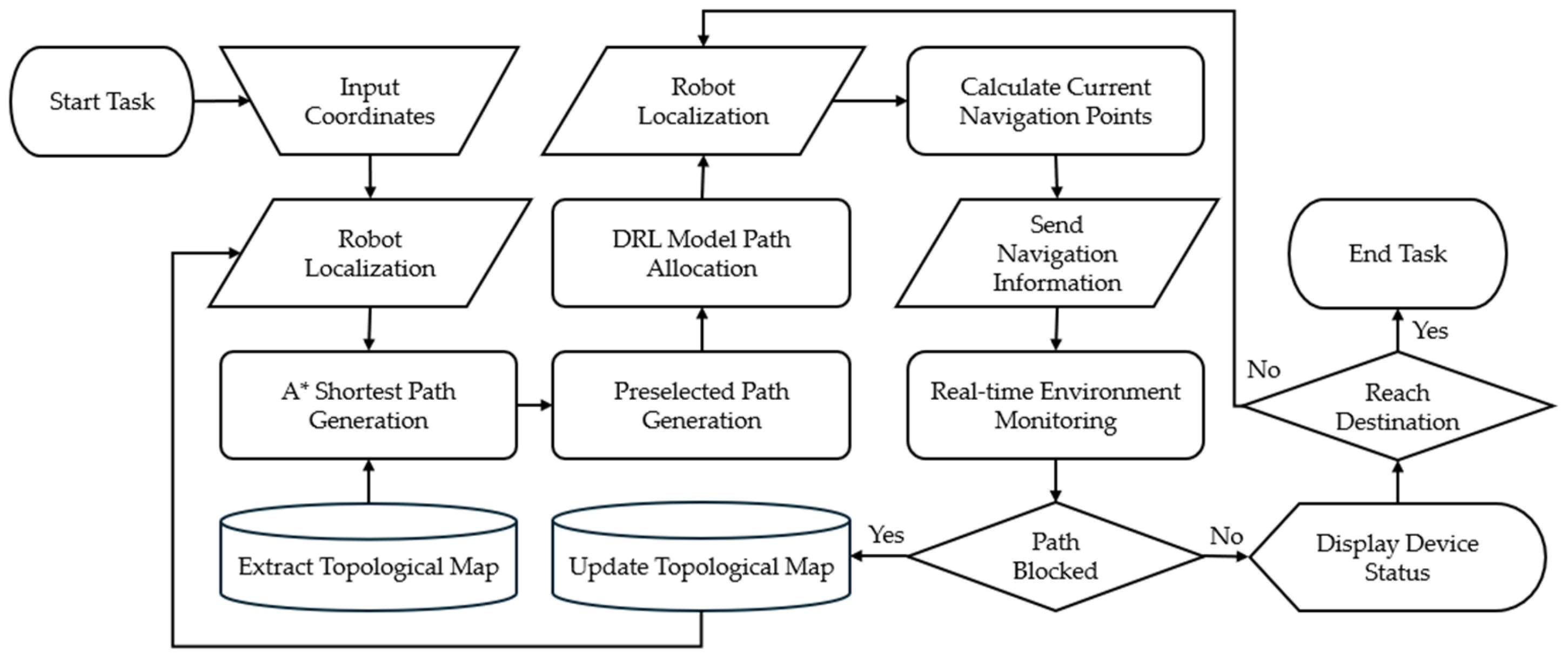
In the proposed multi-robot navigation system, there are four parts: (i) system architecture and process, (ii) environmental map representation, (iii) preselected path generation, and (iv) deep reinforcement learning model. They are described as follows.

3.1. System Architecture and Processes

In order to solve the path conflict problem and improve computing performance, the advantages of CBS and hierarchical architecture are combined. The architecture of the proposed multi-robot navigation system is shown in Figure 3. There are six main components: (i) localization unit, (ii) topological map, (iii) preselected path generation unit, (iv) deep reinforcement learning model, (v) path management unit, and (vi) environment monitoring unit. The localization unit is responsible for monitoring and managing the location of all robots and providing information about the coordinates of the robots in the preselected path generation unit and the path management unit. The topological map is responsible for recording and representing the current state of the environment. The preselected path generation unit is responsible for quickly planning several paths on the environment map and providing these preselected paths as follow-up options. The deep reinforcement learning model is responsible for selecting the optimal path for each robot, with the goal of finding a set of path combinations that minimize path conflicts. The path management unit is responsible for providing navigation information for each robot and guiding the robot through these arranged paths one by one. Finally, the environment monitoring unit is responsible for receiving the feedback data from the robots and updating the topological map with such data.

The system uses topological maps and A* algorithms to plan preselected paths, selects a path through a deep reinforcement learning model, and dynamically updates to ensure global optimization. This architecture is the application of a combination of methods. Although traditional CBS methods perform well in static environments, their computational complexity and scalability are limited when facing dynamic environments. Similarly, although distributed reinforcement learning methods have good adaptability in dynamic environments, they require a large amount of computing resources and training data. The proposed method combines the advantages of both methods and uses a deep reinforcement learning model to perform local path selection. This not only ensures the efficiency of path planning but also enhances the adaptability and robustness of the system in dynamic environments.

The system flow is shown in Figure 4. The start and end of the task represent the completion of the navigation task for all the robots. The start and end points of each robot are obtained by the user’s settings and the positioning system information, respectively. At the beginning of the planning process, the starting and ending points of all the robots are used to further plan three preselected paths for each robot using topological maps, A* algorithms, and other strategies. With the advantage of topological maps, the system can effectively reduce the computational cost and find the shortest path from the origin to the destination quickly through the A* algorithm. In this study, the three preselected paths are all equal in length. Then, the system selects the optimal path for each robot from the three preselected paths by means of a deep reinforcement learning model, which ensures that the combination of the selected paths achieves the approximate global optimal effect. Specifically, this ensures that each robot travels the shortest path from the origin to the destination, and the number of conflicting paths is close to the minimum. After obtaining the path of each robot, the system constantly knows the location of the robot through the positioning system and guides the robot. In addition, when the system carries out the navigation task, the robot will constantly report the current path status, and the system will update the topological map according to the situation and plan a new route for all the robots from scratch so that the system will achieve a better overall planning effect under the advantage of the whole situation.

3.2. Environmental Map Representation

In the environmental map representation, this study uses the topological map as the map representation method. The topological map represents the whole environment in a more advanced way and reduces the amount of computational data effectively. The complete topological map is obtained through the following three steps: (i) generating 2D occupancy maps, (ii) creating nodes, and (iii) creating edges and weights.

Firstly, this study uses NVIDIA Isaac Sim’s occupation map generator to generate a 2D occupancy map of the experimental environment. As shown in Figure 5a, the height range of the map is first specified by the generator. In this study, the origin, upper bound, lower bound, and cell size are set as shown in

Table 3. Occupancy map generator sampling range settings table.

Item	Start Point	Upper Bound	Lower Bound	Element Size
Value	(0.0, 0.0, 0.3)	(6.0, 2.0, 0.2)	(−42.0, −58.0, −0.2)	0.05

. As shown in Figure 5b, the occupancy situation within the specified boundaries will be generated, and this 2D occupancy map will completely and accurately display the objects in the environment with collisions enabled. Therefore, this step mainly focuses on obtaining the occupancy situation in the environment. And, in real-world scenarios, the 2D occupancy map can be obtained using engineering drawings or SLAM generation.

Secondly, after successfully obtaining the 2D occupancy map, the topological map can be constructed. In this study, the topological map is represented as an undirected graph $G$ and is expressed by

$$G=(V, E)$$

(1)

where $V$ is the set of nodes and $E$ is the set of edges. Each intersection is regarded as a node. When the node set $V$ contains 21 nodes, it can be expressed by

$$V=\{v_1, v_2, v_3, \dots , v_{21}\}$$

(2)

Finally, each node will be connected to the surrounding nodes, and the road between each intersection is regarded as an edge. In order to carry out further calculations later, this study assigns a specific weight on each edge as the cost of the length of each path. In this scene, the lengths of the vertical and horizontal axes of the iw.hub are about 6 units and 3 units, respectively. Therefore, the complete edge set $E$ is expressed by

$$E=E_{vertical}\cup E_{horizontal}$$

(3)

where $E_{vertical}$ and $E_{horizontal}$ are the vertical axis edge set and the horizontal axis edge set and are expressed by

$$E_{vertical}=\left\{\right\{\mathrm{1,2},6\},\{\mathrm{2,3},6\},\dots ,\{\mathrm{19,20,6}\},\{\mathrm{20,21,6}\left\}\right\}$$

(4)

and

$$E_{horizontal}=\left\{\right\{\mathrm{1,4},3\},\{\mathrm{4,7},3\}, \dots ,\{\mathrm{15,18,3}\},\{\mathrm{18,21,3}\left\}\right\}$$

(5)

As shown in Figure 6, a total of 21 nodes and 32 edges will be obtained, and each edge has its own weight.

Compared with the grid map, the topological map emphasizes the connection and relationship between locations rather than the precise physical distance or direction, which can greatly simplify the spatial representation and effectively reduce the spatial complexity and non-essential information. Meanwhile, the system in this study focuses on how to assign robots to move from one location to another; therefore, it only needs the reachability between these locations rather than the precise delineation of each location in the environment. Topological maps fully meet these conditions and achieve the complete representation of the system’s required mapping information in a much smaller amount of data.

3.3. Preselected Path Generation

In this study, the preselected path generation aims to plan three preference paths for each robot from the start point to the end point, one of which is generated by the A* algorithm, while the other two are simpler to use the preferred longitudinal path or preferred horizontal path, and this planning strategy is simple and effective to provide three flexible preference paths. The A* algorithm is a heuristic search algorithm, and the core of the algorithm is to find the minimum cost path by considering the known distance of the path and the estimated remaining distance at the same time during searching. The core of the algorithm is to find the minimum cost path by considering both the known distance and the estimated remaining distance of the path during the search process. Firstly, the start point $v_{start}$ and end point $v_{end}$ of the robot are defined and the start point $v_{start}$ is put into an open list $O$, which is used to store the nodes to be evaluated, as expressed by

$$O=\left(v_{start}\right)$$

(6)

and another closed list $C$ is used to store the evaluated nodes, as expressed by

$$C=\varnothing$$

(7)

In the search phase, new nodes around will be continuously added to the open list $O$, their total cost $f_{first}\left(n\right)$ will be calculated, and the node with the lowest cost will be further placed in the closed list $C$. The selection process is represented as

$$n=arg \underset{v\in O}{\mathit{min}}f\left(n\right)$$

(8)

In calculating the total cost $f_{first}\left(n\right)$, the first step is to determine whether the node is not included in the closed list $C$. If it is not included, then the calculation of the total cost f (n) is carried out, and the total cost consists of the actual cost from the starting point to the current node, which is expressed by

$$g\left(n\right)=g\left(m\right)+d_{Manhattan}(x_n, y_n, x_m, y_m)$$

(9)

and the estimated cost from the current node to the end point, which is expressed by

$$h\left(n\right)=d_{Manhattan}(x_n, y_n, x_{goal}, y_{goal})$$

(10)

In this study, we use Manhattan distance as the trigger function $d_{Manhattan}$, which is expressed by

$$d_{Manhattan}(x_1, y_1, x_2, y_2)=\left|x_1-x_2\right|+\left|y_1-y_2\right|$$

(11)

Therefore, in the actual cost $g\left(n\right)$, $g\left(m\right)$ represents the cumulative cost from the starting point to the current node, and the cost from the current node to the new node is calculated using the initiating function $d_{Manhattan}$. The estimated cost $h\left(n\right)$ is directly calculated from the current node to the end point using the heuristic function $d_{Manhattan}$. Finally, the actual cost and the estimated cost form the total cost $f_{first}\left(n\right)$, which is denoted as

$$f_{first}\left(n\right)=g\left(n\right)+h\left(n\right)$$

(12)

After calculating the total cost, the node with the lowest cost will be moved to the closed list $C$, and further checked whether it reaches the end point to determine whether to end the search or not, and if it does not reach the end point, then keep updating the open list and calculating the cost. Among them, this study does not use the weights mentioned in Section 3.1 in the path planning stage and treats the scattering of nodes in the map as uniform, so $d_{Manhattan}\left(x_n, y_n, x_m, y_m\right)$ can be directly regarded as one.

For the other two preselected paths, this study uses a simpler way to plan the paths, and each of them follows the priority of traveling in the vertical or horizontal direction, and the actual cost of $g_{vertical}$ when traveling in the vertical axis only takes the moving distance in the y-axis direction into account, which is expressed by

$$g_{vertical}\left(n\right)=\left|y_n-y_{goal}\right|$$

(13)

The actual cost $g_{horizontal}$ when traveling in the horizontal direction only considers the moving distance in the x-axis direction, which is expressed by

$$g_{horizontal}\left(n\right)=\left|x_n-x_{goal}\right|$$

(14)

The sum of the two is the total cost $f_{others}\left(n\right)$, denoted as

$$f_{other}\left(n\right)=g_{vertical}+g_{horizontal}$$

(15)

Therefore, the length of the paths planned by the A* algorithm and the preferred walking strategies on the vertical and horizontal axes are the same, and because of this, the length of the paths is the same for all cases when the deep reinforcement learning model is allowed to choose the paths in Section 3.4. One example of three preselected paths is shown in Figure 7. The paths selected by the A* algorithm, the vertical axis priority strategy, and the horizontal axis priority strategy are shown in Figure 7a–c, respectively.

3.4. Deep Reinforcement Learning Model

In this study, the deep reinforcement learning model is the key component for selecting one path for each robot from each of the three preselected paths planned for each robot in Section 3.3. There are two parts: (i) environment modeling and (ii) algorithm and model architecture. They are described as follows.

In environment modeling, this study introduces how to model the path selection problem, including the inputs, outputs, and learning objectives of the deep reinforcement learning model; in other words, this subsection introduces the observation space, action, and reward of deep reinforcement l1earning.

First, the environment will continue the topological map content in Section 2.2, set as shown in

Table 4. Parameter settings for deep reinforcement learning.

Item	Value
Environment Size	7 × 3
Number of Robots	10
Number of Candidate Paths	3
Length of Candidate Paths	12

, a 7 × 3 size node map with 10 robots. In this environment, the state S consists of the state $S_i$ of each robot, denoted as

$$S=\{S_1, S_2, S_3, \dots , S_{10}\}$$

(16)

and the state $S_i$ of each robot contains three preselected paths $P_{i1}$ to $P_{i3}$ of each robot, denoted as

$$S_i=\{P_{i1}, P_{i2}, P_{i3}\}$$

(17)

To ensure a consistent state size, each path is standardized to contain 12 nodes. In the case that the number of nodes is insufficient, it will be filled to a fixed length of 12 by zero padding; thus, it is expressed by

$$P_{ij}=\{p_{ij}^1, p_{ij}^2,p_{ij}^3, \dots , p_{ij}^{12}\}$$

(18)

where

$$p_{ij}^k=\left\{\begin{array}{c} n, \mathrm{if} k\le l_{ij} \\ 0, \mathrm{if} l_{ij}<k \le 12\end{array},n\in \mathbb{N}\right.$$

(19)

and $l_{ij}$ denotes the actual number of nodes in the $j$th preselected path of the i-th robot. Thus, the actual state dimensions will be ten robots and three preselected paths, and the length of the preselected paths is twelve, which describe the location of each robot and its preselected paths and provide the model with the complete information needed for decision making.

In this setting, action A describes the model as the path chosen by each robot; specifically, the dimension of action A is fixed to ten (the number of robots), which selects a path for each robot from the three preselected paths that is the best path for the whole, denoted as

$$A=\{a_1, a_2, a_3, \dots , a_{10}\}$$

(20)

where

$$a_i\in \{0, 1, 2\}, i=1,2,\dots ,10$$

(21)

The integer values 0, 1, and 2 are used to represent the first, second, and third preselected path, respectively. Thus, the action $a_i$ describes the path selection of the i-th robot.

The purpose of the reward $R$ design is to guide the model to select the optimal path combinations to minimize the number of intersection conflicts between robots. Specifically, in this study, the design of the reward function in the deep reinforcement learning model is very simple, and the reward R is expressed as

$$R=c_{standard}-c_{present}$$

(22)

It only takes into account the difference between the total number of standard actions of all the robots, $c_{standard}$, and the total number of current actions, $c_{present}$, which is a more direct response to the advantages and disadvantages of the current path combinations. In the calculation of the total number of conflicts, this study considers the current position of the robot at each time point, such as at the same time point at the same node where there are n sets of robots located in the same node, and the number is greater than 1; then, it is regarded as n times of conflict. First, each path needs to be developed to obtain the time point when the robot passes through each node, where the weight set by the topology is considered, which is used as the basis for calculating the node and time pair $T_i$ that will be obtained, including the position information and time information, expressed as

$$T_i=\left\{\left(p_{ij}, t_{ij}\right) \right| t_{ij}=t_{i(j-1)}+distance(p_{i(j-1)}, p_j)\}$$

(23)

Furthermore, the set of all robots $T_{p,t}$ located at node $p$ at each time point $t$ is counted and is denoted as

$$T_{p,t}=\left\{i | (p_{ij}, t_{ij}) \in T_i ,p_{ij}=p, t_{ij}=t \right\}$$

(24)

and, finally, obtains the total number of collisions $c$ in

$$c={\sum }_t{\sum }_p\left(\right|P_t\left(p\right)|·1(\left|P_t\right(p\left)\right|>1\left)\right)$$

(25)

In this study, we use proximal policy optimization (PPO) [30] as the algorithm for deep reinforcement learning. It is based on the actor-critic architecture, which consists of two main components: the actor and the critic. The actor is responsible for determining the actions to be taken in each state by learning a policy function. The critic is responsible for evaluating the quality of these actions by learning a value function that estimates the expected returns following the current policy in the given state. PPO replaces the traditional policy gradient objective with a clipped surrogate objective function. This objective function considers the ratio between the current policy gradient and the old policy gradient and clips the ratio when it exceeds a certain range. This approach limits the magnitude of policy updates, avoiding instability caused by excessive policy changes and thereby improving training stability and effectiveness. Concurrently, the actor updates the policy by maximizing the clipped objective function, while the critic updates the value function by minimizing the mean squared error between predicted and actual returns. This process helps evaluate the performance of the current policy and provides the actor with the basis for policy updates, which is expressed by

$$L^{CLIP}\left(\theta \right)=E[min (r_t\left(\theta \right){\hat{A}}_t, clip(r_t\left(\theta \right), 1-\epsilon , 1+\epsilon ){\hat{A}}_t\left)\right]$$

(26)

where $r_t\left(\theta \right)$ is the ratio between the probability of the old and new strategies, ${\widehat{A}}_t$ is the advantage function, and ε is the hyperparameter that controls the cropping range. By limiting the magnitude of strategy updating, this approach avoids the instability that may be caused by too large a strategy change, thus improving the stability and effectiveness of training. Meanwhile, PPO is designed based on the actor-critic architecture, where the actor is responsible for inputting the action strategy and updating the target function by maximizing the pruned strategy target function, while the critic is based on the state-value function and updating it by minimizing the mean squared error, which is useful for evaluating the performance of the current strategy. The main purpose is to help evaluate the performance of the current strategy and to provide an updated strategy for the actors.

In the model architecture, this study adopts the Multi-Layer Perceptron (MLP) architecture, in which the neurons in each layer are fully connected with all the neurons in the previous layer so that the MLP can efficiently simulate high-dimensional and non-linear function relationships. In the experiments, the number of neurons in the input layer is 360, with a total of 21 nodes, 10 robots, and a default maximum path of 12. In this case, we simply design two hidden layers with sixty-four neurons each and use the Rectified Linear Unit (ReLU) as the activation function of the neurons. Finally, the model has a total of 10 outputs to select paths for 10 robots.

4. Simulation Results and Discussion

This study designed some experiments to evaluate the performance of the proposed system. In addition, experiments are performed in NVIDIA Isaac Sim to obtain experimental results that closely resemble real-world scenarios. In the system evaluation experiment, the system’s ability to reduce path conflicts and its operating efficiency under different map sizes and the number of robots are mainly evaluated. This experiment demonstrates the significant impact of the concept of reducing path conflicts, while in feasibility evaluation experiments, the main goal is to verify the practical feasibility of the proposed system.

4.1. System Evaluation Experiment

This study designed nine simulation conditions, as shown in

Table 5. Nine simulation conditions.

ID	Map Size	Number of Nodes	Robot Ratio	Number of Robots
E1(13)	5 × 5	25	50%	13
E1(25)	5 × 5	25	100%	25
E1(38)	5 × 5	25	150%	38
E2(50)	10 × 10	100	50%	50
E2(100)	10 × 10	100	100%	100
E2(150)	10 × 10	100	150%	150
E3(113)	15 × 15	125	50%	113
E3(225)	15 × 15	125	100%	225
E3(338)	15 × 15	125	150%	338

. Each condition differed in map size and number of robots, labeled E1(23) to E3(338). The map size is divided into three scenarios: small, medium and large, corresponding to node arrangements of 5 × 5, 10 × 10, and 15 × 15. The map node diagram is shown in Figure 8. The horizontal and vertical axes distances between each node in the map are set to three and six time steps, respectively. The main consideration is the realistic map size and the number of robots. Usually, this number of robots can operate better and will not be too crowded or insufficient to cope with transportation needs. Therefore, the number of robots is set in corresponding proportions based on these scenarios, including 50%, 100%, and 150% of the corresponding number of nodes. These settings help simulate the dynamic characteristics of the real environment.

In the simulation results of 1000 times, the numbers of path conflicts in nine simulation conditions are shown in Figure 9. For the part of the number of conflict improvement, E1(13) to E3(338) have about 15,451 and 2,139,331 collisions, respectively, in 1000 plannings. We can see that when the complexity of the environment and the number of robots increases, the number of path conflicts increases significantly. This highlights the important concept proposed in this study to reduce the number of path conflicts.

As shown in Figure 10 and

Table 6. Statistics table on the number of path conflicts and improvement effects in nine experimental conditions.

ID	Number of Path Conflicts Using A* Method	Reduced Number of Path Conflicts	Collision Reduction Ratio	Total Navigation Time Saved by the Proposed Method (h)
E1(13)	15,451	1520	9.84%	1.27
E1(25)	49,691	2483	5.0%	2.07
E1(38)	96,064	2671	2.78%	2.23
E2(50)	103,857	6786	6.53%	5.66
E2(100)	347,384	13,073	3.76%	10.89
E2(150)	660,615	18,048	2.73%	15.04
E3(113)	339,946	17,859	5.25%	14.88
E3(225)	1,116,827	42,918	3.84%	35.77
E3(338)	2,139,331	60,375	2.82%	50.31

, the number of path conflicts and improvement effects in nine experimental conditions are described. We can see that the deep reinforcement learning model reduces the ratio of reduced path conflicts for E1(13) and E3(338) by about 9.84% and 2.82%, respectively. If it takes about 3 s for a robot control system to resolve the path conflict once, the navigation time for E1(13) and E3(338) can save 1.27 h and 50.31 h, respectively. The main reason for this is that the increase in robot density makes it difficult for the model to select a better combination of paths; the preselected paths used in this study are relatively one-dimensional, and more complete preselected paths may further improve the model’s capability.

In the part of resource utilization, as shown in Figure 11, the graph’s vertical axis represents the time in milliseconds. As the map size and the number of robots increase, the system response time also increases proportionally. However, it can be observed that the inference time of this system model is very short compared to the inference time of the overall system. It can be observed that the model inference time for E3(338) takes only 0.19 ms, but the inference time of the whole system takes 38.50 ms. Therefore, most of the system time is spent on other functions, such as preselected path generation and path management. It can be observed more clearly in Figure 12 that with the rise of the complexity of the environment and the number of robots, the inference time of the system is much higher than that of the model. Figure 12 shows that the inference time of the system is much higher than that of the model when the complexity of the environment and the number of robots is increased. If further optimization of performance is needed in the future, other functions can be improved first. On the other hand, under the two simulation conditions of E1(13) and E3(338), according to the conversion of the model and system inference time, we can obtain an operation efficiency of about 1538.46 FPS and 20.58 FPS, respectively. Therefore, if we need to change the path immediately or even carry out the planning in a dynamic way, the current efficiency of the system can be fully capable of handling it, which confirms the feasibility of the system proposed in this study.

In the model training part, as shown in Figure 13, the horizontal axis in the figure represents the experimental conditions, and the horizontal axes represent training time and FPS, respectively. Under the conditions of a small environment, a stable model can be obtained in about 0.48 h. This training process is trained at a speed of about 1020 FPS, while under the conditions of a large environment E3(338) with 225 nodes and 338 robots, it takes about 28.58 h of training to obtain a stable speed model, and this process takes about 101 FPS.

Summarizing the above, the system proposed in this study has a good performance in reducing the number of path conflicts and efficiency; especially, regarding efficiency, it can re-plan all the robots’ paths in a very short time, and the planned paths are close to the best results in the whole domain. Most importantly, the system does find a new way to solve the path conflicts by reducing the number of path conflicts instead of simply solving the path conflicts through obstacle avoidance.

4.2. Feasibility Assessment Experiment

As shown in Figure 14, a simulation scenario with 24 neatly arranged shelves and 10 Idealworks iw.hubs is designed to simulate the movement of 10 robots in a warehouse to verify whether the system proposed in this study can smoothly guide 10 robots at the same time, and the local path algorithm named reciprocal velocity obstacles (RVOs) [31] is combined to avoid each other at the path conflict points. The state definition for the system evaluation is shown in

Table 7. State definition for the system evaluation and evaluation of the simulation results of 10 robots in an environment with 24 shelves.

State	Definition	Value
Success	No collisions occurred	49
Stopped	No collisions occurred but the task was not completed	1
Danger	Collisions occurred but the task was completed	0
Failure	Collisions occurred and the task was not completed	0

. A complete navigation without any collision will be considered a success, a collision but still completing the mission will be considered a danger, and a collision and not completing the mission for that navigation will be considered a failure, and the number of collisions will continue to accumulate for each collision. The evaluation of this simulation of 10 robots in an environment with 24 shelves is shown in Table 7. In a total of fifty experiments, forty-nine were successful and one was stopped, achieving a success rate of 98%. The only major reason for failure was the possible collision of multiple robots with the field equipment during path congestion, resulting in the stoppage of the robots. One of the simulation videos can be viewed on this website: https://youtu.be/oPmJAwGHg70, accessed on 21 August 2024. In this simulation scenario, the start point and the end point of each robot are randomly generated, and the start point state is shown in Figure 14a, while the end point state is shown in Figure 14b, and the experiment is carried out for a total of 50 times. We can see that all robots effectively move from the start points to the end points.

5. Conclusions

This study designs a multi-robot navigation system. A path planning and selection method based on deep reinforcement learning is proposed to plan paths with fewer path conflicts for all robots. This study has two advantages. First, this study uses topological maps to simplify the map representation for multi-robot path planning. Since the number of nodes used in the topological map is small, the implemented system does not occupy too many computing resources. This enables the proposed method to perform path planning for more robots in more complex environments. Second, this study employs the A* algorithm and combines other policies for path generation. The PPO algorithm is used for path selection, which can effectively reduce path conflicts in multi-robot navigation. Experiments using three different map sizes and different numbers of robots show that the proposed method has good real-time performance and good computational efficiency. The experimental results show that its performance ranges from a minimum of 20.58 FPS to a peak of approximately 1538.46 FPS. In addition, it also significantly reduced the number of path conflicts. The experimental results show that the maximum number of path conflicts that can be reduced is 60,375. In 1000 multi-robot navigation tasks, it can reduce the number of path conflicts by 9.84%. The fewer path conflicts between multiple robots, the less navigation time it takes for the robots to complete all tasks. For busy warehouses, a method that can save a lot of overall navigation time is very important. From the perspective of multi-robot global path planning, the proposed method is already a phased contribution. For local path planning on the robot, the existing RVO algorithm is used to prove the effectiveness of the proposed method in global path planning. In future work, we will also try to use DRL methods to design a more effective local path planning method so that the robots can more effectively avoid each other at the path conflict points and avoid obstacles dynamically on the planned path.