Design, Building and Deployment of Smart Applications for Anomaly Detection and Failure Prediction in Industrial Use Cases

Abstract

This paper presents a comparative analysis of deep learning techniques for anomaly detection and failure prediction. We explore various deep learning architectures on an IoT dataset, including recurrent neural networks (RNNs, LSTMs and GRUs), convolutional neural networks (CNNs) and transformers, to assess their effectiveness in anomaly detection and failure prediction. It was found that the hybrid transformer-GRU configuration delivers the highest accuracy, albeit at the cost of requiring the longest computational time for training. Furthermore, we employ explainability techniques to elucidate the decision-making processes of these black box models and evaluate their behaviour. By analysing the inner workings of the models, we aim at providing insights into the factors influencing failure predictions. Through comprehensive experimentation and analysis on sensor data collected from a water pump, this study contributes to the understanding of deep learning methodologies for anomaly detection and failure prediction and underscores the importance of model interpretability in critical applications such as prognostics and health management. Additionally, we specify the architecture for deploying these models in a real environment using the RAI4.0 metamodel, meant for designing, configuring and automatically deploying distributed stream-based industrial applications. Our findings will offer valuable guidance for practitioners seeking to deploy deep learning techniques effectively in predictive maintenance systems, facilitating informed decision-making and enhancing reliability and efficiency in industrial operations.

1. Introduction

Over the past five years, the integration of artificial intelligence (AI) into predictive maintenance has profoundly transformed the industrial sector. The synergy between advanced technologies, such as real-time data analytics and low-cost sensors, combined with machine learning models, has enabled the unprecedented precision in anticipating failures in complex systems. This approach not only optimises maintenance intervals but also enhances reliability and reduces operational costs [1]. Even more, developments in sophisticated algorithms, alongside human expertise, have enabled the creation of models that not only predict failures but also suggest specific corrective actions, thereby minimising downtime and repair costs [2].

There are many different strategies to build predictors but the ones that are currently producing the best results are those supported by deep learning techniques [3]. Therefore, we will focus on the analysis and comparison of different algorithms applied to a case study of anomaly detection and failure prediction. In addition, we will work with explainability techniques, known by the acronym XAI (explainable AI), [4] to determine the factors or variables that most influence the prediction of failure. These AI models work well because the volume of data available is huge and computation power is high thanks to the lower cost of hiring cloud nodes.

However, it should not be forgotten that not only is it necessary to build the model, but also to deploy and monitor it in order to detect when the model becomes less accurate and needs to be updated. This is absolutely essential when working with continuous data streams that may be affected by concept drift [5]. This term means that the statistical relationships between input variables and model output variables change over time, which can deteriorate model performance if not properly detected and managed. This leads us to think not only about the model but also about the technological platform needed to ensure that the model’s life cycle is fully automated [6].

In this regard, having tools that facilitate the design and deployment of the predictive system as well as its monitoring to update the model when it is underperforming is very practical and essential for companies. In this sense, we describe our use case using the RAI4.0 metamodel [7] which allows us to specify the different elements that make up the digital platform that will host the prediction service along with their deployment parameters. Working with models (model-based engineering) provides considerable advantages, not only in terms of reasoning on and documenting our digital platform, as well as in terms of time saved when deploying and re-deploying with different configurations. Likewise, the time required for the integration of new applications or services is reduced since parts of the model can be reused.

In short, this paper has two main objectives. Firstly, it conducts a comparative study of deep learning techniques for constructing failure predictors in sensorised devices and uses explainable AI (XAI) algorithms to better understand their behaviour. Secondly, it seeks to present an automated strategy for the deployment and performance monitoring of these predictors, utilising a MLOps architecture framework [6].

The outline of the paper is as follows: Section 2 provides an overview of the predictive maintenance arena, including its aim, problem types and techniques to address them, making a special focus on anomaly detection and failure prediction. Section 3 presents our case study, detailing the data description, the preprocessed tasks performed and the setting of different deep learning algorithms to build an anomaly predictor service discussing its performance. Next, Section 4 explains the most effective XAI techniques that are applied for different purposes, such as understanding false positives or identifying components causing the failures. Section 5 discusses the findings of this study regarding deep learning and XAI. Section 6 describes the platform deployed to support the predictive maintenance service and its monitoring. Finally, Section 7 draws the conclusions of the paper and the next steps in our research.

2. Data-Driven Predictive Maintenance

According to the European standard EN 13306:2010, maintenance is defined as “the combination of all technical, administrative and managerial actions during the life cycle of an item intended to retain it in or restore it to a state, in which it can perform the required function” [8]). Further, maintenance can be divided into three main categories: corrective, preventive and predictive maintenance.

Predictive maintenance (PdM) is an evolution of the previous two maintenance protocols. Unlike simpler forms of maintenance such as corrective maintenance, which performs no tasks until a failure occurs, or preventive maintenance, which relies on mean time between failures to establish a maintenance schedule, predictive maintenance utilises monitoring data to infer the actual condition of a system. This last approach allows for the detection or prediction of failures, enabling more effective scheduling of maintenance tasks. Consequently, it reduces downtimes, improves the health status management of industrial equipment and maximizes their useful life [1,9].

The term “data-driven” enhances PdM by incorporating historical data to build models that guide decision-making. In essence, it involves identifying patterns, correlations, and anomalies to provide insights into equipment health and performance. This approach requires, on the one hand, datasets that include representative and effective observations of degradation, failures, and even complete failure performance data, which can be challenging to achieve [3]; and on the other hand, advanced computational techniques, such as those from deep learning arenas, to build these models, which require qualified professionals [10].

Before briefly describing these techniques, we mention the usual maintenance strategies under which data driven predictive maintenance problems are classified [11]: (1) anomaly detection, (2) failure diagnosis, (3) remaining useful life prediction (RUL) and (4) mitigation. The first one involves detecting potential failures that have just occurred or are about to take place. Failure diagnosis aims to identify the true cause of a problem and is usually addressed by applying root cause analysis (RCA) techniques. Next, the estimation of the remaining time or, in other words, cycles until a failure occurs should be carried out. Finally, all this information would be communicated to industrial engineers in order to implement a mitigation plan.

We can find many applications and use cases representative of each stage in the literature. For instance, ref. [12] introduces an innovative framework that harnesses a hybrid approach, uniting convolutional neural networks (CNN) and long short-term memory networks (LSTM), referred to as CNN-LSTM, to predict component failures in air production units (APUs) installed in metro vehicles. Lei et al. [13] present a novel fault diagnosis framework for wind turbines using an end-to-end long short-term memory (LSTM) model. Its results demonstrate that this method effectively classifies faults from raw time-series signals collected by single or multiple sensors, outperforming state-of-the-art approaches. Li et al. [14] focus on the importance of accurately predicting the remaining useful life (RUL) of lithium-ion batteries using machine learning (ML) algorithms, discussing the general process of RUL prediction and comparing the top ten algorithms based on accuracy and characteristics. Taşcı et al. [15] proposed a hybrid model for predicting the remaining useful lifetime before production lines stop. They used real-world high-dimensional data from IoT sensors and among all the proposed methods, RF (random forests), an ensemble bagging method, turned out to perform best. They did not use deep learning algorithms. On the other hand, autoencoder-based methods have been also tested successfully for novelty detection, another major challenge in industrial plants, where both operational conditions change over time and a large number of unknown modes occur [16]. The number of works is very extensive—the interested reader can find more case studies in current surveys written by different authors [1,2,17,18,19].

Another recent and interesting paper that guides scientists to select a suitable deep learning architecture is [3]. This classifies techniques according to four dimensions: (1) target of the task, such as degradation assessment, RUL prediction, health estimation and damage identification; (2) the features that may need to be extracted, including time dependency features, complex representations, discriminatory features and hierarchical representations; (3) the input data, including coupled or disordered levels, data types, and relationships between neighbouring variables; and (4) special demands on analysis capability, including the capabilities to deal with temporal information, complex environments, and complex imagery scenes. Following its roadmap, we included RNN, LSTM and CNN in our benchmark.

Recently, researchers from Milano University [20] investigated the failure prediction task in industrial datasets considering the impact of both the reading window length and the prediction window length. For this purpose, they compared different machine learning and deep learning algorithms and concluded that deep learning outperforms machine learning when the complexity of the dataset increases as measured by the average spectral entropy.

Next, we overview deep learning techniques used for anomaly detection and failure prediction.

Anomaly Detection and Failure Prediction

This section focuses on the study of anomaly detection using deep learning techniques, specially recurrent neural networks and convolutional neural networks. According to [11] the most employed and better performing models in PdM tasks are:

• Recurrent neural networks (RNNs) [21], a type of artificial neural network designed to recognise patterns in sequences of data. Unlike traditional neural networks, RNNs have loops that allow information to persist, making them well-suited for sequential data processing.
  RNNs have a unique architecture where connections between nodes form a directed cycle. This allows the network to maintain a ’memory’ of previous inputs. The simplest form of RNN can struggle with long-term dependencies due to issues like the vanishing gradient problem, therefore architectures such as long short-term memory (LSTM) and gated recurrent unit (GRU) were created with gate mechanisms to regulate the flow of information and to capture long-term dependencies efficiently. These are used for time-series forecasting, natural language processing (NLP) or recommender systems. Figure 1 shows the structures of the different RNN cells. The simpler RNN cell receives the current time-step and the output from the previous time-step as input, so several time-steps are taken into account for each model prediction. However, these simpler cells face two main problems that affect their ability to capture long-term relationships in the data: vanishing gradient and exploding gradient. The former is caused by gradients rapidly approximating to zero and thus stopping the training process. Whereas the latter is the opposite, gradients grow towards infinity making the training process highly unstable and provoking the appearance of NaN values. To solve these problems, LSTM cells introduce cell states to mitigate the vanishing gradient problem and a three gate system to manage the state. The input gate determines how much of the new information is incorporated into the cell state, the forget gate determines which information is discarded from the cell state and, finally, the output gate determines what information is forwarded. Moreover, GRU cells follow the same principle as LSTM, keeping an internal state or memory, but they are designed using only two gates to improve efficiency. The update gate controls how much from the previous state should be kept and how much of the new information should be included and the reset gate determines how much of the hidden state has to be forgotten.

Figure 1. RNN, LSTM and GRU cells architecture [22].

Figure 1. RNN, LSTM and GRU cells architecture [22].

• Convolutional neural networks [19], a class of deep learning models particularly well-suited for computer vision and natural language processing. They are fully connected feedforward neural networks with convolutional and pooling layers. The former applies a set of filters (or kernels) to the input image, generating feature maps that highlight various characteristics such as edges, textures, and patterns, and the latter reduce the spatial dimensions of the feature maps, typically using operations like max pooling or average pooling, which helps to reduce computational load and to achieve spatial invariance. For time series forecasting and classification, a special type of CNN called a one-dimensional convolutional neural network (1D CNN) is usually employed. This kind of CNN uses one-dimensional filters that convolute only over the time axis (as shown in Figure 2), allowing the identification of temporal patterns in the data.

Figure 2. Simple 1D convolutional neural network (CNN) architecture with two convolutional layers [23].

Figure 2. Simple 1D convolutional neural network (CNN) architecture with two convolutional layers [23].

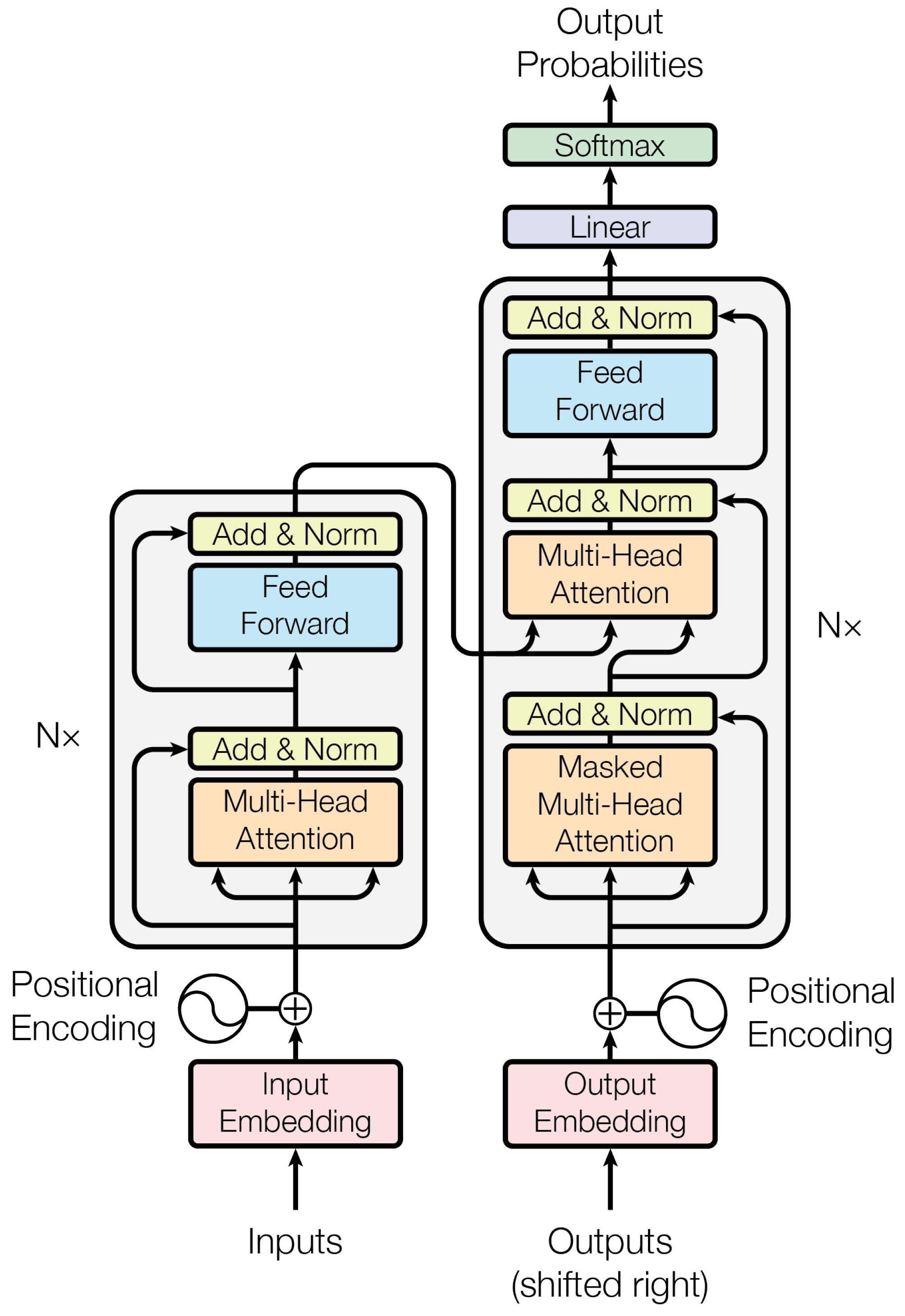
• Generative models, a class of machine learning models that learn to generate new data samples that resemble a given dataset. Unlike discriminative models, which learn the boundary between classes, generative models learn the underlying distribution of the data. There are different types, some of the most relevant are the following: (1) Deep belief networks (DBN) which are hierarchical generative models composed of multiple layers of RBMs (restricted Boltzmann machines) and generally used for unsupervised learning tasks and as feature extractors. (2) Generative adversarial networks (GANs) that consist of two neural networks, the generator and the discriminator, which are trained simultaneously in such way that the generator tries to fool the discriminator, while the discriminator aims to correctly identify the real and generated data. The objective of the generator is to maximise the discriminator’s error rate. (3) Variational autoencoders (VAEs) encode data into a latent space and then decode it back to reconstruct the data. VAEs are particularly popular for tasks like image generation, data representation, and generating new samples that resemble the training data. Finally, (4) transformers, presented in [24], are composed of an encoder and a decoder, each of which is made up of several multi-head self-attention layers and feedforward layers (see Figure 3). These have recently become extremely popular for its use in machine translation and for being the base of well-known large language models (LLMs) such as GPT. However, with some adjustments they can also be applied to temporal and spatial data.

Figure 3. Transformer architecture [24].

Figure 3. Transformer architecture [24].

Additionally, it is remarkable to point out that anomaly detection techniques also have the potential to improve prognostics models in two ways: by removing noisy or erroneous data; and by detecting relevant events that can be used as new input features for the prognostics models, making it possible to have more generalised models [25].

3. Deep Learning Algorithm Comparison: Case Study

The purpose of this section is to apply different deep learning algorithms on a free available time series dataset from the Kaggle repository (https://www.kaggle.com/datasets/nphantawee/pump-sensor-data (accessed on 2 September 2024)) in order to compare their performance and suitability for anomaly detection.

This dataset is comprised of a set of measurements taken by the 52 sensors installed in a water pump responsible for supplying water to a small village. The owner of the system published the data with the purpose of being able to understand or detect failures as quickly and as accurately as possible in order to improve the service given to the village population. In the previous year, there were seven system failures that caused severe problems to the families living there. We did not have access to the real machine, so we simulated the behaviour of the system streaming a sample of the dataset at a constant rate.

Firstly, we set our goal to know when the water pump can fail with the aim of avoiding serious living problems that water outages involve. Briefly, to develop a predictive model capable of processing data in real time and determine if the water pump is operating normally or if, on the contrary, it has a malfunction that could lead to a pump failure.

3.1. Feature Selection

The dataset contains 220,320 records, made up of 52 numeric variables corresponding to different sensors collected every minute and the target variable which gathers the machine status. These are enumerated in Appendix A. The latter is a categorical variable which takes three possible values: NORMAL, BROKEN and RECOVERING. As a consequence of the low number of failures—only seven instances reported in the whole dataset—where a failure begins with a BROKEN status and is followed by a RECOVERY status before returning to NORMAL, instances with either BROKEN or RECOVERING statuses were both categorised as MALFUNCTION. Therefore, we approached the problem as a binary classification so the predictor could generalise better and become more useful. The remaining values received from sensors are supposed to be in a fixed range which should be stable and does not vary over the time. Thus, we consider that the dataset is not affected by concept drift (i.e., the value changes over time in unforeseen ways).

Next, for the feature selection step we took a simple approach, splitting the training data into run-to-failure experiments and eliminating the features that remained constant during the observation and showed no degradation trends overtime. We also removed the faulty sensor (sensor_15) that only reported null values. After that, we worked with 27 variables which were scaled using the MixMaxScaler algorithm offered by the scikit-learn library so all the variables fell within the same range. Then, as the percentage of data rows containing null values was only a 0.06% of the total, the replacement of missing values was addressed using a forward fill approach, i.e., applying the last observed value. Finally, as the algorithms to be employed require sequences as input, the data were rearranged using a sliding window approach with a window size equal to 60 time-steps and a step equal to 1 (each temporal instant).

3.2. Modelling

Next, five deep learning models capable of detecting water pump failures were built. We used the following algorithms: RNN, LSTM, GRU, 1-D CNN and a hybrid model based on a transformer encoder and a GRU (see Section 2). This last model uses the encoder part of a transformer architecture followed by a GRU neural network. This approach is proposed because it leverages the feature extraction and generation capabilities of the multi-head attention layers in the transformer’s encoder, while also harnessing the strength of recurrent neural networks in capturing temporal dependencies within the data. The sklearn 1.5.0 and Keras 3.5.0 software libraries were used for this purpose (Resources can be found in https://scikit-learn.org (accessed on 2 September 2024), https://keras.io (accessed on 2 September 2024) and https://www.tensorflow.org (accessed on 2 September 2024), respectively).

The parameter initialisation was performed by means of a grid search method, which consists of defining a matrix containing a list of possible options for each parameter and training the model with each different combination to find the best one.

The evaluation of the models was carried out using a 70/30 train/test split and applying k-fold cross-validation on the training set. This technique outperforms others such as leave-one-out or hold-out when the dataset has a number limited of instances (malfunction state in this case study) as empirically demonstrated by [26]. K-folds works as follows: the training set is split in k equal-sized subsets, then the model is trained using one of them as validation set and the rest as training set, repeating this k times until each subset has been used as a validation set.

The preprocessing pipelines and the models were built following traditional offline techniques, i.e., by means of a data sampling and training model from an historical dataset.

Table 1. Model configurations and training parameters obtained through grid search optimisation.

	RNN	LSTM	GRU	CNN	Transformer
Input size	(27, 60)
Output size	(2)
No of RNN layers	2	2	2	-	1
No of RNN cells	20/20	20/12	16/16	-	10
AF of RNN cells	tanh	tanh	tanh	-	tanh
No of CNN layers	-	-	-	1	-
AF of CNN layers	None	None	None	-	None
No of Filters	-	-	-	16	-
No of MHA layers	-	-	-	-	1
AF of MHA layers	None	None	None	-	None
No of Heads	-	-	-	-	5
No of FC layers	1	1	1	1	2
AF of FC layers	Softmax	Softmax	Softmax	Softmax	RELU/Softmax
No of Cells	2	2	2	2	10/2
Dropout rate	0.2
Batch size	32
Epochs	1000
Optimiser	Adam
Learning rate	0.001
Loss metrics	Binary Crossentropy

shows the configuration and training parameters chosen after performing the grid search. The network configuration parameters include: the size of the input and output data, the number of layers and cells of each type, the activation function (AF) (also known as transfer function) and the dropout rate (rate of ignored links between cells of different layers) used in the intermediate dropout layers to reduce over-fitting. The training parameters include the following: the number of data instances used in each training iteration known as batch size, the number of times that the training dataset is shown to the model or epochs, the model optimisation algorithm, the learning rate that controls how much the weights of the model are updated after processing each batch of data and the loss metric that the optimiser tries to minimise.

3.3. Evaluation Metrics

As a consequence of the imbalanced nature of machine failure data, we cannot rely on the accuracy of model as a quality measurement of the prediction. Thus, we used F1-score (see Equation (2)) which is computed based on recall and precision (see Equation (1)). These are computed using true positives (TP), i.e., positive cases correctly identified by the model; false positives (FP), i.e., negative cases mistakenly predicted as positives; and false negatives, i.e., positive cases mistakenly predicted as negatives. This takes into account the ratio of positive to negative test cases, making it a more suitable option for imbalanced datasets. In addition, we have included the training and inference time for each of the models built which can be determinant in soft real-time scenarios like this where we are trying to identify the failures as soon as possible.

$$Precision={\displaystyle \frac{TP}{TP+FP}}Recall={\displaystyle \frac{TP}{TP+FN}}$$

(1)

$$F1=2\ast {\displaystyle \frac{Precision\ast Recall}{Precision+Recall}}$$

(2)

3.4. Results

Table 2. Performance metrics.

Model	F1-Score	Training Time (s)	Inference Time (s)
RNN	0.566	191.5	0.036195
LSTM	0.947	439.7	0.036543
GRU	0.829	294.5	0.037423
CNN	0.915	79.87	0.035027
Transformer	0.964	602.6	0.037204

contains the F1-score achieved by each model after performing a three-fold stratified cross-validation as well as the training and inference times. We chose three-fold cross-validations due to the fact that the dataset contains highly imbalance data and this ensures that the proportion of normal and broken values is preserved while keeping enough broken cases in each subset.

The results confirm that LSTM is the most accurate recurrent architecture, as stated in [3], and that GRU is the most time-efficient, as explained in Section 2. However, our hybrid transformer-GRU model managed to outperform the LSTM model by 5%, achieving an F1-score of 0.964. The main downside of the transformer models is the low time-efficiency. Although training times may seem low in absolute terms, this is due to the fact that the dataset is small (48 MB after feature selection) for a big data environment where datasets can grow up to several GBs or even TBs. However, if we analyse it from a relative point of view, the training time of the transformer-based model is between 1.5 and 3 times higher than training times of recurrent networks alternatives and as much as 6 times higher than training times of the CNN. Regarding inference times, there are no significant differences between the tested architectures.

4. Explaining Water Pump Failures

Deep learning models can offer a huge capacity for representing complex non-linear relationships in the data, which results in a complete lack of interpretability. Unlike other traditional machine learning models such as decision trees or association rules that can be interpreted by humans, neural networks behave like a black box. That means that there is no straightforward way to understand why the models generates a certain output given a set of input data. In short, the purpose of XAI is to make AI models’ behaviour more understandable to humans by providing clear explanations, enabling end-users to comprehend and trust the outputs generated by machine learning (ML) and deep learning (DL) algorithms.

Black box models such as RNN, CNN and so on must be explained after it has been trained and thus require post-hoc explainability to try and generate explanations. Post-hoc explainability techniques can be classified into model-agnostic and model-specific. Methods that can be applied to any model, regardless of its architecture, are known as model-agnostic. Examples of these include explanation vectors (EV) [27], Shapley additive explanations (SHAP) [28] and local interpretable model-agnostic explanations (LIME) [29]. Conversely, model-specific methods are tailored to particular model architectures. For instance, class activation mapping (CAM) [30] is one technique that you can use to obtain visual explanations of the predictions of convolutional neural networks (CNNs) or integrated gradients [31] that aims to explain the relationship between the predictions of a model in terms of its features. It has many use cases, including understanding the significance of features, identifying data biases and debugging model performance.

These explanations generally are simpler models (e.g., rule-based learner, decision trees, ...) used to rebuild the trained system or scores about the influence of each input variable in the prediction. The latter are often divided into global and local interpretability techniques, referring to whether the technique explains the model as a whole or only the results on a subset of observations or data.

LIME and SHAP are considered to be the most effective in identifying important features [32]. LIME explains individual predictions by creating a local surrogate model that approximates the behaviour of the black-box model around the specific instance of interest. This allows users to gain insights into the model’s decision-making process without needing to understand the complexities of the original model.

LIME performs the following four steps: (i) It generates synthetic data around the input data instance, i.e., it takes as a starting point a single prediction and the input data that generated it, and produces new input data by perturbing this observation, obtaining the corresponding predictions by the AI model. (ii) It trains a simple and explainable model with the synthetic data (e.g., linear models, decision trees). (iii) It explains the predictions of the simple model in terms of the original data, i.e., the importance of each variable in the prediction is obtained, e.g., in terms of its regression coefficients and their corresponding sign. (iv) LIME calculates the percentage of explainability which is equivalent to the coefficient of determination of the linear model (e.g., $R^2$ ). Therefore, this model gives a good approximation of the predictions locally.

SHAP values explain the output of any machine learning model using a Shapley’s game theory approach [33], i.e., it measures the contribution of each player (feature) to the final prediction. In this method, the input variables are interpreted as players who collaborate to receive the payout. The Shapley values correspond to the contribution of each variable to the model’s prediction and the payout is the actual prediction made by the model minus the average value of all predictions. The players ‘share’ this payout according to their contribution, reflecting the importance of each variable. SHAP also allows for global interpretations by obtaining the average of the contributions of each variable for each prediction of the model.

According to [34], SHAP provides more theoretically robust and consistent explanations but at the cost of higher computational complexity. On the contrary, LIME offers greater flexibility and simplicity, making it a good choice for quick, local explanations, though it may be less stable and theoretically grounded than SHAP.

Model-specific techniques, CAM and its variants, such as Grad-CAM [35], provide visual explanations by highlighting the regions of the input (such as areas in an image) that are significant for predictions in CNNs. This mechanism is particularly useful for tasks involving visual data, helping to pinpoint what the model observes as relevant as well as identifies whether a specific part of an input image “misled” the network, resulting in an incorrect prediction.

In our case study, we found that CAM was not particularly suitable for our proposal as the input data was time series (not matrices) and CNN was not the most accurate model. Instead, we opted to use a model-agnostic technique. Unfortunately SHAP also had to be discarded due to the current incompatibility with the Tensorflow 2 library (the most up-to-date one). As we did not want to sacrifice the potential benefits of having the latest version of Tensorflow, we decided to rely on explanations offered by LIME.

Model Explanations

XAI techniques highlight their importance in enhancing model transparency, trust, and overall performance. These techniques not only aid in understanding and explaining model decisions but also contribute to model improvement and efficiency. In this work, we applied XAI for three main reasons: understanding false positives, establishing a feature importance ranking that could be used for dimensionality reduction and identifying the components causing the water pump outages. To do this, we selected the best performing model overall, i.e., the transformer model, and retrained it using the whole training set this time. Then we applied the XAI techniques to the final model.

Figure 4 represents the predictions of the hybrid transformer-GRU model vs. the real data for the test set. As one can see, there is some discrepancy between model predictions and reality in the form of false positives in the right part of the graph. Due to the black-box nature of deep learning algorithms, we cannot understand which could be the cause. It is in this kind of situation where XAI becomes useful by helping machine learning practitioners identify possible pitfalls in the design of the models. In this case, we preformed a LIME analysis of a true positive case and compared its value with a false positive to identify which of the variables could be perturbing model predictions.

In Figure 5, we can see that in the true positive scenario (see Figure 5a) the model was influenced by the readings from sensor_04, sensor_44, and sensor_11 whereas in the false positive scenario (see Figure 5b) the model took into account the readings from sensor_29, sensor_48, and sensor_42. This means that, despite classifying both as a failure, in the case of the false positive the reasons motivating the model’s decision are different. Moreover, it is noticeable how little difference exists between the most relevant features and the least relevant features in the false positive case, where every variable is regarded as almost equally important. These factors can help AI engineers and maintenance managers distinguish between true positives and false positives.

For the explanations aimed at reducing the dimensionality of the model, we applied the LIME technique to 1000 examples of the class MALFUNCTION to analyse the mean importance value for each of the features. In Figure 6, we can see the top 10 most relevant features for the model to predict machine failures. These, by themselves, contributed more than 60% to the decision of the model. That means that the model could probably work well enough using fewer features while reducing training times.

Table 3. Performance metrics using the 10 most relevant features according to LIME explanations.

Model	F1-Score	Training Time (s)
RNN	0.985	107.2
LSTM	0.995	282
GRU	0.992	191.1
CNN	0.958	21.67
Transformer	0.988	161.5

shows how training times have been reduced up to 5 times in the case of transformers. At the same time, most models have achieved a similar F1-score or, in the case of RNN and GRU, even a better one. This means that some of the features selected the first time were affecting negatively to the decisions taken by the models.

Finally, XAI data allows us to identify which component might be causing the failure. As an example, we are going to apply this to the three failures present in the test set. For this purpose, we compute the mean feature importance for each failure case, obtaining the results shown in Figure 7.

In the three cases, sensor_04 (which, according to the list of sensors provided in the Appendix A, corresponds to motor speed) is the most relevant. This indicates that, whatever the failure is, it has an impact on the performance of the motor driving the water pump, making motor speed a reliable indicator of the health status of the water pump. If we continue to analyse feature importance, we can notice that the model is paying attention to the sensor_44 for the first failure (see Figure 7a), which measures the temperature of Pump Drive End Radial Bearing Temp 1, and this can inform engineers about be lack of lubrication or the need of replacement. For the second failure (see Figure 7b), the model paid attention to sensor_48 which measures Inlet Pressure, and sensor_42 which measures the temperature of the Non Drive End Radial Bearing, which might be the cause of the failure. Finally, the third failure prediction (see Figure 7c) is triggered by sensor_28, which measures the stage 2 impeller speed, another part of the machine that seems to be moving at an unusual speed, and might need to be adjusted or replaced.

5. Discussion

This study proposes a performance comparison of commonly used deep leaning architectures for the anomaly detection task in the area of predictive maintenance. We employed a real dataset from Kaggle with monitoring data from a water pump. Additionally, we apply explainability techniques to address the black box problem commonly associated with deep neural networks. By doing that, we aim to evaluate the effectiveness of our hybrid transformer approach using real-world data to not only detect failures but also help with diagnostics.

The first step was to determine how to deal with the problem. In our case, as the dataset was labelled, we approached the problem as a binary classification using multivariate time series data. This led us to search the most commonly used algorithms and architectures in the field of supervised anomaly detection to use them as a baseline. As a result of the search process, we chose the algorithms described in Section 2.

In an industrial environment where data are being generated constantly and shorter reaction times can dramatically reduce maintenance costs, we need to take into consideration both performance in terms of reliability of the models and temporal behaviour. That means that we need accurate and efficient architectures. To measure both dimensions, we chose F1-score, training time and inference time. Although all the models apart from simple RNN performed well, achieving F1-scores above 0.8, our approach had the highest score outperforming the LSTM by 5%.

The transformer hybrid network outperforms the rest of the models because the multi-head attention mechanism allows the model to pay attention to different semantic representation subspaces at the same time. These semantic representations are then forwarded to a GRU network to compute temporal relationships for each of the semantic representations identified by the attention mechanism, taking advantage of the strengths of the two network architectures. A similar result using hybrid models was also achieved in [36] where the authors combined MCNN and transformer architectures for a failure detection problem in a mud pump water sealing system. This outperformed six other machine learning models.

Regarding the temporal dimension, inference times were almost identical and the difference in training times was just a few minutes due to the small size of the dataset. That means that, for this case study in particular, the improvement in the accuracy of predictions comes at no cost, making the transformer-based model the most appropriate model architecture for the task. However, it is worth to highlight that the training of our proposal is relatively much slower (between 2 and 10 times slower) than the training of its contenders, due to the higher amount of parameters (8.090 in the LSTM model vs. 34.358 in the transformer-based model). These results are in line with those presented by Canziani et al. [37]. They discovered a clear correlation between the number of parameters, the accuracy of the models, the memory usage and the throughput where higher accuracy often means high number of parameters and operations that lead to increased memory usage and processing times. In big data scenarios, where the volume and dimensions of data are huge, this can become a problem, making training times extremely long.

Concerning explainability experiments, we applied LIME to extract local explanations for the failures in a test set, as well as for some of the false positives predicted by the model. By doing this, we managed to identify some critical sensors for failure detection tasks, some sensors that have little to no impact on the model decisions and which components are potentially causing the failures. As a result, we could improve our initial feature selection. When retraining the model using just the most relevant features according to the explainability analysis, the results obtained were better in both F1-score and training times. This was especially true for the simple RNN model, which improved the F1-score from 0.58 to 0.80. This improvement after reducing the number of features indicates that an excessive amount of irrelevant data might have led to over-fit the models during the training process.

However, due to technical limitations, we could only apply LIME and not SHAP, meaning we are lacking global explanations of the predictive models that could have given information about how the model processes the data in general and not only in a few particular cases. Additionally, although these techniques give us some explanations about how the model behaves as a whole, the model is still a black box and the intermediate layers are almost impossible to interpret.

Before concluding this section, we would like to emphasize that the methodology used and results obtained on this dataset are a step forward in achieving better models for anomaly detection. In order to make fair comparisons, we searched experiments carried out on the water pump dataset and only found two journal articles [38,39] and three Jupyter Notebooks published on Kaggle [40,41,42] where the authors share the predictors built with different mining algorithms and the performance metrics achieved. In [38], the authors only show the accuracy score, which as previously said is not an appropriate performance metric for an imbalanced dataset like this; thus, we cannot compare their work to ours. In [41,42], the data scientists obtained F1-scores ranging from 0.1 to 0.80 for a set of different machine learning models (KNN, stochastic outlier selection, histogram-based outlier detection, local outlier factor, k-means, and isolation forest), which are lower than the scores we obtained. Moreover, these models were built using the whole dataset for training which means that there were no unseen data left to perform a proper evaluation of the models’ performance. Conversely, the works [39,40] achieved remarkable F1-scores of 1.0 and 0.936 by using an artificial neural network (multilayer perceptron) and a random forest, respectively. However, both of them show some irregularities during the data preparation and model evaluation stages, which may be the reason for their impressive scores. In [40], the authors performed the data standardisation and feature selection on the whole dataset, i.e., before creating a train/test split, which can cause data leakage. In [39], Dankwa et al., performed 10-fold cross-validation when this dataset only contains seven failures, which leads us to believe that some subsets were created without failure events. This means that F1-score values might favour models that are biased toward predicting normal operation. Furthermore, it is also worth to add that none of the aforementioned works employed complex deep learning architectures nor provided model explanations to complement the predictions of the models. Thus, both are valuable contributions that our article makes in this arena.

Lastly, it is important to note that the development of this project was limited by a lack of expert knowledge, which posed challenges in selecting the most relevant features and accurately interpreting the results. As we had no communication with the business owner nor the engineers responsible for the water pump, we took a simple data-driven approach for data preprocessing and feature selection. As seen in Section 4, our initial selection of features was not optimal and, as a consequence, the models were over-fitted. Moreover, our explanations about the possible components causing the different failures could not be confirmed.

6. Deployment of the Predictive Service

Once the predictor has been created and trained, it should be deployed in a production environment. For that purpose we have designed a platform based on the RAI4.0 architecture [7], a data-centric distributed and scalable environment addressed to intensive data applications compliant to RAMI4.0 [43]. An additional advantage of this architecture is that it provides a model-based tool for the automated deployment of applications.

The RAI4.0 metamodel defines the elements needed to build a data-intensive application, organising them in four groups as shown in Figure 8. PlatformResource gathers the elements representing the whole digital platform, including the software services that support the applications deployed and the hardware where it is deployed. The WorkloadStreamData part contains the elements relative to the data streams defined in the industrial application. The Workflow elements represent the applications deployed in the platform that process and generate data. And, finally, the Metric group contains the elements that can be used to define and configure the monitoring metrics for the different platform resources, data streams or workflows.

Figure 9 shows the set of services defined in RAI4.0 and how they are connected to the processing resources hosting them.

The proposed platform and the data flow between the different services is depicted in Figure 10. As can be observed, the platform comprises three main modules: the data stream management component, machine learning management component and monitoring and visualisation component. Next, we briefly describe each one.

6.1. Data Stream Management Component

This component is responsible for both the communication and scheduling of the applications or services. It consists of three elements: a data bus or communication service implemented using Kafka, a scheduling server or stream processing engine powered by Apache Flink, and a distribution service for maintaining configuration information, which in this case is Zookeeper.

Apache Kafka 3.7.1 is a distributed messaging software that has emerged as one of the most popular tools for implementing event-driven architecture. Kafka offers a highly scalable, fault-tolerant, and low-latency solution for managing large volumes of event data. It employs a publish-subscribe messaging model, where producers send events to topics, and consumers subscribe to these topics to receive events. Additionally, Kafka supports partitions, allowing for parallel processing of events across multiple nodes. In addition, it operates in memory, enabling fast read and write speeds. Apache Flink is a distributed stream processing engine that allows real-time data to be processed and transformed on the fly, in batches or in time windows. It performs computations at in-memory speed and at any scale. Finally, Apache Zookeeper is a configuration system that serves as an auxiliary service for coordination and synchronising Kafka and Flink brokers.

6.2. Machine Learning Model Management Component

This component is responsible for managing the life cycle of the predictive models, allowing the description, storage, versioning, deployment and update of the predictors. It is implemented by means of a model registry called MlFlow and a MLOps tool focuses primarily on the deployment (InferenceService) named Seldon Core in our platform. Seldom Core is a new tool that deploys machine learning models locally using Docker containers or in a Kubernetes cluster (Orchestration Cluster).

Once the predictor has been created as described in Section 3 and stored in the MlFlow, it must be deployed for its use. This will be carried out via Seldon Core, which will convert the ML model into a production REST/GRPC microservice.

6.3. Monitoring and Visualisation Component

The monitoring and visualisation component aims to collect and organise relevant information about the platform and the applications running on it. In our proposal, this component is implemented using Prometheus (MonitoringService) and Grafana (VisualizationService).

Prometheus 2.53.0 is a monitoring software that gathers use of resource metrics from the services deployed in the platform, as well as custom metrics defined as part of the workflows or applications running on it. Grafana is a visualisation tool that allows designing interactive and dynamic user-friendly dashboards using data from different sources such as databases, files or monitoring systems, e.g., Prometheus.

Thus, this component is an invaluable tool for IT operators, enabling them to maintain high availability and performance of the platform.

6.4. Data Flow

Having the platform already deployed, IoT sensors are defined as publishers in the Kafka data bus. Data are defined as topics which are preprocessed by means of a pipeline deployed on a Flink cluster. The pipeline applies a sliding window transformation to the data and requests the predictions to the microservice endpoint created by Seldon Core. This microservice offers both gRPC and REST API containing the desired version of the predictive model stored in the MlFlow registry. The response with the predicted value (water pump status) is then sent back to the Flink workflow so it can be published on the corresponding Kafka topic in real time and stored in a persistent database (e.g., Cassandra) for carrying out later the performance assessment of the predictive model. That means, Grafana dashboard would display both the pump status value and the predicted value, in such way that if the failure rate is high, IT operators could determine that the model needs to be retrained. At this respect, it must be remembered that the predictive model is built and trained off-line.

7. Conclusions

Predictive maintenance (PdM) entails anticipating system failures by identifying early indicators of malfunction, enabling maintenance tasks to be conducted in advance. In the midst of Industry 4.0, predictive maintenance is an unavoidable task that not only provides equipment reliability, but also helps to save energy, extend equipment life, reduce downtime and increase the overall safety of the installations.

This article describes a case study of the application of AI techniques for the prediction of failures in a sensorised environment. It not only details the configuration and performance of the predictive models built but also compares and explains by means of XAI techniques which features are the most decisive for the failure detection. This is important not only for maintenance engineers to understand the model but also as a strategy for selecting features to build future predictors.

Furthermore, a RAMI4.0-compliant technological environment is provided, which not only allows the predictor to be deployed and requested continuously in real time, but also to monitor its behaviour so that IT operators can determine when it needs to be retrained (towards MLOps). This proposal will eventually enable the automation and integration of predicted operational actions into maintenance plans.

Despite the progress made, there are still challenges and limitations in the use of AI for PdM, as Ucar et al. [2] point out. On the one hand, there is a lack of real-world data collected, with the appropriate quality and labelled for this purpose, and on the other hand, there are many algorithms and alternatives for configuring the neural network, so in order to democratise the use of these strategies, benchmarks and tools that help non-AI-experts to build predictors are required. Furthermore, these must also be complemented by XAI techniques, which are still scarce and are not integrated with the models.

As lines of work in the near future, our aim is to extend this benchmark to other synthetic and real-world datasets and to take steps towards remaining useful life prediction, where work is still reduced. On the other hand, progress will be made in the development of an application that allows the construction of pipelines for PdM by non-AI experts.

References

1. Keleko, A.T.; Kamsu-Foguem, B.; Ngouna, R.H.; Tongne, A. Artificial intelligence and real-time predictive maintenance in industry 4.0: A bibliometric analysis. AI Ethics 2022, 2, 553–577. [Google Scholar] [CrossRef]
2. Ucar, A.; Karakose, M.; Kırımça, N. Artificial Intelligence for Predictive Maintenance Applications: Key Components, Trustworthiness, and Future Trends. Appl. Sci. 2024, 14, 898. [Google Scholar] [CrossRef]
3. Li, Z.; He, Q.; Li, J. A survey of deep learning-driven architecture for predictive maintenance. Eng. Appl. Artif. Intell. 2024, 133, 108285. [Google Scholar] [CrossRef]
4. Ali, S.; Abuhmed, T.; El-Sappagh, S.; Muhammad, K.; Alonso-Moral, J.M.; Confalonieri, R.; Guidotti, R.; Del Ser, J.; Díaz-Rodríguez, N.; Herrera, F. Explainable Artificial Intelligence (XAI): What we know and what is left to attain Trustworthy Artificial Intelligence. Inf. Fusion 2023, 99, 101805. [Google Scholar] [CrossRef]
5. Wares, S.; Isaacs, J.; Elyan, E. Data stream mining: Methods and challenges for handling concept drift. SN Appl. Sci. 2019, 1, 1412. [Google Scholar] [CrossRef]
6. Kumara, I.; Arts, R.; Nucci, D.; Heuvel, W.; Tamburri, D. Requirements and Reference Architecture for MLOps:Insights from Industry. TechRxiv 2022. [Google Scholar] [CrossRef]
7. Martínez, P.L.; Dintén, R.; Drake, J.M.; Zorrilla, M.E. A big data-centric architecture metamodel for Industry 4.0. Future Gener. Comput. Syst. 2021, 125, 263–284. [Google Scholar] [CrossRef]
8. EN 13306:2010; Maintenance—Maintenance Terminology. CEN/TC 319 EUROPEAN COMMITTEE FOR STANDARDIZATION: Brussels, Belgium, 2010.
9. Cinar, Z.; Nuhu, A.A.; Zeeshan, Q.; Korhan, O.; Asmael, M.; Safaei, B. Machine Learning in Predictive Maintenance towards Sustainable Smart Manufacturing in Industry 4.0. Sustainability 2020, 12, 8211. [Google Scholar] [CrossRef]
10. Wagner, C.; Hellingrath, B. Implementing Predictive Maintenance in a Company: Industry Insights with Expert Interviews. In Proceedings of the 2019 IEEE International Conference on Prognostics and Health Management (ICPHM), San Francisco, CA, USA, 17–20 June 2019; pp. 1–8. [Google Scholar] [CrossRef]
11. Serradilla, O.; Zugasti, E.; Rodriguez, J.; Zurutuza, U. Deep learning models for predictive maintenance: A survey, comparison, challenges and prospects. Appl. Intell. 2022, 52, 10934–10964. [Google Scholar] [CrossRef]
12. Al-Said, S.; Findik, O.; Assanova, B.; Sharmukhanbet, S.; Baitemirova, N. Enhancing Predictive Maintenance in Manufacturing: A CNN-LSTM Hybrid Approach for Reliable Component Failure Prediction. In Technology-Driven Business Innovation: Unleashing the Digital Advantage; El Khoury, R., Ed.; Springer: Cham, Switzerland, 2024; Volume 1, pp. 137–153. [Google Scholar] [CrossRef]
13. Lei, J.; Liu, C.; Jiang, D. Fault diagnosis of wind turbine based on Long Short-term memory networks. Renew. Energy 2019, 133, 422–432. [Google Scholar] [CrossRef]
14. Li, X.; Yu, D.; Søren Byg, V.; Daniel Ioan, S. The development of machine learning-based remaining useful life prediction for lithium-ion batteries. J. Energy Chem. 2023, 82, 103–121. [Google Scholar] [CrossRef]
15. Taşcı, B.; Omar, A.; Ayvaz, S. Remaining useful lifetime prediction for predictive maintenance in manufacturing. Comput. Ind. Eng. 2023, 184, 109566. [Google Scholar] [CrossRef]
16. Del Buono, F.; Calabrese, F.; Baraldi, A.; Paganelli, M.; Guerra, F. Novelty Detection with Autoencoders for System Health Monitoring in Industrial Environments. Appl. Sci. 2022, 12, 4931. [Google Scholar] [CrossRef]
17. Zonta, T.; Costa, C.; Righi, R.; Lima, M.J.; da Trindade, E.S.; Li, G.P. Predictive maintenance in the Industry 4.0: A systematic literature review. Comput. Ind. Eng. 2020, 150, 106889. [Google Scholar] [CrossRef]
18. Achouch, M.; Dimitrova, M.; Ziane, K.; Karganroudi, S.S.; Dhouib, R.; Ibrahim, H.; Adda, M. On Predictive Maintenance in Industry 4.0: Overview, Models, and Challenges. Appl. Sci. 2022, 12, 8081. [Google Scholar] [CrossRef]
19. Li, Z.; Liu, F.; Yang, W.; Peng, S.; Zhou, J. A Survey of Convolutional Neural Networks: Analysis, Applications, and Prospects. IEEE Trans. Neural Networks Learn. Syst. 2020, 33, 6999–7019. [Google Scholar] [CrossRef]
20. Pinciroli Vago, N.O.; Forbicini, F.; Fraternali, P. Predicting Machine Failures from Multivariate Time Series: An Industrial Case Study. Machines 2024, 12, 357. [Google Scholar] [CrossRef]
21. Lalapura, V.S.; Amudha, J.; Satheesh, H.S. Recurrent Neural Networks for Edge Intelligence. ACM Comput. Surv. 2021, 54, 1–38. [Google Scholar] [CrossRef]
22. Dancker, J. A Brief Introduction to Recurrent Neural Networks—Towardsdatascience.com. Available online: https://towardsdatascience.com/a-brief-introduction-to-recurrent-neural-networks-638f64a61ff4 (accessed on 26 July 2024).
23. Shenfield, A.; Howarth, M. A Novel Deep Learning Model for the Detection and Identification of Rolling Element-Bearing Faults. Sensors 2020, 20, 5112. [Google Scholar] [CrossRef]
24. Vaswani, A.; Shazeer, N.; Parmar, N.; Uszkoreit, J.; Jones, L.; Gomez, A.N.; Kaiser, L.u.; Polosukhin, I. Attention is All you Need. In Advances in Neural Information Processing Systems; Guyon, I., Luxburg, U.V., Bengio, S., Wallach, H., Fergus, R., Vishwanathan, S., Garnett, R., Eds.; Curran Associates, Inc.: Vancouver, BC, Canada, 2017; Volume 30. [Google Scholar]
25. Nunes, P.; Santos, J.; Rocha, E. Challenges in predictive maintenance—A review. CIRP J. Manuf. Sci. Technol. 2023, 40, 53–67. [Google Scholar] [CrossRef]
26. Kohavi, R. A study of cross-validation and bootstrap for accuracy estimation and model selection. In Proceedings of the 14th International Joint Conference on Artificial Intelligence, San Francisco, CA, USA, 12–14 June 1995; IJCAI’95. Volume 2, pp. 1137–1143. [Google Scholar]
27. Baehrens, D.; Schroeter, T.; Harmeling, S.; Kawanabe, M.; Hansen, K.; Müller, K.R. How to explain individual classification decisions. J. Mach. Learn. Res. 2010, 11, 1803–1831. [Google Scholar]
28. Lundberg, S.M.; Lee, S.I. A unified approach to interpreting model predictions. Adv. Neural Inf. Process. Syst. 2017, 30, 4765–4774. [Google Scholar]
29. Ribeiro, M.T.; Singh, S.; Guestrin, C. “ Why should i trust you?” Explaining the predictions of any classifier. In Proceedings of the 22nd ACM SIGKDD International Conference on Knowledge Discovery and Data Mining, San Francisco, CA, USA, 13–17 August 2016; pp. 1135–1144. [Google Scholar]
30. Zhou, B.; Khosla, A.; Lapedriza, A.; Oliva, A.; Torralba, A. Learning Deep Features for Discriminative Localization. In Proceedings of the 2016 IEEE Conference on Computer Vision and Pattern Recognition (CVPR), Los Alamitos, CA, USA, 27–30 June 2016; pp. 2921–2929. [Google Scholar] [CrossRef]
31. Sundararajan, M.; Taly, A.; Yan, Q. Axiomatic Attribution for Deep Networks. arXiv 2017, arXiv:1703.01365. [Google Scholar]
32. Swathi, Y.; Challa, M. A Comparative Analysis of Explainable AI Techniques for Enhanced Model Interpretability. In Proceedings of the 2023 3rd International Conference on Pervasive Computing and Social Networking (ICPCSN), Salem, India, 19–20 June 2023; pp. 229–234. [Google Scholar] [CrossRef]
33. Shapley, L.S. 17. A Value for n-Person Games. In Contributions to the Theory of Games; Kuhn, H.W., Tucker, A.W., Eds.; Princeton University Press: Princeton, NJ, USA, 1953; Volume II, pp. 307–318. [Google Scholar] [CrossRef]
34. MarkovML. LIME vs. SHAP: A Comparative Analysis of Interpretability Tools. Available online: https://www.markovml.com/blog/lime-vs-shap (accessed on 2 September 2024).
35. Selvaraju, R.R.; Cogswell, M.; Das, A.; Vedantam, R.; Parikh, D.; Batra, D. Grad-CAM: Visual Explanations from Deep Networks via Gradient-Based Localization. Int. J. Comput. Vis. 2020, 128, 336–359. [Google Scholar] [CrossRef]
36. Long, Z.; Fan, S.; Gao, Q.; Wei, W.; Jiang, P. Replacement of Fault Sensor of Cutter Suction Dredger Mud Pump Based on MCNN Transformer. Appl. Sci. 2024, 14, 4186. [Google Scholar] [CrossRef]
37. Canziani, A.; Paszke, A.; Culurciello, E. An Analysis of Deep Neural Network Models for Practical Applications. arXiv 2016, arXiv:1605.07678. [Google Scholar]
38. Flórez, A.; Rodríguez-Moreno, I.; Artetxe, A.; Olaizola, I.G.; Sierra, B. CatSight, a direct path to proper multi-variate time series change detection: Perceiving a concept drift through common spatial pattern. Int. J. Mach. Learn. Cybern. 2023, 14, 2925–2944. [Google Scholar] [CrossRef]
39. Dankwa, O.K.; Mensah, J.S.; Amarfio, E.M.; Amenyah Kove, E.P. Application of Artificial Intelligence to Monitor Leaks from Pumps. Int. J. Res. Innov. Appl. Sci. 2024, IX, 28–34. [Google Scholar] [CrossRef]
40. ANN for Water Pump Failure Type Classification. Available online: https://www.kaggle.com/code/vuppalaadithyasairam/ann-for-water-pump-failure-type-classification (accessed on 2 September 2024).
41. Pycaret Anomaly Detection Application on Pump. Available online: https://www.kaggle.com/code/dorotheantsosheng/pycaret-anomaly-detection-application-on-pump (accessed on 2 September 2024).
42. Anomaly Detection for Time Series Sensor Data. Available online: https://www.kaggle.com/code/pinakimishrads/anomaly-detection-for-time-series-sensor-data (accessed on 2 September 2024).
43. 4.0, P.I. Reference Architectural Model Industrie 4.0. 2018. Available online: https://www.plattform-i40.de/PI40/Redaktion/EN/Downloads/Publikation/rami40-an-introduction.html (accessed on 26 July 2024).
Figure 4. Comparison between model predictions (blue) and real failure data in the test set (orange).
Information 15 00557 g004
Figure 5. Feature importance comparison between true positives and false positives. (a) True positive prediction. (b) False positive prediction.
Information 15 00557 g005
Figure 6. Feature importance in model decision for machine failures.
Information 15 00557 g006
Figure 7. Feature importance for the three test set real failures detected. (a) Failure #1. (b) Failure #2. (c) Failure #3.
Information 15 00557 g007
Figure 8. RAI4.0 root model.
Information 15 00557 g008
Figure 9. RAI4.0 platform resources model.
Information 15 00557 g009
Figure 10. Deployment platform for anomaly detection predictive models.
Information 15 00557 g010