Abstract
This paper proposes a novel method for diagnosing faults in oil-immersed transformers, leveraging feature extraction and an ensemble learning algorithm to enhance diagnostic accuracy. Initially, Dissolved Gas Analysis (DGA) data from transformers undergo a cleaning process to ensure data quality and reliability. Subsequently, an interactive ratio method is employed to augment features and project DGA data into a high-dimensional space. To refine the feature set, a combined Filter and Wrapper algorithm is utilized, effectively eliminating irrelevant and redundant features. The final step involves optimizing the Light Gradient Boosting Machine (LightGBM) model using IAOS algorithm for transformer fault classification; this model is an ensemble learning model. Experimental results demonstrate that the proposed feature extraction method enhances LightGBM model’s accuracy to 86.84%, representing a 6.58% improvement over the baseline model. Furthermore, optimization with IAOS algorithm increases the diagnostic accuracy of LightGBM model to 93.42%, an additional gain of 6.58%.
1. Introduction
Oil-immersed transformers play a crucial role in the functionality of the power grid. Therefore, accurately identifying the nature of transformer faults and promptly addressing them are essential for ensuring the stable operation of the power grid [1,2,3].
When the oil-immersed transformer is overheated, discharged, and aged, the insulation materials and transformer oil inside it will decompose to produce different types of gases. These gases partially dissolve in the transformer oil, leading to an escalation in their concentration within the transformer. The velocity of gas production differs depending on the type of fault, resulting in varying gas compositions for different fault categories. Consequently, Dissolved Gas Analysis (DGA) is frequently employed to assess the levels of different gases in transformer oil and ascertain the operational status of the transformer [4,5].
The traditional methods for diagnosing transformer faults based on DGA data primarily consist of the uncoded method and International Electrotechnical Commission (IEC) ratio method. However, these methods often exhibit low diagnostic accuracy and are prone to missing codes, thereby failing to meet the diagnostic accuracy standards required by the current State Grid [6,7]. In recent years, with the development of artificial intelligence algorithms, many intelligent algorithms have been applied in practice and many intelligent algorithms have emerged in the field of fault diagnosis. A large number of examples have proved that intelligent algorithms can achieve high accuracy in the field of transformer fault diagnosis. Ayman Hoballah et al. developed a valid code matrix based on the percentage of dissolved gases for accurate fault diagnosis with measurement uncertainty, which can be optimized by the HGWO to improve the accuracy to a greater extent [8]. Yang X et al. proposed a BA-PNN-based power transformer fault diagnosis method; the results show that the machine-learning-based model (BA-PNN) can significantly improve the accuracy of power transformer fault diagnosis [9]. Chun Yan et al. proposed BP-Adaboost and PNN in tandem for transformer fault diagnosis, and the results showed that the combination with the integrated algorithm can improve the diagnostic accuracy [10]. Wu et al. established a power transformer fault diagnosis model using the DBSCAN algorithm, and the results showed that the method can solve the missing code problem of the three-ratio method to a certain extent [11]. Han et al. used random forests to downscale transformer features to obtain the optimal subset of features, with better performance in WOA-SVM models [12]. Among these algorithms, ensemble learning algorithms have demonstrated superior learning capabilities by leveraging multiple learners, resulting in enhanced diagnostic accuracy for transformer fault diagnosis [13]. In the literature [14], a genetic algorithm was employed to optimize the XGboost algorithm for fault diagnosis using transformer DGA data. Based on the literature [15], an enhanced sparrow algorithm was utilized to optimize the parameters of XGboost, thereby enhancing diagnostic performance in transformer fault diagnosis. In the literature [16], the parameters of the CatBoost model were optimized using a Dynamic Biogeography-Based Optimization (DBSO) algorithm, leading to the development of DBSO CatBoost model for transformer fault diagnosis. These studies highlight the utilization of optimization algorithms to fine-tune the parameters of ensemble learning models. This approach is necessitated by the numerous parameters associated with ensemble learning models, where conventional traversal methods may result in inefficiencies and potential dimension explosion.
Light Gradient Boosting Machine (LightGBM) algorithm is a prevalent ensemble learning technique that has been enhanced from XGBoost [17]. To address challenges related to the substantial volume of data and features required by XGBoost for processing, LightGBM algorithm introduces Gradient-based One-Side Sampling (GOSS) and Exclusive Feature Bundling (EFB) methods. These techniques aim to mitigate issues such as reduced computational efficiency and limited scalability, offering benefits such as improved processing speed and reduced vulnerability to overfitting [18].
In this study, a transformer fault diagnosis algorithm was developed by utilizing feature extraction and Improved Atomic Orbital Search (IAOS) LightGBM model. The process involved preprocessing steps such as data cleaning, feature enhancement, and feature selection on DGA data of the transformer to extract relevant features. Subsequently, IAOS algorithm was applied to optimize LightGBM model, which was ultimately employed for transformer fault diagnosis.
This paper is divided into five parts. The first part is the introduction of transformer working diagnosis. The second part introduces the algorithm principle used in this paper. The third part is the feature engineering, which preprocesses the data. The fourth part is the algorithm verification. By comparing the performance of each model, the optimal diagnostic model is obtained.
2. Algorithm Principle
2.1. IAOS Algorithm Principle
2.1.1. AOS Algorithm
Atomic Orbital Search (AOS) algorithm, a metaheuristic algorithm introduced by Mahdi Azizi [19], is based on the principles of quantum mechanics and the atomic model. It enhances the algorithm through electron selection, search, and update processes.
The candidate solution for AOS algorithm involves the mapping of electrons in the atomic orbital model, which can be expressed as follows:
where M is the number of electrons in the search space; D is the problem dimension; and is the jth dimensional value of the ith electron.
The initial position of candidate solutions in the search space is determined as follows:
where is the initial solution of the jth () dimension for the ith () electron; is the lower limit of the jth dimension for the ith electron; is the upper limit of the jth dimension for the ith electron; and rand is a random number ranging from 0 to 1.
The quantity of layers within the search space is dictated by the electron probability density, while the adjustment of candidate solution positions primarily takes into account the binding energy and binding states at each level.
2.1.2. IAOS Algorithm
In this study, AOS algorithm was enhanced by incorporating Levy flight strategy and adaptive weight strategy, resulting in improved optimization performance. Specifically, Levy flight strategy was utilized for position updating. Following the algorithm update, conducting an additional Levy flight to adjust individual positions can effectively prevent local optima and enhance search capabilities. The position updating process is given as follows:
where α is the step size scaling factor; X(t) is the position before the update; X(t + 1) is the position after the update; and Levy(λ) is Levy flight function.
In this study, an exponential adaptive weighting method was employed for optimization purposes. AOS algorithm utilized substantial weights during the initial stages of optimization to enhance global search capabilities and expand the search range. As the iteration count progressed, the weight values exponentially decreased as the algorithm approached the optimal solution, thereby significantly enhancing the algorithm’s local optimization capabilities. The adaptive weight formulation is given as follows:
The improved position update equation is expressed as follows:
where t is the current number of iterations and T is the maximum number of iterations. A represents the vector that adjusts the search space to help the algorithm achieve a balance between global and local search and avoid falling into the local optimal solution. D represents the direction vector, which is used to guide the algorithm to move in the direction of the target solution.
2.2. LightGBM Algorithm Principle
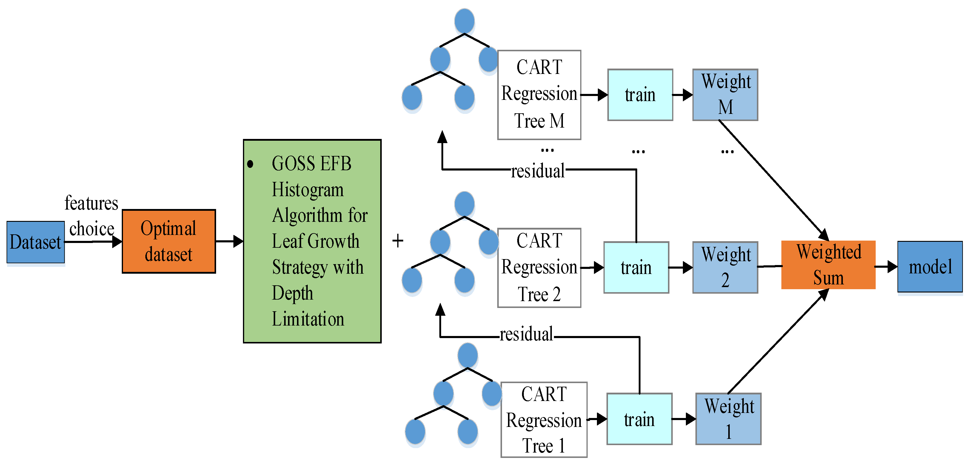
Ensemble learning is a model framework that involves the construction of multiple machine learners, training them to form multiple weak learners and combining them using a specific combination strategy to form a strong learner [20]. LightGBM algorithm represents an implementation of Gradient Boosting Decision Trees (GBDT), characterized by a quicker execution speed and lower vulnerability to overfitting when compared to other enhanced GBDT algorithms. The principle of LightGBM algorithm is shown in Figure 1.
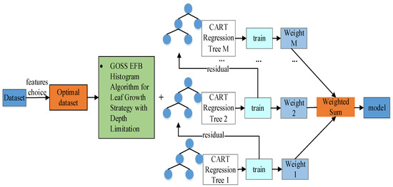
Figure 1.
Schematic of LightGBM algorithm.
LightGBM implements a leaf-wise strategy with depth restrictions to prevent the creation of excessively deep decision trees and mitigate the likelihood of overfitting. It utilizes a histogram algorithm for feature selection and determining segmentation points in decision trees to minimize the quantity of split points. Additionally, LightGBM incorporates GOSS algorithm to filter instances with significant gradients and EFB algorithm to further diminish the number of features.
3. Transformer Fault Diagnosis Model
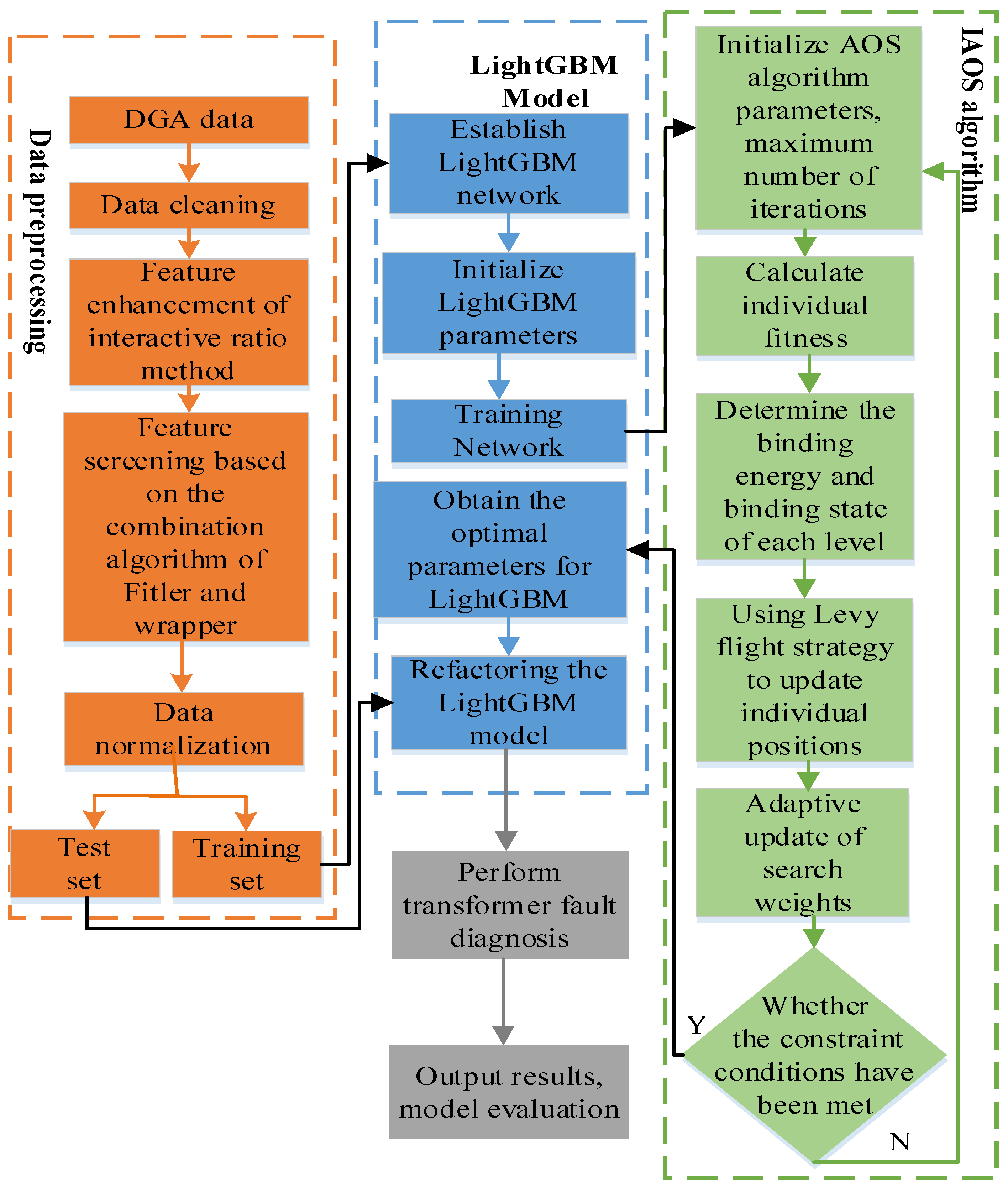
In this study, LightGBM model was employed for transformer fault diagnosis. Given the complexity of LightGBM model with numerous parameters, manual adjustment would be time-consuming and challenging to determine the optimal values. Consequently, the IAOS optimization algorithm was utilized to optimize the parameters of LightGBM model, thereby enhancing the performance of the diagnostic model. An IAOS LightGBM model was developed for transformer fault diagnosis (Figure 2).
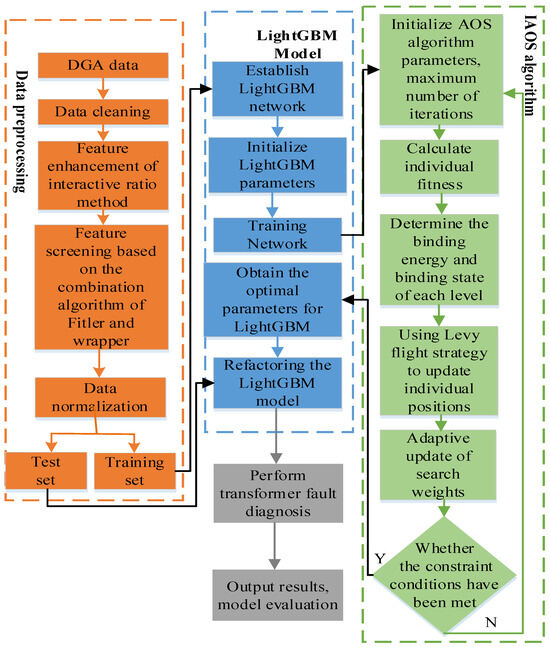
Figure 2.
Transformer fault diagnosis model utilizing IAOS LightGBM.
The transformer fault diagnosis model utilizing IAOS-optimized LightGBM framework is composed of three main components: data preprocessing, IAOS optimization algorithm, and LightGBM model. The implementation steps are outlined as follows:
- A series of data preprocessing steps were performed on DGA sample data, including data cleaning, feature enhancement through the interactive ratio method, feature selection using a combination of Filter and Wrapper algorithms, and normalization;
- The preprocessed data were randomly divided into a training set and a testing set in a specified proportion;
- The hyperparameters of LightGBM model were set to IAOS individuals, and the parameters for both IAOS and LightGBM were initialized;
- The training set was used as input for training, and LightGBM parameters were optimized using IAOS algorithm;
- The model was evaluated with the validation set, and the parameters were adjusted accordingly;
- It was determined whether the training was completed;
- The optimal model was output, the final model was tested with the testing set, diagnostic results were generated, and the model was evaluated.
4. Case Study and Analysis
4.1. Data Acquisition
The data utilized in this study were sourced from a northwest power grid operated by the State Grid Corporation of China. The concentrations of H2, CH4, C2H6, C2H4, and C2H2 were selected as parameters for diagnosing transformer faults, encompassing 381 datasets with identified faults.
The diagnostic model provides the classification of faults present in the transformer. In accordance with the guidelines outlined in GB-T 7252-2016 for Analysis and Determination of Dissolved Gases in Transformer Oil, this study identifies seven fault types for transformer fault diagnosis: low-temperature overheating, medium-temperature overheating, high-temperature overheating, partial discharge, low-energy discharge, high-energy discharge, and normal operation [21]. The dataset was divided into training and testing sets at a ratio of 4:1, with fault state codes and their respective sequence numbers in Table 1.

Table 1.
Classification codes for transformer fault types.
4.2. Data Preprocessing
4.2.1. Data Cleaning
Data cleaning is a crucial step in data processing, involving the correction of incorrect, incomplete, or duplicate data to ensure data quality and availability. In this paper, data cleaning was primarily conducted as follows:
- The missing value is checked and filled with the minimum value; because the subsequent feature engineering needs to perform the feature ratio, if the missing value is filled with 0, 0 as the denominator will produce an abnormal value, so the missing value is filled with a fixed value of 0.01. Some data in the original data are zero, and the feature attributes added by the ratio method have the case that the divisor is zero, so abnormal data will be generated. The processing methods of abnormal data are Pauta criterion and fixed value filling. The DGA data are too scattered and the data level is quite different. The Pauta criterion will eliminate most of the data and the Pauta criterion is not applicable to DGA data. Therefore, the fixed value (0.01) filling method is used to process the abnormal data.
- Outliers are identified and processed to reduce their impact on data feature representation. These outliers are due to abnormal data sensor transmission, resulting in an abnormal data level, which can be replaced by its mean.
- The data type is converted to float for subsequent analysis and processing.
- Duplicate data are identified and removed to avoid errors during analysis and processing.
- Data are uniformly converted to the same numerical range to prevent misunderstandings between data of different specifications.
- Data are integrated into a single dataset, ensuring correct connections between different data points.
- The post-cleaning DGA data are illustrated in Figure 3.
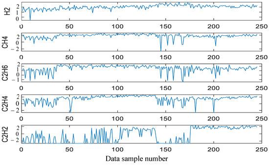 Figure 3. Post−cleaning DGA data.
In Figure 3, the data cleaning process is followed by interpolation of fixed values to solve missing values and outliers in the data set, thereby enhancing data integrity. Because the data of the y-axis are quite different, the above picture has taken the lg value for the y-axis. Data missing value and outlier processing can be divided into two categories: one is to delete missing data and the other is to perform data interpolation. The former is relatively simple and crude, but it may directly affect the objectivity and accuracy of the analysis results. The latter can be completed by means of mean, weighted mean, or median. Here, mean completion is used to improve the accuracy of fault diagnosis.
4.2.2. Feature Enhancement Using Interactive Ratio Method
The coupling phenomenon among the attributes of transformer DGA data leads to notable variations in gas concentration and reduces the diagnostic precision of the results when the raw data are directly utilized as input for the classifier. To address this issue, various methods have been proposed in the literature to enhance diagnostic accuracy. These methods include the three-ratio method (comprising 3-dimensional features), uncoded ratio method (comprising 9-dimensional features), IEC ratio method (comprising 3-dimensional features), and Rogers ratio method (comprising 4-dimensional features). By employing these methods to generate new features, the diagnostic accuracy of the model can be improved [22,23,24].
The feature dimensions produced by the three-ratio method and the uncoded method do not fully disentangle the data. Therefore, this study adopted the ratio method to traverse data attributes to achieve a more effective decoupling.
Ratio method: given that DGA data comprise 5-dimensional attributes, four interactive ratio forms for data attributes were considered: , , , and , where N3, N4, N5, and N6 are different attributes of H2, CH4, C2H6, C2H4, and C2H2 in DGA data; N1 or N2 is any attribute of DGA data (N1 ≠ N2).
The transformer’s dimensions were expanded to 150 by amalgamating 145-dimensional feature variables through the utilization of the aforementioned four ratio forms in conjunction with the original 5-dimensional features.
4.2.3. Feature Selection Using Combined Filter and Wrapper Methods
The inclusion of redundant features may result in multicollinearity issues, while the presence of noisy features can have a detrimental impact on the model, increasing its complexity and potentially leading to overfitting, thereby impacting the diagnostic performance of the model. Feature selection methods such as Filter and Wrapper are frequently employed. In this study, a hybrid approach combining Filter and Wrapper algorithms was utilized for feature extraction, with the following specific process.
The Filter method is primarily utilized for feature selection, involving a specific process outlined as follows: firstly, the mutual information p1 between each feature and the label and the mutual information p2 between features were computed. Features with a mutual information p1 less than 0.05 were irrelevant and likely to lead to model overfitting; thus, features with p1 < 0.05 were eliminated, resulting in the removal of 17-dimensional features. Subsequently, when the mutual information p2 between features exceeded 0.95, indicating high correlation and potential feature redundancy, the feature with the lowest p1 was eliminated from those with p2 < 0.95. This step led to the removal of 78-dimensional features. Overall, 95-dimensional features were eliminated using the Filter method in this study.
Subsequently, the Wrapper method is utilized for feature selection. In this study, a heuristic search is employed, using the IAOS algorithm as the search algorithm and LightGBM model as the classifier. The 45-dimensional features, selected through the Filter method, are binary encoded: elements marked as “1” indicate that the corresponding feature is selected, while elements marked as “0” indicate that the feature is not selected. The resulting features are then used to form a training set, which is divided into training and validation samples using 4-fold cross-validation. LightGBM model is trained with the training samples and the error rate between the predicted values and the actual values of the validation samples is used as the fitness function value. The IAOS algorithm is then employed for optimization, selecting individuals based on their fitness values and ultimately outputting the optimal subset of individuals.
The IAOS algorithm utilized a population size of 50 and 100 iterations to derive a 12-dimensional optimal feature subset. Ultimately, a total of 17-dimensional features were retained, encompassing the original 5-dimensional features.
The features after screening are C2H4/(C2H2 + C2H6), CH4/(H2 + CH4 + C2H4), C2H2/C2H6, H2/(H2 + CH4), C2H2/CH4, H2/C2H6, C2H2/(CH4 + C2H6), C2H2/(H2 + C2H6), C2H2/(H2 + CH4 + C2H6), H2/(C2H2 + C2H6), H2/C2H4, and CH4/(CH4 + C2H6).
4.2.4. Data Normalization
In this study, the interval value method was employed for data normalization. This method scales the data proportionally to a specific interval to mitigate mutual impact among values.
where Xi(d) is the normalized data, with the mapping interval of [−1, 1] (i = 1, 2, …, n); X1 is the original data; max X1 is the maximum value in the data sample; and min X1 is the minimum value in the data sample.
4.3. Transformer Fault Diagnosis Results and Analysis
4.3.1. Fault Diagnosis Based on LightGBM Model
The preprocessed data were partitioned into training and testing sets at a ratio of 4:1. LightGBM model was utilized for transformer fault diagnosis. The classification performance on the testing set is depicted in Figure 4. (The operating environment of the paper is as follows: python3.8, pycharm 2023.1; configuration: Windows 10 standard 64-bit operating system; specific configuration: Intel (R) Core (TM) CPU i9-12900K, 3.2 GHz, 32 GB RAM, and Nvidia Ge-Force GTX 3080 graphics card).

Figure 4.
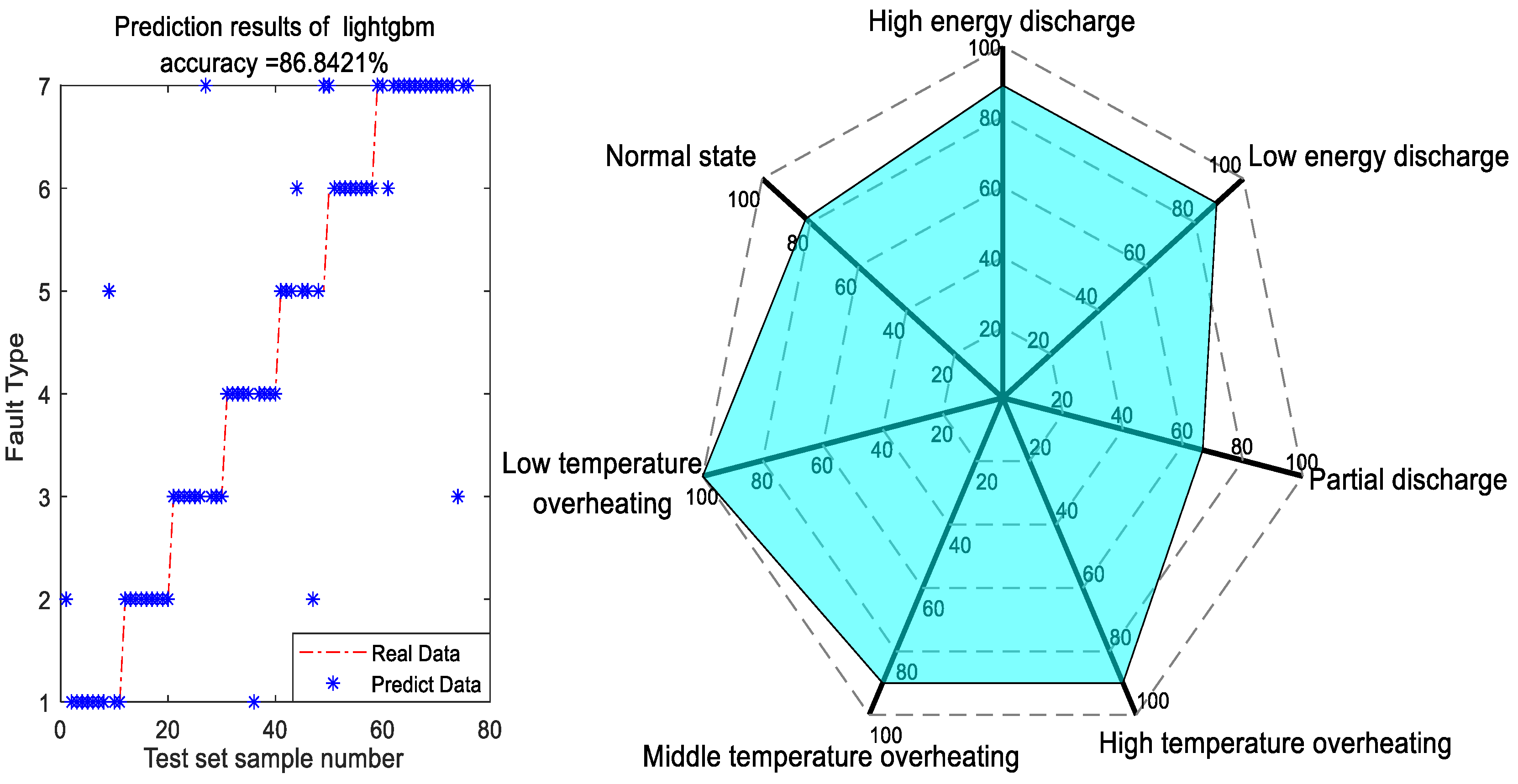
Diagnosis results of LightGBM model.
In Figure 4, LightGBM model is employed for fault diagnosis following feature extraction. The diagnosis effect is the worst in the two categories of normal state and partial discharge, and the diagnosis effect is the best in the high-temperature overheating state and the low-temperature overheating state. The model demonstrated an overall accuracy exceeding 86%, indicating strong performance.
A detailed diagnostic table is as shown in Table 2.
Table 2.
Diagnostic results of LightGBM model under different categories.
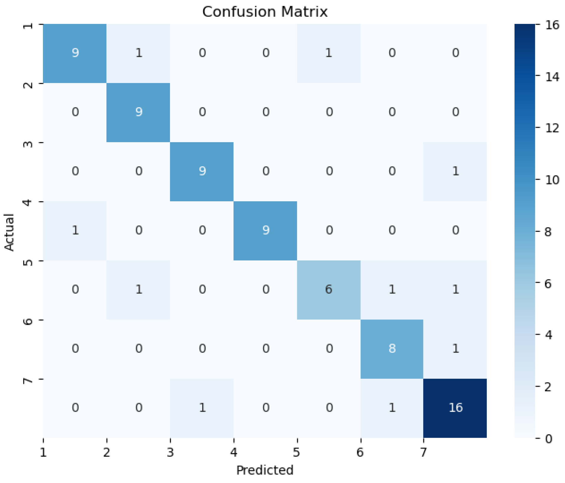
The confusion matrix is shown in Figure 5.

Figure 5.
The confusion matrix of LightGBM model.
4.3.2. Fault Diagnosis Results Using Different Feature Processing Methods
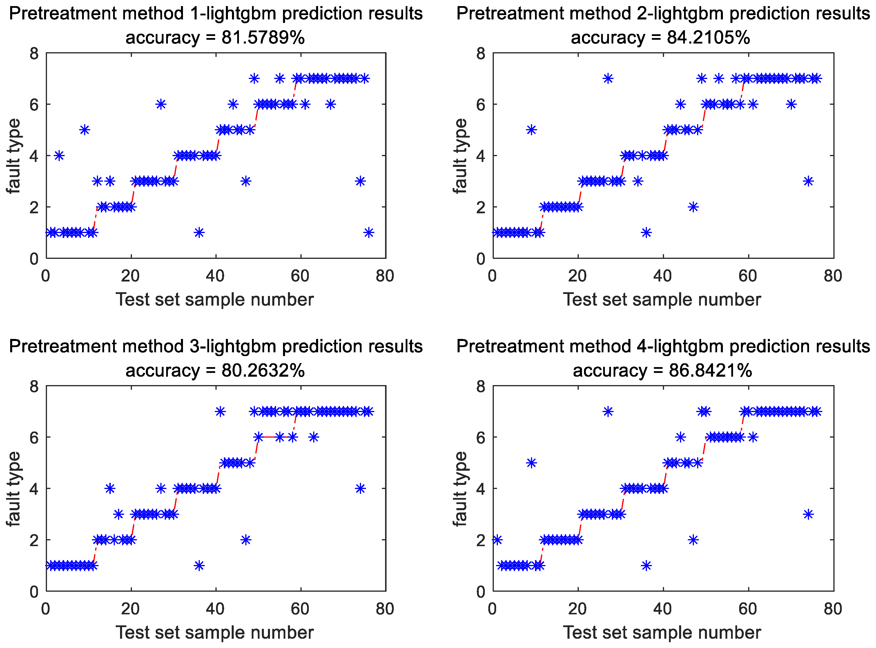
To verify the effectiveness of the proposed feature extraction method, four different feature extraction experiments were conducted as follows:
- Preprocessing method 1: features constructed without the encoding ratio, combined with original features;
- Preprocessing method 2: features constructed using IEC ratio, Rogers ratio, and three-ratio method, combined with original features;
- Preprocessing method 3: raw data without any feature construction;
- Preprocessing method 4: feature extraction method proposed in this paper;
- LightGBM model was employed to classify data processed using four different preprocessing methods, and the diagnostic results of the testing set are illustrated in Figure 6.
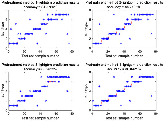 Figure 6. Diagnosis results of LightGBM model using different feature processing methods.
The feature extraction method presented in this study demonstrates the highest accuracy achieving 86.84% (Figure 6). A comparison with the unprocessed raw data reveals a 6.58% enhancement in fault diagnosis accuracy of LightGBM model following the application of the proposed feature extraction method. Figure 6 illustrates that the suggested method exhibits superior accuracy compared to alternative preprocessing techniques under conditions of high-temperature overheating. To ensure result stability, each of the four methods underwent 20 iterations. Statistical analysis was performed on all outputs, and the results are detailed in Table 3.
Table 3.
Fault diagnosis accuracy across different feature processing methods.
In Table 3, various data partitions exhibit a broad spectrum of fluctuations in the testing set accuracy, attributed to substantial variations in the dataset. In contrast to the initial data, the accuracy of transformer diagnosis, as processed by the feature method introduced in this study, demonstrated a 5.62% increase, resulting in an average accuracy of 86.32%.
4.3.3. Impact of Different Optimization Algorithms on Model
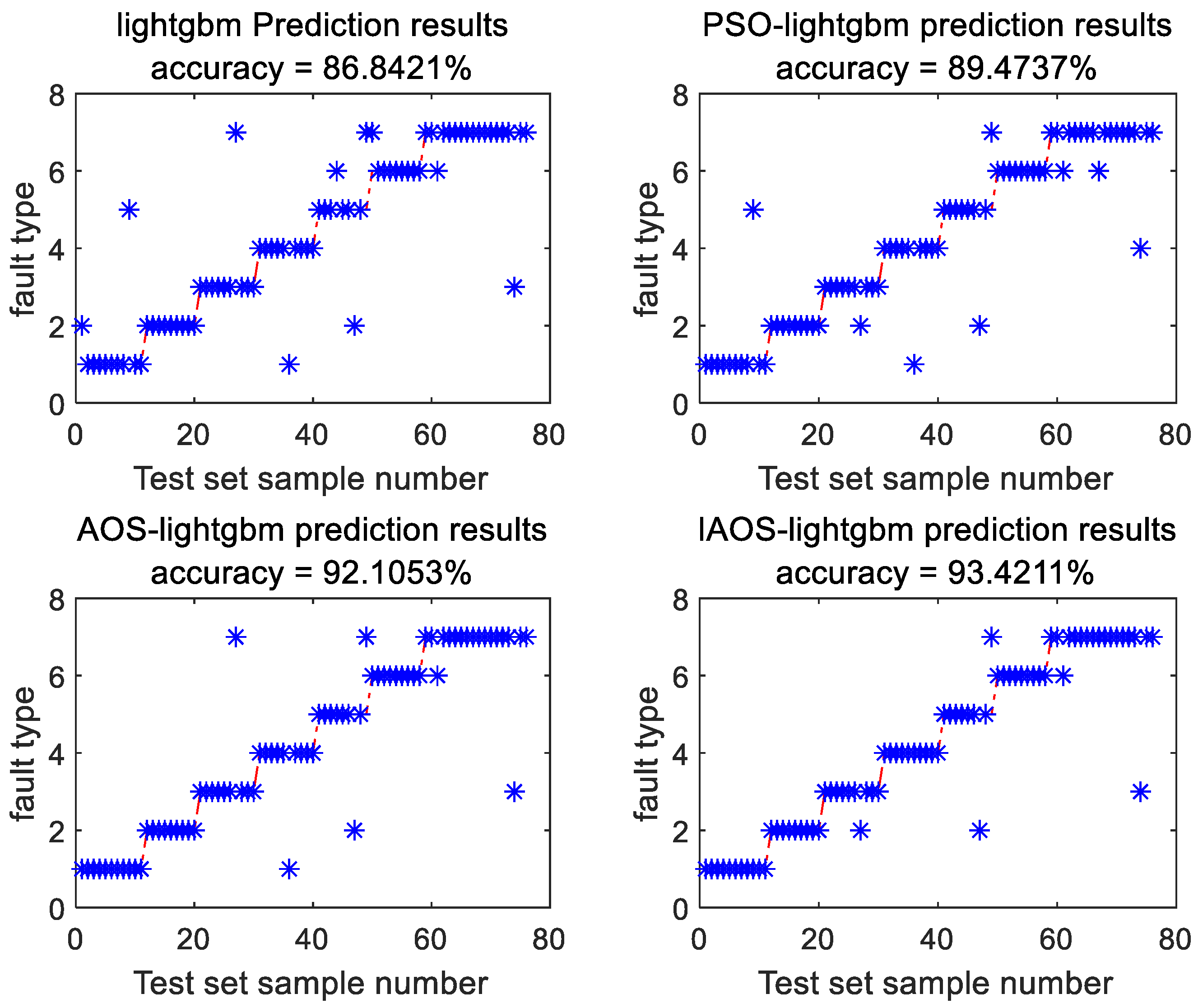
LightGBM model has numerous parameters, many of which significantly impact the model’s accuracy. This study employed the IAOS algorithm, AOS algorithm, and Particle Swarm Optimization (PSO) algorithm to optimize key parameters of LightGBM model, such as the learning rate, regularization parameter, maximum tree depth, number of leaves, iteration count, and min_data_inobun parameter. With a population size of 50 and 100 iterations, the population was partitioned into training and validation samples using a 4-fold cross-validation approach, with the validation set samples serving as fitness values. The trained model was utilized for classifying the testing set, and the results are depicted in Figure 7.
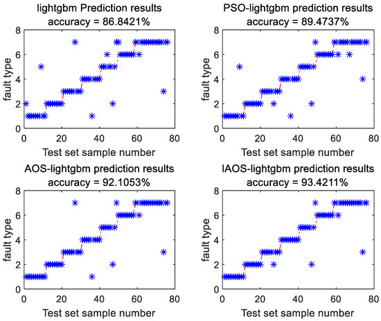
Figure 7.
Diagnosis results using different optimization algorithms.
In Figure 7, the model’s accuracy has shown improvement following the optimization of algorithm parameters. The IAOS–Lightgbm model can accurately identify faults such as low-temperature overheating, medium-temperature overheating, high-temperature overheating, partial discharge, low-energy discharge, and high-energy discharge. Among them, the accuracy of high-temperature overheating identification is the highest, and partial discharge is slightly worse. In the high-temperature overheating category, the IAOS–Lightgbm model has the highest diagnostic effect, with an accuracy rate of 100%. Compared with the Lightgbm model, the accuracy rate is increased by 10%. In the low-energy discharge category, the IAOS–Lightgbm model is 11.11% higher than the Lightgbm model. Specifically, IAOS LightGBM model achieved the highest accuracy of 93.42%, marking a 6.58% increase compared to the unoptimized model and a 1.32% improvement over AOS LightGBM model.
A radar chart was generated for each fault type to enhance the precision of diagnostic accuracy assessment for each fault type (Figure 8). The color of Figure 8 is set to transparency (50%). Some colors in the figure are not on the legend, which is the effect of color mixing on the legend. For example, the mixture of red and yellow will form green.
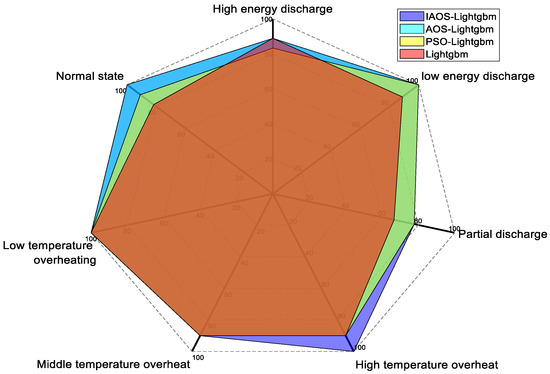
Figure 8.
Accuracy of fault types for each optimization algorithm.
Figure 8 reveals that the accuracy of LightGBM model has significantly increased across all categories following parameter optimization. Notably, this model exhibited superior accuracy compared to other models under high-temperature overheating conditions, while also demonstrating optimal performance in cases of partial discharge. AOS LightGBM model outperformed other techniques in standard operating conditions; however, its accuracy was relatively lower in scenarios involving partial discharge.
5. Conclusions
This paper presented a comprehensive approach to transformer fault diagnosis by processing DGA data through data cleaning, feature enhancement, and feature selection to extract more accurate and comprehensive features. The IAOS-optimized LightGBM model was then applied to classify faults in the processed data, significantly enhancing diagnostic accuracy. The key conclusions are outlined as follows:
- Following preprocessing with the proposed feature extraction method, the data were input into LightGBM model for fault diagnosis, achieving an accuracy of 86.84%, which represents an improvement of 6.58% over the unprocessed data;
- Upon applying the IAOS optimization algorithm for model parameter tuning, the model’s accuracy increased to 93.42%, reflecting a further improvement of 6.58%;
- The IAOS algorithm proposed for parameter optimization enhanced the model’s accuracy by 1.32% compared to the original AOS algorithm.
Outlook:
In this paper, combined Filter and Wrapper methods are used to extract features, and the optimal feature subset is obtained, which improves the diagnosis effect. In the future research, lightweight programs can be used to achieve real-time online diagnostic effects, combined with embedded products to obtain physical products. In the future, to prevent the noise of the collected data, future research work can add Gaussian white noise or use irregular noise to improve the robustness of the model. In terms of feature extraction, after using the ratio method to traverse the features, we can combine the autoencoder to form a semi-supervised model and collect more unlabeled data. The self-supervised model is used to obtain the features and then combined with the diagnostic model to obtain more general features.
Author Contributions
Conceptualization, G.X.; data curation, M.Z.; methodology, G.X.; project administration, M.Z.; resources, M.Z. and G.X.; validation, G.X.; visualization, W.C. and Z.W.; writing—original draft, G.X. and Z.W.; writing—review and editing, G.X. and W.C. All authors have read and agreed to the published version of the manuscript.
Funding
This research was funded by National Natural Science Foundation of China (52374154).
Institutional Review Board Statement
Not applicable.
Informed Consent Statement
Not applicable.
Data Availability Statement
Data are available upon request.
Conflicts of Interest
Author Wanli Chen was employed by the State Grid Jingning County Power Supply Company. The remaining authors declare that the research was conducted in the absence of any commercial or financial relationships that could be construed as a potential conflict of interest.
References
- Xie, G.M.; Wangm, J.L. Transformer fault identification method based on hybrid sampling and IHBA-SVM. J. Electr. Measur. Instrument. 2022, 36, 77–85. [Google Scholar]
- Yang, L.; Gao, L.; Luo, X.; Hao, Y.; Zhang, Z.; Jin, Y.; Zhang, J. An Improved Method for Fault Diagnosis of Oil-Immersed Transformers Based on Simulation Test Platform. IEEE Trans. Dielectr. Electr. Insul. 2024. [Google Scholar] [CrossRef]
- Taha, B.I.; Mansour, A.D. Novel Power Transformer Fault Diagnosis Using Optimized Machine Learning Methods. Intell. Autom. Soft Comp. 2021, 28, 739–752. [Google Scholar] [CrossRef]
- Chen, T.; Chen, W.D.; Li, X.S.; Chen, Z. Transformer fault prediction based on analysis of dissolved gas in oil. Electr. Measur. Technol. 2021, 44, 25–31. [Google Scholar]
- Kirkbas, A.; Demircali, A.; Koroglu, S.; Kizilkaya, A. Fault diagnosis of oil-immersed power transformers using common vector approach. Electr. Power Syst. Res. 2020, 184, 106346. [Google Scholar] [CrossRef]
- Qu, Y.H.; Zhao, H.S.; Ma, L.B.; Zhao, S.C.; Mi, Z.Q. Multi-Depth Neural Network Synthesis Method for Power Transformer Fault Identification. Chin. Soc. Electr. Eng. 2021, 41, 8223–8231. [Google Scholar]
- Jiang, Y.J.; Tang, X.F.; Tang, D.C.; Zhao, M.Y.; Jing, B.Q. A transformer fault prediction method based on the fusion of grey theory and IEC triple ratio. J. Guilin Univ. Aerosp. Technol. 2024, 29, 38–45. [Google Scholar]
- Hoballah, A.; Mansour, D.E.A.; Taha, I.B.M. Hybrid grey wolf optimizer for transformer fault diagnosis using dissolved gases considering uncertainty in measurements. IEEE Access 2020, 8, 139176–139187. [Google Scholar] [CrossRef]
- Yang, X.; Chen, W.; Li, A.; Yang, C.; Xie, Z.; Dong, H. BA-PNN-based methods for power transformer fault diagnosis. Adv. Eng. Inform. 2019, 39, 178–185. [Google Scholar] [CrossRef]
- Yan, C.; Li, M.; Liu, W. Transformer fault diagnosis based on BP-Adaboost and PNN series connection. Math. Probl. Eng. 2019, 9, 1019845. [Google Scholar] [CrossRef]
- Wu, G.; Yao, J.; Guan, M.; Zhu, X.; Wu, K.; Li, H.; Song, S. Power transformer fault diagnosis based on DBSCAN. J. Wuhan Univ. 2021, 54, 1172–1179. [Google Scholar]
- An, G.; Shi, Z.; Ma, S.; Han, X.; Du, Z.; Zhao, C. Woa-svm transformer fault diagnosis based on RF feature optimization. High Volt. Appar. 2022, 58, 171–178. [Google Scholar]
- Rao, S.; Zou, G.; Yang, S.; Barmada, S. A feature selection and ensemble learning based methodology for transformer fault diagnosis. Appl. Soft Comput. 2024, 150, 111072. [Google Scholar] [CrossRef]
- Zhang, Y.W.; Feng, B.; Chen, Y.; Liao, W.H.; Guo, C.X. Fault diagnosis method for oil-immersed transformer based on XGBoost optimized by genetic algorithm. Electr. Power Autom. Equip. 2021, 41, 200–206. [Google Scholar]
- Wang, Y.H.; Wang, Z.Z. Transformer fault identification method based on RFRFE and ISSA-XGBoost. J. Electr. Measur. Instrum. 2021, 35, 142–150. [Google Scholar]
- Zhang, M.; Chen, W.; Zhang, Y.; Liu, F.; Yu, D.; Zhang, C.; Gao, L. Fault diagnosis of oil-immersed power transformer based on difference-mutation brain storm optimized Catboost model. IEEE Access 2021, 9, 168767–168782. [Google Scholar] [CrossRef]
- Hu, L.Y.; Jiang, W.B.; Li, Y.T. Fault diagnosis for wind turbine based on lightgbm. Acta Energiae Solaris Sin. 2021, 42, 255–259. [Google Scholar]
- Xu, B.Q.; He, J.C.; Sun, L.L. Fault detection method of cage asynchronous motor based on stacked autoencoder and improved LightGBM algorithm. Electr. Mach. Control 2021, 25, 29–36. [Google Scholar]
- Azizi, M. Atomic orbital search: A novel metaheuristic algorithm. Appl. Math. Model. 2021, 93, 657–683. [Google Scholar] [CrossRef]
- Han, X.; Wang, X.Y.; Han, S.; Zhang, Y.T.; Wang, J.Y. Ensemble learning method for large-scale power transformer status evaluation based on imbalanced data. Power Syst. Technol. 2021, 47, 107–114. [Google Scholar]
- GB-T 7252-2016; Guidelines for Analysis and Determination of Dissolved Gases in Transformer Oil. China Standard Press: Beijing, China, 2016.
- Yu, S.; Hu, D.; Tang, C.; Zhang, C.M.; Tan, W.M. MSSA-SVM transformer fault diagnosis method based on TLR-ADASYN balanced data set. High Volt. Eng. 2021, 47, 3845–3853. [Google Scholar]
- Liu, Z.; He, W.; Liu, H.; Luo, L.; Zhang, D.; Niu, B. Fault identification for power transformer based on dissolved gas in oil data using sparse convolutional neural networks. IET Gener. Transm. Distrib. 2023, 18, 517–529. [Google Scholar] [CrossRef]
- Gong, Z.W.Y.; Rao, T.; Wang, G.; Li, Z.; Luo, Z.; Zhu, J.X.; Peng, J.; Yu, H.; Cao, Z.G. Fault diagnosis method of transformer based on improved particle swarm optimization XGBoost. High Volt. Appar. 2023, 59, 61–69. [Google Scholar]


Disclaimer/Publisher’s Note: The statements, opinions and data contained in all publications are solely those of the individual author(s) and contributor(s) and not of MDPI and/or the editor(s). MDPI and/or the editor(s) disclaim responsibility for any injury to people or property resulting from any ideas, methods, instructions or products referred to in the content. |
© 2024 by the authors. Licensee MDPI, Basel, Switzerland. This article is an open access article distributed under the terms and conditions of the Creative Commons Attribution (CC BY) license (https://creativecommons.org/licenses/by/4.0/).