Article

High-Performance Mobility Simulation: Implementation of a Parallel Distributed Message-Passing Algorithm for MATSim †

Transport Systems Planning and Transport Telematics, Institute of Land and Sea Transport Systems, Technische Universität Berlin, Kaiserin-Augusta-Allee 104-106, 10365 Berlin, Germany
*
Author to whom correspondence should be addressed.
This article is a revised and expanded version of a conference paper entitled High-Performance Simulations for Urban Planning: Implementing Parallel Distributed Multi-Agent Systems in MATSim, which was presented at the 23rd International Symposium on Parallel and Distributed Computing (ISPDC), Chur, Switzerland, 8–10 July 2024.
Information 2025, 16(2), 116; https://doi.org/10.3390/info16020116
Submission received: 25 December 2024 / Revised: 27 January 2025 / Accepted: 5 February 2025 / Published: 7 February 2025

Abstract

:
Striving for better simulation results, transport planners want to simulate larger domains with increased levels of detail. Achieving fast execution times for these complex traffic simulations requires the parallel computing power of modern hardware. This paper presents an architectural update to the MATSim traffic simulation framework, introducing a prototype that adapts the existing traffic flow model to a distributed parallel algorithm. The prototype is capable of scaling across multiple compute nodes, utilizing the parallel computing power of modern hardware. Benchmarking reveals a 119-fold improvement in execution speed over the current implementation, and a 43 times speedup when compared to single-core performance. The prototype can simulate 24 h of large-scale traffic in just 3.5 s. Based on these results, we advocate for integrating a distributed simulation approach into MATSim and outline steps for further optimizing the prototype for large-scale applications.

1. Introduction

Shaping the future of growing metropolitan areas [1] requires careful planning of the transportation infrastructure. Traffic simulations are an essential tool for city planners to evaluate traffic management policies [2] and infrastructure changes [3]. As traffic simulation models continue to evolve, there is a growing demand to enhance their scale and level of detail, significantly increasing the computational requirements of such software [4]. At the same time, CPU (Central Processing Unit) clock rates have plateaued for nearly two decades, and the miniaturization in semiconductor design is approaching physical limits [5]. Realizing performance improvements to accommodate computationally expensive simulations while maintaining fast execution times requires leveraging the parallel computing capabilities of modern computer hardware.

1.1. Motivation

MATSim (Multi-Agent Transport Simulation) [6] v15.0 is a well established software framework for agent-based traffic modelling. Operating on a mesoscopic scale, it supports simulating urban regions encompassing millions of individual travelers. Traffic in MATSim is modelled using synthetic persons which travel along a simulated road network to reach designated activity locations. Over multiple iterations of the same simulated day, synthetic persons explore various strategies to maximize their utility. One iteration consists of three phases: (1) the mobsim (mobility simulation) phase, where synthetic persons execute their daily plans; (2) the scoring phase, where executed plans are evaluated; and (3) the replanning phase, where a fraction of the synthetic population invents new plans to test during the next iteration.
Among the three phases outlined above, phases 2 and 3 are embarrassingly parallel problems. In contrast, distributing the mobsim phase onto parallel computing hardware is more challenging, as synthetic persons interact while travelling within the simulation. Therefore, when developing a new parallel architecture for MATSim we focus on the mobsim phase, assuming that phase 2 and 3 can be integrated later.
The default implementation of the mobsim, QSim, already facilitates multicore systems using Java’s concurrency primitives and a shared memory algorithm [7]. This approach effectively scales up to 8 processes. Executing the mobsim with more processes does not improve execution times, possibly limited by transfer rates between memory and the CPU [8].
Modern hardware supports significantly more processors, requiring a new parallelization strategy. We propose switching to a message-passing approach [9], which explicitly models data exchange between computing processes. This approach is particularly well-suited for distributed computing environments, such as HPC (High-Performance Computing) clusters, where each physical machine handles a specific portion of the computational problem. By distributing the workload across multiple computing nodes, the amount of data transferred through the memory bus on each node is reduced, as each process manages only its assigned share of the computation. Furthermore, with each process responsible for a fraction of the traffic simulation, cache locality can be improved, leading to faster execution times on multicore machines.

1.2. Aim of the Study

In this study, we present an architectural update to MATSim’s default mobsim implementation, QSim by applying the message passing concept for parallelization from our previous work [9].
  • We develop a prototype implementation that scales on HPC clusters. The implementation is fully compatible with MATSim’s input and output format, allowing the use of existing and calibrated simulation scenarios for testing. The prototype implementation is available as an open-source GitHub repository (https://github.com/matsim-vsp/parallel_qsim_rust, accessed on 4 February 2025) and release v0.2.0, used in this study, is captured as a Zenodo repository [10].
  • We benchmark the prototype on the HRN@ZIB HPC cluster, capable of scaling to more than one thousand processes, using an open-source, real-world simulation scenario. Similar to the source code, all input, and output files are available under an open-access license in a Zenodo repository to enable reproducibility [11].
  • Based on the executed benchmarks, we show that the distributed algorithm is latency bound even on high-performance communication hardware, and that balancing the computational load becomes less of a problem for large numbers of computing processes at the cost of computational efficiency. Additionally, we can show that the time dedicated to inter process communication depends on the maximum number of neighbors any process has.
This study extends our previous work [9] by adapting the original message-passing algorithm to the current MATSim framework. In our earlier work, we proposed the concept of message-passing parallelization and speculated that achievable speedups might be constrained by communication hardware latency. Using modern HPC infrastructure, we confirm that this latency limit persists even with advanced, low-latency hardware. Unlike the previous study, we profile performance at the time-step level, offering detailed insights into where computational time is spent. These detailed performance metrics provide a new level of granularity, which was not addressed in the earlier work. We also evaluate benchmarks with varying sample sizes to investigate how problem size impacts speedup and execution time, demonstrating a more comprehensive understanding of computational scalability.
In addition to these improvements, this study extends a conference paper [12] that introduced the prototype implementation. Based on feedback received at the conference, we have significantly refined the description of the implemented algorithm, improving its reproducibility. Furthermore, we expanded the benchmarks by including varying computational loads to compare speedups under different conditions. We also add a detailed comparison to other parallel traffic simulation implementations, positioning our approach within the research landscape. Together, these enhancements make this study a substantial progression over both our previous conceptual work and the preliminary conference presentation.

1.3. Related Work

Efforts to accelerate MATSim include the Hermes project [8], which implemented a mobsim optimized for single-core performance. Alternatively, Strippgen [13] developed a mobsim designed for GPU (Graphics Processing Unit) hardware, enabling massive parallelism. However, integrating their solution into the broader MATSim framework proved challenging. More recently, Wan et al. [14] introduced a distributed version of MATSim, achieving its fastest execution times with four processes and a speedup of two—significantly less than the performance of the parallelization strategy presented in this study.
Beyond the MATSim ecosystem, parallel traffic simulations have utilized multicore hardware with mixed results. Gong et al. [15] employed OpenMP [16] to develop an agent-based model tested on up to 32 processes. Similarly, Qu and Zhou [17] implemented a queue-based simulation using OpenMP, which scaled effectively up to 10 CPU cores. Bragard et al. [18] investigated online load-balancing in microscopic traffic simulations, testing their approach across four computing nodes. Mobiliti, introduced by Chan et al. [19], is a discrete event simulation independent of MATSim that uses optimistic synchronization methods and scales well on HPC infrastructure. We include a detailed comparison of Mobiliti in the discussion section (see Section 4.5).
Recent advances in GPU technology have also spurred interest in accelerating traffic simulations with hardware accelerators [20]. For instance, the activity-based demand model by Zhou et al. [21] achieves a 50-fold speedup compared to single-core implementations. The GEMSim project [22,23] implements a queue-based traffic simulation supporting public transit and claims a ninefold improvement over state-of-the-art tools.

2. Methodology

We find in our previous work that the runtime of the proposed algorithm is constrained by the latency of message exchanges [9]. This indicates that a new implementation should support low-latency networking hardware, such as Infiniband (manufactured by Nvidia, Santa Clara, CA, USA), or OmniPath (manufactured by Intel, Santa Clara, CA, USA). The conventional high-level abstraction to utilize this hardware is MPI (Message Passing Interface) [24], which Java – the programming language for MATSim – does not natively support. Attempts to run a Java setup with available libraries, such as Open MPI v4.1.2 [25,26], were unsuccessful on several combinations of hardware and operating systems. Executing a Java process within an MPI context resulted in crashes of the JVM (Java Virtual Machine) caused by SIGSEGV signals and could not be resolved using the Open MPI mailing list or the Open MPI issue tracker (https://github.com/open-MPI/oMPI/issues/10223, accessed on 6 February 2024). Consequently, we opted to develop a prototype in Rust, which allows direct interfacing with the C implementation of Open MPI. The prototype implementation is available as open-source code on GitHub (https://github.com/matsim-vsp/parallel_qsim_rust, accessed on 6 February 2024) and this paper is based on v0.2.0 [10].
The prototype implementation maintains compatibility with the most important input and output files of the current MATSim implementation. By using the existing MATSim input formats, it enables the utilization of existing simulation scenarios to test the implemented prototype. Additionally, the prototype produces an event log identical to that of the current mobsim implementation, capturing events such as activities starting and ending, or vehicles entering and leaving network links. During the execution of the distributed mobsim prototype, each process generates an individual events file, which can be merged after the simulation has finished. The produced events file can be analyzed using the software already available for the existing MATSim framework, allowing the simulation results of the prototype implementation to be easily verified.

2.1. Traffic Flow Simulation

The traffic simulation executed in each process is similar to MATSim’s current QSim implementation, as described by Horni et al. [6] (Chapter 1). We will outline the core concepts of the implemented algorithm for the prototype and highlight differences to the Qsim at the end of this section.
The traffic flow simulation operates on a directed graph that simulates a road network. Nodes represent intersections where vehicles change links, while links model street segments. Each link carries information necessary to calculate the traffic flow, including freespeed (the maximum speed under free flow conditions), storage capacity (the maximum number of vehicles under congestion), and flow capacity (the limit on vehicles traversing a link per time period). Agents travel between activities along pre-planned routes comprised of a sequence of links.
The simulation uses an intersection-oriented algorithm. During updates, vehicles at the end of incoming links are considered for movement across intersections. In Figure 1 the two vehicles at the end of the links which point to the node in the center would be considered. Whether a vehicle can be moved over an intersection depends on storage and flow capacity constraints, described next, followed by an explanation of the intersection update process.

2.1.1. Link Management

Traversing a link includes three phases:
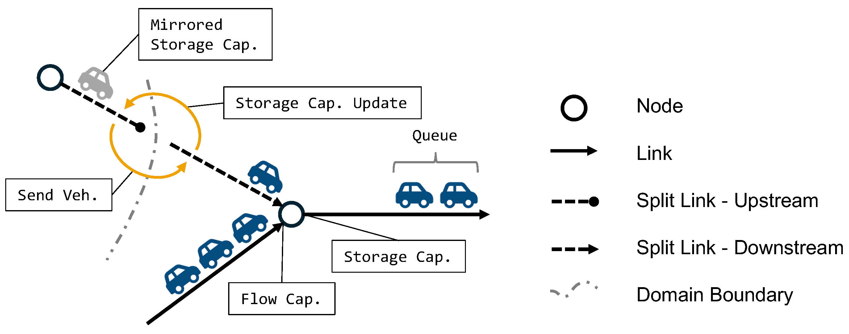
  • Entering the link: Vehicles can enter a link only if sufficient storage capacity is available. The storage capacity of a link is determined by its length and number of lanes. For example, assuming one car occupies 7.5 m, a 30 m one lane link has a capacity of 4 cars. Figure 1 illustrates this constraint at the start of the link.
  • Traversing the link: Vehicles traversing the link are managed using a queue. In the example of Figure 1 two vehicles are managed in the queue of the link on the right. The prototype implements a FIFO (First In First Out) queue so that vehicles leave in the same order as they have entered a link. The earliest exit time by which a vehicle can exit a link under free flow conditions is determined by the freespeed of the link (one can consider this to be the street’s speed limit), and the vehicle’s maximum velocity. Vehicles stay in the queue at least until the simulation reaches the calculated earliest exit time. The FIFO characteristics also mean, that if a vehicle is blocked by another vehicle, it cannot leave the link upon its earliest exit time, but has to wait until all other vehicles in front of it have left the link. One reason for a vehicle blocking other vehicles behind it can be a lower maximum velocity. Faster vehicles have to queue behind that vehicle.
  • Leaving the link: The vehicle at the head of the queue may leave the link if the simulation has progressed to its earliest exit time. To actually leave the link, a second condition, sufficient flow capacity, must be met. The flow capacity determines how many vehicles can traverse a link within a given time period. On a residential road, for example, the flow capacity can be assumed to be 600 vehicles per hour. This translates to one vehicle every six seconds. With the help of Figure 1 we can explain how this constraint is enforced. We assume that all three vehicles queued on the link on the left have the same earliest exit time, while the link has a capacity of 600 vehicles per hour. When the simulation reaches the earliest exit time of the vehicles, the first vehicle would be able to leave the link immediately—given that the next link has sufficient storage capacity. The second vehicle would also be able to leave, given its earliest exit time. However, as the first vehicle has consumed one unit of flow capacity, the second vehicle has to wait another six seconds before enough flow capacity has accumulated on the link, for it to exit. Figure 1 illustrates that the flow capacity constraint is enforced at the end of the link by pointing the label to the end of the incoming link.
This queuing mechanism simplifies the traffic dynamics calculation, so that only the earliest exit time of the first vehicle in the queue must be checked during intersection updates, making it computationally very efficient. Although this approach does not model vehicle dynamics such as acceleration or following behavior, it effectively simulates congestion and spill back effects on a saturated road network.

2.1.2. Intersection Update

For the intersection update which moves vehicles from one link to the next, all nodes contained in a network partition are iterated in each time step. Incoming links are handled in random order, weighted by their capacity. Listing 1 shows the intersection update implemented for the prototype for one node in the network. Initially, the algorithm sums up the flow capacities of all incoming links and then moves vehicles over the intersection until all flow capacities are exhausted. As the first step of the intersection update, a random incoming link is selected. The random selection is weighted by flow capacity, so that links with higher flow capacities are more likely to be selected. For a vehicle to move over the intersection, three conditions must be met: (1) the link’s flow capacity is not exhausted, (2) the first vehicle in the queue can leave because the simulation time has advanced to its earliest exit time, and (3) the next link in the vehicle’s route has storage capacity available. In case all conditions are met, the vehicle is removed from the link’s queue and placed onto the next link in the vehicle’s route. The available flow capacity is reduced by the flow capacity consumed by the vehicle which crossed the intersection, and the update loop is continued according to Line 23. If the link cannot emit a vehicle as none of the conditions is met, the link is exhausted because all vehicles on that link are blocked by the first vehicle. The total flow capacity is reduced by the remaining flow capacity of the exhausted link and the link is removed from the choice set of active links (Lines 27, 28), before the update loop continues.
Additionally, the intersection update handles the termination of vehicles that complete their route. To keep the code example in Listing 1 simple, this termination logic is omitted. When a vehicle is selected to leave the last link of its route during the intersection update, the code checks whether it has more links to traverse during its current leg, as shown in Line 15 of Listing 1. Vehicles that have completed their route are removed from the simulated network, and their drivers are added to the simulation’s activity queue after updating their state accordingly.
The traffic flow simulation implemented for the prototype is oriented toward MATSim’s current QSim implementation, with some distinctions:
  • In the QSim, links are split into two segments: a queue and a buffer. Vehicles entering a link from an intersection are first placed in the queue, similar to our approach. However, when a vehicle becomes eligible to exit the link (based on its exit time), given sufficient flow capacity, it is placed into the buffer of the link. During the intersection update, only vehicles in a link’s buffer are considered for crossing the intersection. This separation of queue and buffer is primarily necessary in QSim due to its use of data structures shared between concurrent threads. By splitting the link into these two parts, QSim allows independent operations at the upstream and downstream ends of a link in parallelized executions. In contrast, our prototype relies on a message-passing approach, ensuring that each process operates on its data in isolation. This eliminates the need for an additional buffer data structure, as the flow capacity constraint is enforced directly within the queue.
  • Because links in the prototype implementation only manage a single queue data structure, the flow capacity constraint is enforced during the intersection update. In contrast, the QSim enforces this constraint when vehicles are moved from the queue to the buffer of a link.
  • The QSim calculates the available storage capacity based on the vehicles present in the queue. Since the intersection update in the QSim only operates on vehicles in the link’s buffer, changes to the storage capacity are propagated to the upstream end of the link in the next time step. In the prototype implementation, which operates on a single queue data structure, this behavior is emulated using a bookkeeping mechanism. This mechanism releases storage capacity for vehicles leaving a link only after the intersection update for all nodes within a network partition is completed.
  • Another key distinction is how vehicles are handled upon entering and exiting traffic. In our implementation, vehicles are added to the end of the queue when they enter traffic, and they fully traverse the last link of their route before being removed during the intersection update. This approach allows the termination of vehicles to be handled as part of the intersection update, as previously described. In contrast, MATSim’s QSim inserts and removes vehicles between the queue and the buffer.
Listing 1. Intersection Update.
Information 16 00116 i001

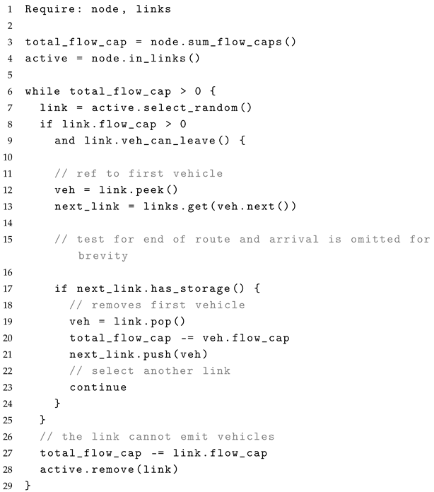
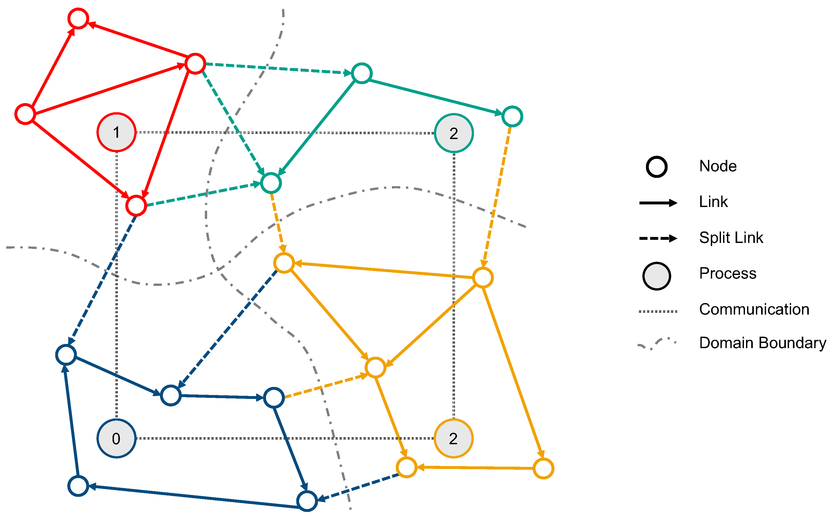
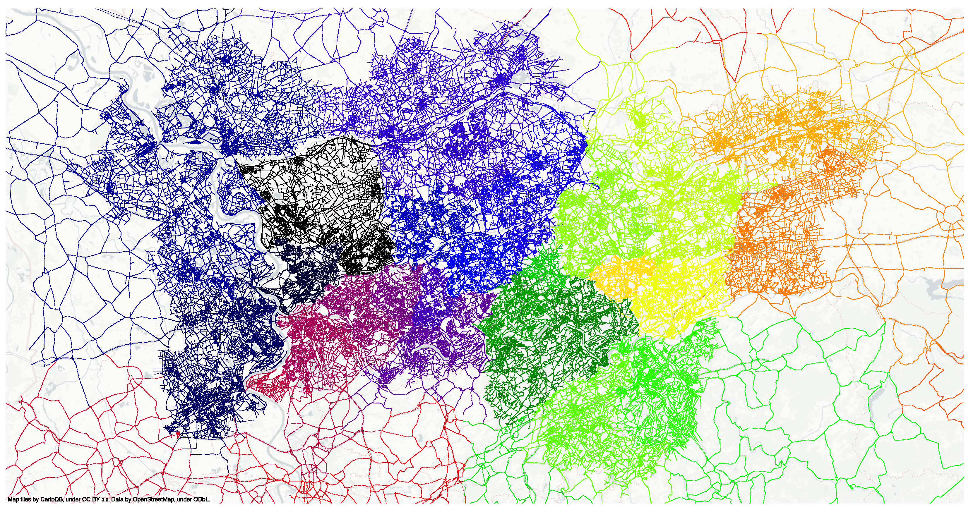
2.2. Domain Decomposition

The proposed algorithm by Cetin et al. [9] employs domain decomposition of the network graph to distribute the simulation workload across processes. Multiple processes may be executed in parallel on the same multicore machine, or each process can be run on a separate machine. In most HPC setups, a combination is used, with multiple machines executing several processes each. Each process is responsible for one domain derived from the domain decomposition phase, performing a single threaded traffic simulation for the network segment within its domain. Vehicles crossing a domain boundary are transmitted as messages to the corresponding other process. Likewise, information on available storage capacities (i.e., if the downstream link has space to accommodate an incoming vehicle) is communicated to neighbor processes. Messages are exchanged between neighboring domains once per simulated time step, consolidating all vehicle crossings and capacity updates into a single message per neighboring process.
The diagram in Figure 2 illustrates how nodes and links of the traffic network are distributed across subdomains. In the example, the network is divided into four partitions, each assigned to corresponding processes. Process 0 has process 1 and 3 as direct neighbors. Their neighbor relationship is established by the shared links, displayed as dashed arrows. To explain how links are shared between processes, we focus on the link shared between process 0 and process 1. Shared links are divided into two parts: an upstream and a downstream part. Since the link in focus points toward a node located in process 0, the downstream part is assigned to process 0, while the upstream part is maintained by process 1. Figure 1 provides a more detailed view of a split link. The downstream part includes the representation of the link, managing the vehicle queue. In the case shown in Figure 1, the downstream part contains one vehicle in its queue. The upstream part mirrors the occupied storage capacity, as indicated by the gray vehicle. Changes in storage capacity, due to vehicles leaving the downstream part, are communicated to the upstream part in the form of a message. The upstream part is connected to the node located on the upstream process, allowing it to receive vehicles during the upstream process’s intersection update. With knowledge of the blocked storage capacity, the upstream process can independently perform an intersection update, placing vehicles on the upstream part. When vehicles enter the split link during this update, they are sent to the downstream part as a message, where they are added to the downstream part’s queue.
Domain decomposition is performed using the METIS library [27], with the option to assign node weights that reflect the anticipated computational load for each network node. METIS balances the node-weights across different network partitions. For the presented results, the computational load for each network node is estimated by parsing all plans of the synthetic population and counting the number of vehicles crossing each node. This way, the computational load is balanced over the simulated day, but may vary for particular time steps in the simulation. As the domain decomposition is node-based, all links pointing toward a node are assigned to the same network partition as the node.

2.3. Simulation Loop

Based on the partitioned network graph and before running the actual simulation loop, each process loads its portion of the network along with all synthetic persons performing their first activity within its domain. The isolation of processes—interacting only through message exchanges—simplifies the implementation by eliminating the need for managing parallel access to data structures. The simulation work is executed on each process following Listing 2. For each time step in the simulation, the following algorithmic steps are performed:
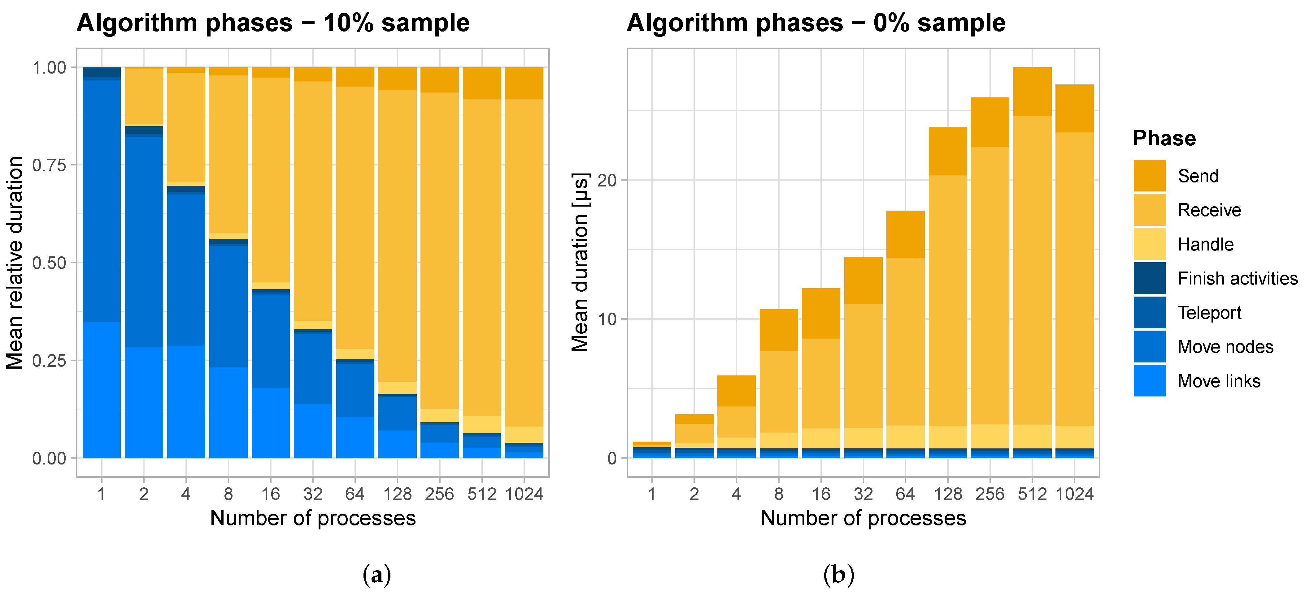
  • Finish activities: Synthetic persons performing activities are stored in a priority queue, ordered by the end time of their activities. Those who have reached the end time of an activity are removed from the queue and start the next plan element, which involves either a teleportation leg or a leg performed on the simulated network.
  • Teleport: Synthetic persons finishing a teleportation leg start the next activity by being placed into the activity queue (see [28] (Chapters 12.3.1, 12.3.2) for the concept of teleported legs).
  • Move nodes: This step corresponds to the intersection update explained in Section 2.1 and involves iterating over all nodes of the network partition, moving vehicles that have reached the end of a link onto the next link in the vehicle’s route. In the case of a vehicle reaching the end of its route, the vehicle is removed from the simulated network and the next plan element of the synthetic person is started by placing it into the activity queue.
  • Move links: The movement of vehicles on the network is constrained by the flow and storage capacities of links. During the move links step, the bookkeeping of these capacities is updated for the next time step. This step also includes collecting all vehicles and capacity updates that must be sent to another process.
  • Send and receive The collected vehicles and capacity updates are passed to a message broker, which coordinates the message exchange with other processes. This step involves communicating the collected information to the corresponding processes, as well as awaiting and receiving incoming messages (see Section 2.4). Received vehicles and capacity updates from other processes are applied to the simulated network in this step.
Steps 1 to 4 perform the simulation work for one process. Step 5 does not perform any simulation work, but is only concerned with inter process communication.
Listing 2. Main simulation loop.
Information 16 00116 i002

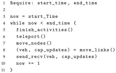
2.4. Inter Process Communication

The message exchange between processes is managed by a message broker component, which oversees the MPI-context. This component maintains a mapping of links to processes, enabling it to identify which process manages each link. Vehicles and capacity updates collected from Step 4 in Section 2.3 are forwarded to the message broker. The broker determines the destination process for each vehicle by checking the target link ID against the link-to-process mapping. Similarly, for capacity updates, the broker looks up the process responsible for the mirror link to which the updated capacity must be communicated. Vehicles and capacity updates are then encapsulated into messages, with each message designated for a specific neighbor process. To reduce the number of messages exchanged, a single message is sent between two processes, which consolidates all update information from one process to the other. Once all messages are prepared, the message exchange proceeds as outlined in Listing 3. The algorithm has three main steps:
  • Send: Corresponding to lines 4–6 this step involves serializing messages into the wire format and issuing a non-blocking ISend call to the underlying MPI implementation for each neighbor process.
  • Receive: On line 12 a blocking Recv call to the underlying MPI implementation is issued and the process awaits messages from any other process. This step is the rendezvous point for neighbors, as faster processes must wait for slower processes to send messages, before they can be received. Additionally, this step involves the time to transmit messages over the communication hardware.
  • Handle: On lines 13–14, received messages are deserialized from wire format back into a message data structure and pushed into the result list.
Listing 3. Inter process communication.
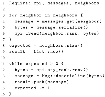
Information 16 00116 i003
The receive step of the algorithm (line 12, Listing 3) is critical as it involves both synchronization and communication between processes, which significantly impact the overall runtime of the simulation. Figure 3 schematically displays the message exchange between two processes. Before exchanging messages, both processes perform their share of the traffic simulation computation, indicated by blue arrows. The blue arrows correspond to Steps 1 to 4 described in Section 2.3. Since the computational load is not perfectly balanced, Process 2 finishes the computation for the current simulation time step first. It then enters the communication phase of the algorithm, represented by yellow arrows, and issues the ISend call on line 6 in Listing 3. As this is a non-blocking command, Process 2 proceeds until it reaches the blocking Recv call on line 12. Process 2 must wait (dotted arrow) until Process 1 finishes simulation work and calls ISend on the underlying MPI implementation. Only after both processes have issued their messages to the MPI implementation are the messages actually transmitted over the communication network. The time to transmit the messages is shown as straight yellow arrows.

3. Results

The prototype implementation is tested using the existing MATSim Metropole Ruhr scenario (https://github.com/matsim-scenarios/matsim-metropole-ruhr, accessed on 6 February 2024). The original setup is adjusted to fit the requirements of the investigations conducted on the prototype implementation. As the prototype implementation does not support the simulation of pt (public transit), all synthetic persons using pt in the original scenario are excluded from the simulation setup. Of the four transportation modes included in the scenario, car, and bicycle trips are executed as network modes, while ride and walk are simulated as teleported modes (see [28] (Chapters 12.3.1, 12.3.2)). The adjusted test setup includes a population of 491,175 synthetic persons and a detailed traffic network of 547,011 nodes and 1,193,056 links. Although MATSim simulates an idealized workday, the simulation time is extended to 36 h to ensure that delayed synthetic persons have sufficient time to complete their schedule.
This scenario includes a 10% sample of the full population in the simulated area. At the time of this writing, the 10% sample is the largest population sample available to us. As large MATSim scenarios tend to require long computation times, it is common practice to only compute the simulation for a fraction of the original population. To achieve similar traffic dynamics compared to a full sample of the population, capacities in the road network are reduced accordingly.
To compare different computational workloads, additional samples of 5%, 3%, and 1% of the synthetic population are generated. Creating smaller samples from an already calibrated synthetic population is relatively straightforward, as it only involves selecting a subset of individuals to match the desired sample size. In contrast, scaling up the original 10% sample to a larger population is considerably more complex. This process requires generating new synthetic persons, assigning appropriate locations and times for activities, as well as selecting transportation modes and routes. The aforementioned steps would require a recalibration of the simulation setup, which was considered to be out of scope for the presented work. Furthermore, smaller synthetic populations have a practical advantage: they allow for faster convergence of speed-up measurements on smaller process configurations. This characteristic enables a more thorough evaluation of the runtime limits achievable with the current implementation.
Furthermore, the current QSim implementation is run with the 10% sample to estimate the potential improvements of a distributed traffic simulation compared to the current QSim implementation. The distributed mobsim implementation’s performance primarily hinges on two factors: the computation time for the traffic simulation and the time required for inter-process communication. To analyze the issues with message exchange specifically, the 0% setup is included using standard input data, but without loading any plans. This setup performs simulation steps without actual computational work, allowing us to estimate the lower bound for communication timings, as processes exchange empty messages at each simulation time step.
All input and output files used in the following investigations are available as a Zenodo data repository [11]. The tests are conducted on the NHR@ZIB HPC-cluster equipped with Intel Xeon Platinum 9242 processors, each offering 48 CPU-cores, and an OmniPath 100 networking infrastructure (https://user.nhr.zib.de/wiki/spaces/PUB/pages/428826/Slurm+partitions+CPU, accessed on 6 February 2024). For the presented benchmarks, the number of processes per computing node is limited to 24, ensuring sufficient memory for each process to load the simulation scenario. Due to this limit, the benchmark setups using up to 16 processes are run on a single compute node, while setups with larger number of processes run on multiple nodes. For example, simulation setups with 1024 processes are distributed onto 43 computing nodes which execute either 23 or 24 processes. Figure 4 shows a section of the traffic network used in the tests for the case of 32 process domains. The coloring indicates the partitioning of the network. It is evident that domains in the center of the traffic network tend to be smaller as more traffic—and consequently, more computational work—is anticipated compared to the peripherals.

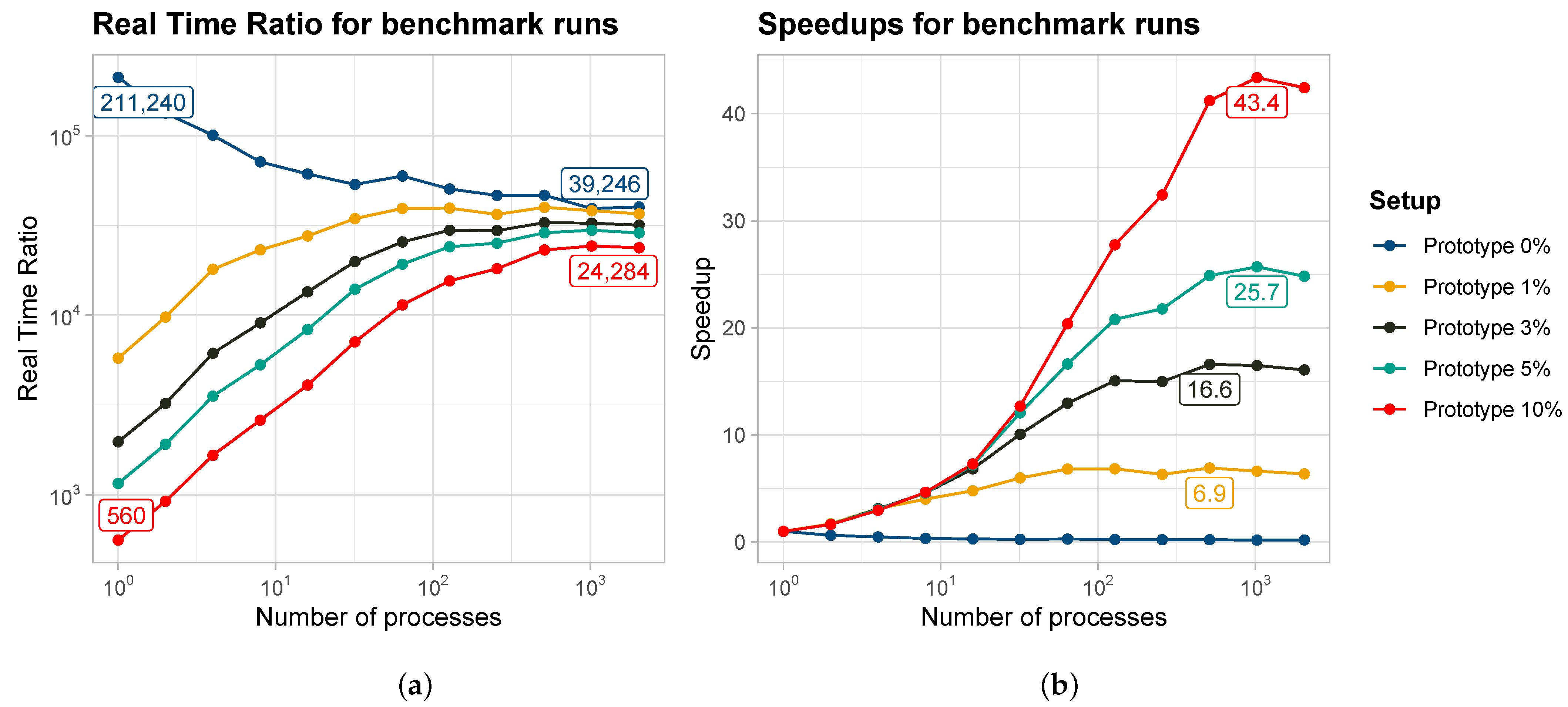
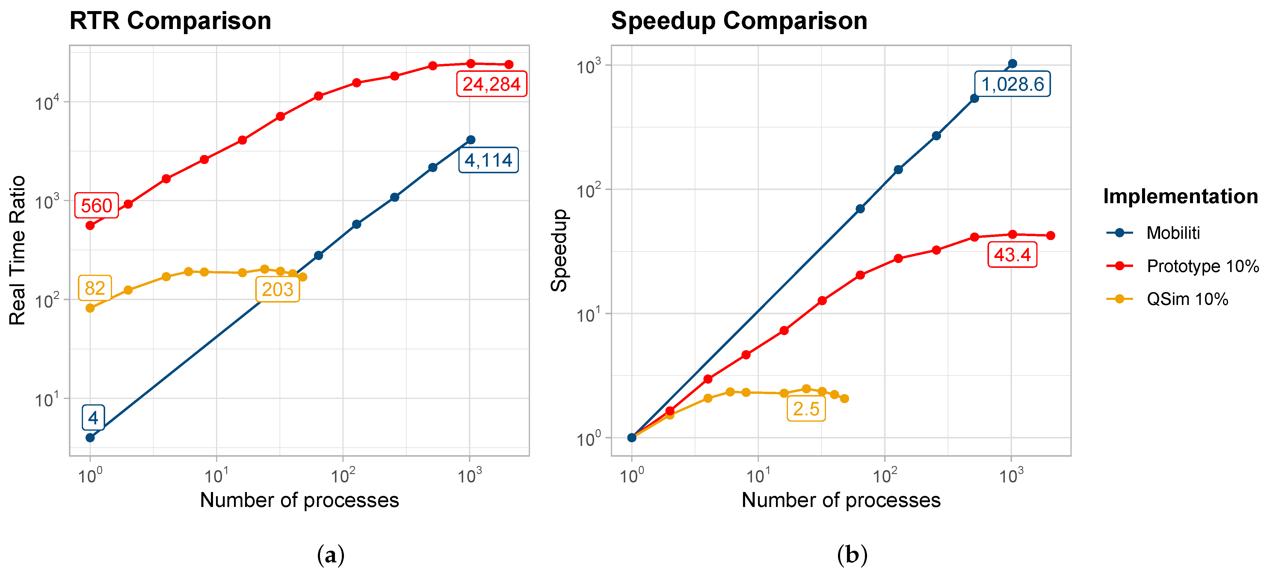
3.1. Overall Performance

Figure 5 presents the performance outcomes for different sample sizes of the Metropole Ruhr scenario using RTR (Real-Time Ratio) (Figure 5a) and speedup (Figure 5b) as indicators. The RTR indicates the ratio between simulated time and computation time. For example, an RTR of 100 indicates that it takes one second to calculate 100 simulated seconds. Compared to a more traditional measure such as overall runtime, the RTR is independent of the amount of simulated time and allows for a better estimate of the simulation performance.
Focusing on the largest setup displayed in red, which includes a 10% sample of the original population, we can see that an RTR of 560 is achieved when executed using a single process and a maximum RTR of 24,284 is reached for 1024 processes. These values correspond to a speedup of 43.4 as shown in Figure 5b.
As expected, the highest RTR of 211,240, is observed for the 0% setup on a single process, as shown in Figure 5a. This is because no inter-process communication slows down execution. As the number of processes increases, the RTR decreases but stabilizes around 40,000 for both 1024 and 2048 processes. Since this setup involves no actual simulation work and only handles communication between neighboring processes, the observed RTR values represent the baseline performance achievable with the current communication strategy of the application.
The 5%, 3%, and 1% setups in Figure 5a show proportionally higher RTR values compared to the 10% setup when executed on a single process. For example, the 1% setup is approximately 10 times faster than the 10% setup, achieving an RTR of 5765 on a single process. For larger process counts, the RTR for those setups ranges between those of the 10% and 0% setups. Notably, the 1% setup achieves nearly the same value as the 0% setup with 1024 processes, reaching an RTR of 38,182.
The key takeaway from these results is that, for large process counts, the difference in RTR across different setups becomes less significant. While the 1% setup achieves an RTR 10 times higher than the 10% setup on a single process, it is only 1.5 times faster when executed on 1024 processes. This suggests that, although there is some overhead in larger setups, it remains highly beneficial to run large simulations in a distributed manner. Examining the achieved speedups for the different setups shown in Figure 5b makes this more apparent. The 10% setup, which performs the most computational work, benefits the most from scaling across more processes, achieving a speedup of 43.4 with 1024 processes. In contrast, the 1% setup reaches a speedup of 6.8 with 64 processes, which is already close to its maximum speedup of 6.9 on 512 processes. The speedup values of 16.6 for the 3% setup and 25.7 for the 5% setup fall between those of the 10% and 1% setups, aligning well with the scaled sample sizes of their respective configurations. This suggests that, although there is some overhead in larger setups, it remains highly beneficial to run large simulations in a distributed manner. It can be expected that the RTR for even larger setups will remain within the same order of magnitude.

3.2. Latency as a Limiting Factor

To understand where time is spent during the simulation, we conduct an analysis of the individual algorithm steps. Figure 6 presents average durations to execute one simulation time step, where blue colors represent time spent calculating the traffic simulation as described in steps 1 to 4 in Section 2.3. Yellow colors depict execution times related to inter-process communication, covering steps 1 to 3 from Section 2.4.
In Figure 6a, which presents relative average shares of execution time by algorithm phase for the 10% setup, we observe that the time spent computing the traffic simulation decreases as more computing processes are utilized. The major share of computing time is spent on calculating the network dynamics of the simulation, specifically in the move nodes and move links steps. As the number of processes increases, the average time spent calculating the simulation approaches that of the 0% baseline run, as each process only calculates traffic for a very small share of the simulated traffic network. In contrast, the relative amount of time spent on communication—depicted in yellow shades—increases for a larger number of processes. The send and handle steps, which include serializing and deserializing messages, require only a minor share of computing time in the communication phase. The majority of time is spent in the receive step, which includes waiting for neighboring processes that may be slower in executing the traffic simulation, as well as the time required to transfer messages over the communication network. Figure 5 illustrates that in setups with a large number of processes, the time spent on communication largely determines the overall execution time, explaining the plateauing RTR observed in Figure 5a.
Figure 6b presents the absolute average durations of the various algorithm phases for the 0% setup, where no simulation work is performed. The results indicate that the operation time of the simulation framework remains consistently below one microsecond per time step, regardless of the number of processes. However, communication times exhibit significant variability. Similar to the relative values shown in Figure 6a, a substantial portion of the communication phase is dedicated to the receive phase of the algorithm. The time spent in the send and handle phases stabilize at approximately 3.5 µs and 1.5 µs.
Closer inspection of the absolute durations in Figure 6b reveals an increase in the duration of the receive phase as the number of processes grows. For example, with two processes, the average receive duration is 1.3 µs, while the maximum duration of 22 µs is observed with 512 processes. Since no simulation work is performed in the 0% setup, only empty messages are exchanged between processes to synchronize neighboring partitions at each simulation time step. Consequently, the observed timings for the 0% setup are primarily dictated by message-passing latency.
Table 1 presents the average and maximum number of neighbors for different process counts. From the table, we observe that as the number of processes increases, the average number of neighbors per partition approaches six, while the maximum number of neighbors stabilizes around 20. Additionally, the table shows the receive phase duration normalized by the average number of neighbors, which increases as the number of processes grows. In contrast, when normalized by the maximum number of neighbors, the receive phase duration remains constant at approximately 1 µs, regardless of the number of processes.
This observation suggests that the overall time spent in the receive phase is primarily driven by the maximum number of neighbors. This is intuitive, as a larger number of neighbors leads to more messages to process, thereby extending the communication time. Since all processes must wait for the process with the largest number of neighbors to complete its communication, the total communication time is dictated by this maximum. Interestingly, the receive duration normalized by the maximum number of neighbors shows constant values of 1 µs regardless of whether the configuration is executed on a single compute node (up to 16 processes) or on multiple computing nodes (32 processes and more).

3.3. Load Balancing as a Limiting Factor

As described in Section 2.4, the receive step of the communication phase encompasses both synchronization overhead between processes and the time required to transmit messages over the communication network. We will now examine the different timings of the coordination step to identify the limiting factors in various simulation setups, utilizing tracing data from individual time steps. In the following section, we are using the following wording to refer to the different phases of the coordination step:
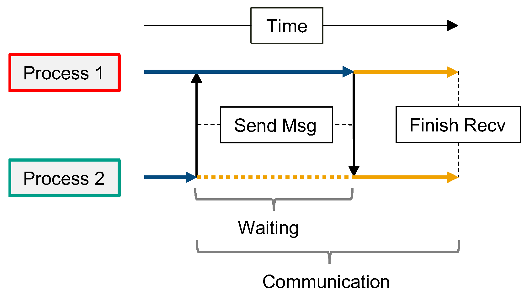
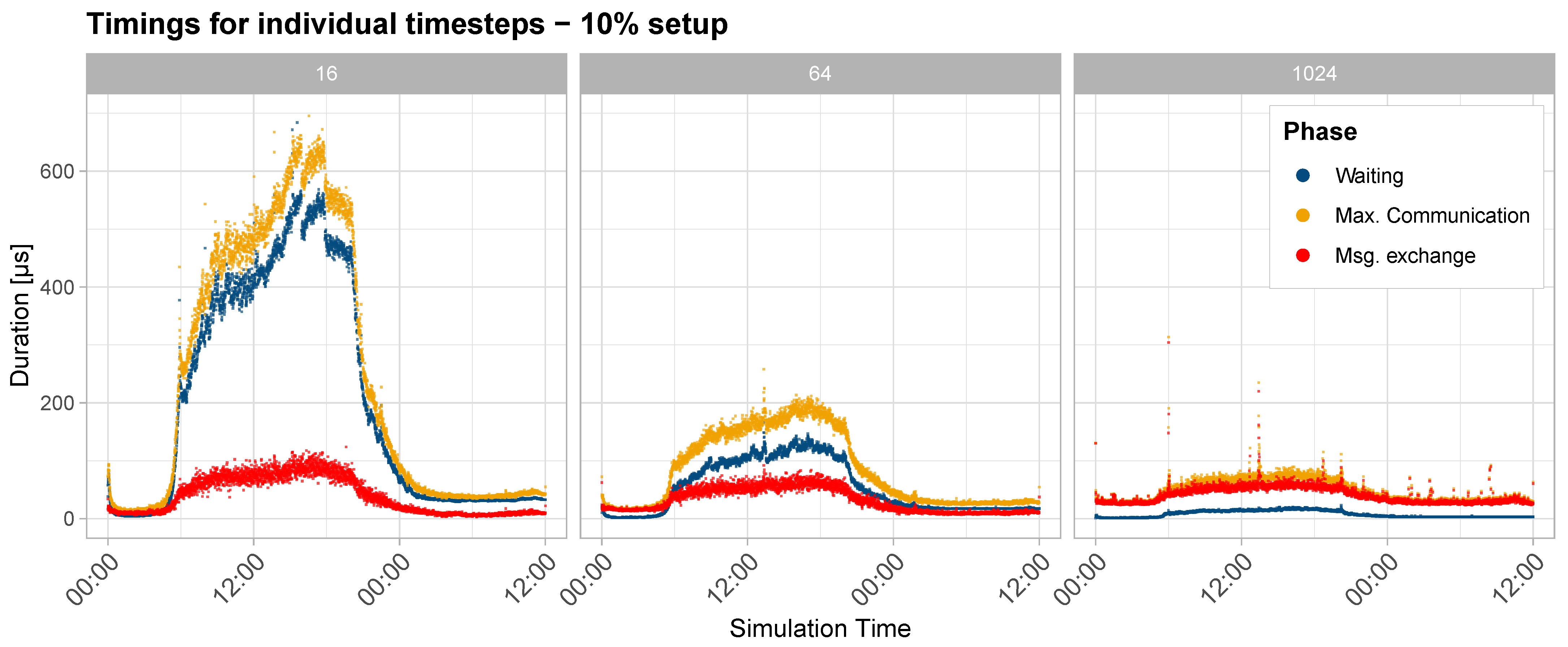
  • Wait time: To measure load imbalances, we use the difference between the fastest and slowest processes during a simulation time step. In Figure 3 the time spent computing a time step in the simulation is indicated by blue arrows. Figure 3 illustrates how faster processes must wait for slower processes to finish the simulation computation before adjacent processes can exchange messages. Large waiting times indicate unbalanced computational loads, while small waiting times suggest that each process handles a similar amount of work.
  • Maximum communication time: Also shown in Figure 3 is the maximum time any process spends in the communication phase. This includes the waiting time and the time to transmit messages over the communication hardware.
  • Message exchange time: The message exchange time cannot be measured directly in our application, as waiting for other process and transmitting messages occur in a single MPI Recv call. However, we can derive the time spent exchanging messages by subtracting the wait time of one simulation time step from the maximum communication time any process experienced. This duration corresponds to the straight yellow part of the arrows depicted in Figure 3.
Figure 7 displays timings for all three phases over the simulated day for configurations run with 16, 64, and 1024 processes of the 10% setup. The waiting times, represented in blue, show the differences between the fastest and slowest execution times for simulation computation. Maximum communication times are shown in yellow, and message exchange times are indicated in red. The timings are averaged over 30 simulated time steps to reduce the amount of tracing data written to disk.
An examination of the waiting times, as depicted in Figure 7, reveals that load imbalances closely follow the pattern of overall traffic volume throughout the simulated day. Starting around 5 a.m., waiting times increase in all configurations, peaking in the late afternoon, and then decrease steeply between 4 pm and midnight. In the 16 process configuration, waiting times range from 200 µs to 550 µs. Maximum communication times show a similar pattern, but are consistently higher than the wait times, with a peak of 650 µs observed in the early afternoon. The computed durations for message exchange also follow the overall traffic volume pattern but are significantly lower, ranging from 50 µs to 100 µs in the 16 process configuration.
In the 1024 process configuration, the situation is quite different. Load imbalances, as indicated by the wait times, are significantly smaller, with values as low as 10 µs per time step. Although the maximum communication times remain highest during periods of heavy traffic, the curve is less pronounced compared to configurations with fewer processes. The maximum communication times in the 1024 process configuration range from 50 µs to 80 µs. Since load imbalances in this configuration are minimal, the communication time is largely determined by the message exchange time, which is indicated in red.
The timings for the 64 process configuration exhibit characteristics of both the 16 and 1024 process configurations. Like the 16 process setup, load imbalances, indicated by waiting times, track the simulated traffic volumes over the day. However, the load imbalances are much smaller, ranging from 50 µs to 140 µs during busy periods. Maximum communication times are also smaller than in the 16 process configuration, with values between 100 µs and 200 µs. Timings for the message exchange are comparable to those observed in the 1024 process configuration and range between 50 µs and 80 µs during high traffic periods.
The data for the 16 process configuration indicates that communication overhead for smaller numbers of processes is primarily driven by computational load imbalances between processes. In contrast, the near equivalence of maximum communication and message exchange times in the 1024 process configuration suggests that the overhead in setups with many processes is primarily influenced by the time required to transmit messages over the communication hardware. Since each process in this configuration handles a relatively small portion of the simulation, the time spent waiting on other processes due to load imbalances is negligible compared to the time spent on inter-process communication.
Finally, an interesting observation arises when comparing the 16 and 1024 process configurations during periods of low traffic (at the start and end of the simulated day). In the 16 process configuration, the time spent on message exchange is much smaller during these periods compared to the 1024 process configuration. This suggests that for the 16 process configuration, which runs on a single compute node, the amount of data transferred is the primary factor driving message exchange times. Conversely, for the 1024 process configuration, which is distributed across 43 compute nodes, the lower variance in message exchange times indicates that the latency of the communication hardware is the dominant factor.

3.4. Performance Model

The performance of a distributed simulation depends on various parameters such as model size, communication hardware latency, and the number of neighbors per partition. Using insights from our previous work [9], we develop a performance model to predict runtime under changing conditions, incorporating slight adjustments based on the presented results.
The total runtime of a distributed computer program T ( p ) is determined by two major components: (1) the time required to solve the computational problem T c m p ( p ) , and (2) the time spent on communication T c o m m ( p ) . The total runtime T ( p ) depending on the number of processes p is calculated as:
T ( p ) = T c m p ( p ) + T c o m m ( p )
As demonstrated in Section 3.1, the computational time decreases as the number of processes increases. Assuming the computational load is evenly distributed, this relationship can be approximated by:
T c m p ( p ) = T c m p ( 1 ) p
Communication time depends on the latency t l per message and the number of neighbors N n ( p ) for each process. Following our previous work [9] we express T c o m m ( p ) as:
T c o m m ( p ) = N n ( p ) t l
Based on the Euler theorem for planar graphs, we previously assumed that N n ( p ) approaches six as p . However, as shown in Section 3.2, the maximum number of neighbors determines the time spent in communication. To account for this, we adjust our formula for N n ( p ) to:
N n ( p ) = 2 ( 10.5 p 1 ) ( p 1 ) / p
This equation converges to 21 for p , reflecting the maximum number of neighbors for the highest process count. The resulting performance model derives to:
T ( p ) = T c m p ( 1 ) p + t l · 2 ( 10.5 p 1 ) ( p 1 ) / p
Figure 8 illustrates the application of the performance model, comparing measured and predicted RTR values for the simulated case study (red line). While Table 1 suggests a latency of t l = 1 µ s per neighbor, the timings measured for the 10% sample indicate a higher average latency. This discrepancy arises because, in the 0% scenario, exchanged messages are minimal, consisting only of empty synchronization messages. In contrast, larger scenarios involve synchronization messages with larger payloads, leading to increased communication overhead. To account for this observation, the fitted model in Figure 8 assumes a latency of t l = 2 µ s .
We will now use the introduced performance model to analyze three scenarios, shown in Figure 8.
  • Large Scenario: For a simulation with 10 times more computational load (blue line), the computation on a single process is 10 times slower than the 10% scenario. However, a similar RTR can be achieved when increasing the number of processes 10-fold beyond the maximum number of processes used for the 10% scenario.
  • Future Communication Hardware: Assuming a future 10-fold improvement in communication hardware latency (yellow line), the application scales effectively across more processes. Faster hardware reduces the communication bottleneck, delaying the point where performance converges.
  • Ethernet Communication Hardware: Running the application on slower, standard Ethernet hardware (gray line) has a negative impact on performance. Assuming a latency of 10 µs per message exchange on a Gigabit Ethernet connection, the achievable RTR is significantly reduced. The model also predicts an earlier convergence in performance improvements, effectively limiting the scalability of the simulation.
  • Fewer Neighbors: If the maximum number of neighbors approaches the average assumed in our previous work (green line), the RTR improves significantly.
Overall, this confirms that the limiting factor for these types of simulations is the latency of the communication hardware, and (assuming a large enough computer) this results in a maximally reachable RTR that is independent of the scenario size. This also means that larger scenarios can be simulated at the same RTR as smaller scenarios, given a large enough computer. Other than Cetin et al. [9], we additionally find that the determining factor is the maximum number of neighbors, implying that there might be gains through a different domain decomposition algorithm. Evidently, communication hardware with lower latency will increase the maximally possible RTR.
This performance model enables predictions for hardware beyond HPC clusters, such as Ethernet-based systems. It helps evaluate whether transitioning to HPC hardware is beneficial and estimate computational requirements for simulations, aiding decisions on hardware investments or computing time applications.

4. Discussion

Building on the findings from the previous section, this section analyzes and contextualizes the results by highlighting strengths and potential limitations of the presented approach. Additionally, the presented results are compared against other work concerned about parallel and distributed traffic simulations.

4.1. Prototype Implementation

Previously, we have speculated that the runtime of the proposed message passing algorithm is bounded by the latencies in network communication. However, we were unable to measure this hypothesis for low latency networking hardware. With more computing power at hand, we can show that the execution times for a distributed queue simulation are in fact latency bound even on high-performance networking hardware like OmniPath 100. While the application scales well up to 1024 processes, we cannot show further speedups as the computational load for the utilized simulation scenario becomes insignificant compared to the communication overhead.
However, the introduced prototype also enables the computation of significantly larger models. Scaling the model size increases the computational load, which, in turn, reduces the relative impact of communication overhead. This suggests that the prototype is well-suited for handling larger simulation scenarios, where the balance between computation and communication shifts in favor of efficient scaling. Furthermore, our performance model supports this observation, predicting similar RTR for larger models, provided that a sufficiently large computing infrastructure is available.
As the number of processes increases, our results indicate that the impact of load imbalances becomes less significant. However, this scalability comes at the cost of reduced overall efficiency. As the computational load per process decreases, the time spent on messaging becomes dominant. This leads to processes spending a significant portion of their runtime idle, waiting for message exchanges to complete. As a result, the computational efficiency of the system declines with increasing process counts, reflecting the trade-off between scalability and efficiency.

4.2. Performance Model

The performance model developed in this work provides a useful framework for predicting the performance of distributed simulations under varying conditions, such as changes in model size or communication hardware. By incorporating both computational and communication components, the model helps estimate runtime and can guide decisions regarding resource allocation and hardware selection.
In this study, we refined the communication component of the model based on the finding that the maximum number of neighbors plays a significant role in determining communication time of the application. The updated model aligns well with measured performance, particularly in scenarios involving large numbers of processes.
However, the model has some limitations. One assumption is that the maximum number of neighbors converges to 21 as the number of processes increases. In practice, this may not hold true in all cases, particularly when using the METIS partitioning algorithm with default settings. METIS can produce partitions that are split into multiple parts, potentially resulting in significantly higher maximum neighbor counts than what we have observed. While the current model provides reasonable approximations, further refinement could improve its accuracy. Future work could explore the convergence of the maximum number of neighbors for large partition counts, as well as varying traffic network topologies.

4.3. Hardware Impacts

The performance model shows that the achievable RTR of the simulation highly depends on the computing hardware, especially the communication hardware. As demonstrated in the Future Communication Hardware scenario (Section 3.4), improvements in communication latency can significantly increase the achievable RTR. Conversely, running the application in a standard data center with slower communication hardware, such as regular Ethernet, leads to much lower RTR. This effect is illustrated in the Ethernet Communication Hardware scenario (Section 3.4).
In addition to supporting distributed computations across multiple nodes, the algorithm enables efficient parallel execution of the traffic simulation on a single multicore CPU. Compared to the previous shared memory implementation, the message-passing approach simplifies the implementation traffic simulation by explicitly handling inter-process communication via messages.
Advancements in CPU technology now focus on increasing the number of cores rather than clock speeds. For instance, the next-generation CPU at the NHR@ZIB HPC cluster provides 96 cores, compared to the 48 cores used in our experiments. This allows simulations with moderate partition counts to run on a single compute node, provided it has sufficient memory for the application’s data. Results from Section 3.2 for the 0% scenario show no difference in messaging latency between setups running on a single node and those distributed across multiple nodes. However, users without access to high-performance communication hardware will still benefit from processors with higher core counts. This is because the internal message exchange between processes on the same node is expected to be much faster than over Ethernet.

4.4. Possible Performance Improvements

Currently, our simulation scenarios do not fully utilize the capabilities of modern HPC clusters like NHR@ZIB, which provides over 100,000 computing cores. To fully take advantage of those capabilities, improvements on the application level as well as on the communication layer are possible.

4.4.1. Reducing Necessary Communication

The first option to improve the execution time of the presented prototype is changing the communication strategy on the application level. The goal of the proposed improvements is to reduce the communication that takes place during the simulation. Three primary strategies come to mind:
  • As indicated in by the analysis of the 0% setup, the communication time is primarily determined by the process with the largest number of neighbors. In our test runs involving large numbers of processes, the maximum number of neighboring domains reached up to 22, while the average remained around 6. By optimizing domain decomposition to reduce the maximum number of neighbors, we could decrease the number of exchanged messages, thereby reducing communication times. The objective of this optimization is to bring the maximum number of neighbors closer to the average value.
  • The current architecture requires synchronization of neighbor processes at every simulated time step. Turek [29] introduce a desynchronized traffic simulation, which shows linear scalability due to larger synchronization intervals. Instead of communicating instant updates of vehicles entering or leaving links, the synchronization interval in our approach could be increased by accounting for the time vehicles travel across links, as well as backwards travelling holes as suggested by Charypar et al. [30].
  • The synchronization between processes could be shifted from a conservative to an optimistic approach. In a simulation using an optimistic synchronization strategy, each process executes the traffic simulation independently, without explicitly waiting for synchronization messages. If a conflicting message is received from another process, the receiving process rolls back its simulation to the point where the message can be correctly applied. This approach reduces the need for synchronization messages at every time step. Chan et al. [19] present promising results using this approach, as discussed further in Section 4.5.

4.4.2. Improving Necessary Communication

The second option to improve the execution time of the presented prototype is changing the communication strategy at the level of the communication layer. Based on insights from Ghosh et al. [31] and Gropp et al. [32] (Chapters 2 and 3) the following strategies can be applied to speed up the necessary inter process communication:
  • Currently, our point-to-point communication involves three MPI-calls: ISend, MProbe, and MRecv, necessitating two network requests per message exchange. By adopting non-blocking counterparts for MProbe and MRecv, we could alleviate the constraints on the order of execution, though the total number of network requests would remain unchanged.
  • Transitioning to a higher level of abstraction for inter-process communication could also be beneficial. MPI v3 introduces collective communication primitives for distributed graph topologies. This could be particularly effective using the neighbor_alltoallv function.
  • Utilizing distributed graph topologies can optimize the physical locality of adjacent simulation domains, particularly for very large simulation setups. In many large HPC clusters, network topologies are arranged in a tree structure. This arrangement can result in neighbor partitions being placed on nodes located at opposite ends of the network tree. Consequently, messages must traverse multiple interconnects, leading to increased communication times. By leveraging MPI v3’s graph topology features, partitions can be mapped to computing nodes that are physically closer to each other. This placement reduces the number of interconnects that messages need to cross, thereby improving inter-process communication times and overall runtime efficiency.
  • MPI 3’s one-sided communication infrastructure allows asynchronous access to memory sections of remote processes through MPI windows, reducing the synchronization required for data exchange. However, this method requires careful management of memory offsets, making it more complex to implement.
Ghosh et al. [31] find that using neighbor collectives and one-sided communication can be 1.5 to 6 times faster compared to point-to-point communication. Combining architectural improvements with enhanced process synchronization could potentially reduce the computational time dedicated to inter process communication. This improvement enables both, higher achievable RTR, and better speedups when the application is scaled to more processes, particularly for smaller simulation setups.

4.5. Comparison with Other Work

We compare our findings with other work in the field, focusing on the current QSim implementation [6,9] within the MATSim ecosystem, the GPU-accelerated version by Strippgen [13], and the distributed traffic simulator Mobiliti [19], which targets HPC cluster environments.
Starting with the current Java-based QSim implementation, we use the simulation setup described in Section 3. Figure 9a illustrates RTR values for the current QSim implementation (orange) and our prototype (red). The Java-based QSim achieves an RTR of 82 on a single process, peaking at 202 with 24 processes. However, beyond six processes, the RTR plateaus at 191, resulting in a 2.5 times speedup compared to the single-process setup, as shown in Figure 9b. In contrast, our prototype achieves an RTR of 560 with a single process, a sevenfold improvement over QSim. This significant gain is likely due to Rust’s compact memory layout and better memory locality compared to Java’s reference-oriented approach. Compared to the QSim the presented prototype also scales much better with larger numbers of processes. The 10% setup simulated with the prototype reaches an RTR of 24,284 for 1024 processes, resulting in a 43.4 fold speedup compared to the single-process setup and a 119 times speedup relative to the current QSim implementation.
Strippgen [13] proposes a GPU-based implementation of the QSim, reporting execution times up to 70 times faster than the Java-based implementation. For a test scenario modeling the Zurich metropolitan region with a 50% sample size (comparable to our setup), their GPU implementation achieves an RTR of approximately 13,000. With modern hardware, even better performance could be expected. However, his work also shows that porting the QSim logic to a GPU programming model requires fundamental changes to MATSim’s data model to align with the SIMD (Single Instruction Multiple Data) paradigm used in hardware accelerators.
Chan et al. [19] evaluate the scalability of Mobiliti using a San Francisco Bay Area scenario with 3.7 million synthetic individuals. Their results show runtimes of 6 h for a single process, decreasing to 310 s with 64 processes and 21 s with 1024 processes. These correspond to RTRs of 4, 278, and 4114, respectively, with a maximum speedup of 1028 (Figure 9a,b). While Mobiliti demonstrates excellent scalability, the RTR shown in the experiment does not saturate, leaving its upper limits unclear. A smaller traffic model could have been used to determine the maximum achievable RTR of the Mobiliti traffic simulator. Alternatively, the same traffic model could have been tested on more processes to explore the limits of its scalability. Furthermore, the implementation of storage capacity constraints, important for spill-back effects, is mentioned as a future to do. Implementing these would require handling communication in the upstream direction of traffic, which could affect rollback rates and performance.
Finally, comparing single-core performance in Figure 9a, our prototype is 140 times faster than Mobiliti, despite their model being only 7.5 times larger. This suggests that our work optimizes an already efficient simulation algorithm, while the traffic flow implementation in Mobiliti appears to be more computationally expensive. Furthermore, an efficient software implementation offers benefits in terms of energy efficiency, a critical consideration in the context of global climate change [33].

5. Conclusions

We have successfully developed a prototype of a distributed mobsim, demonstrating the feasibility of extending the MATSim framework into a distributed traffic simulation. Our prototype outperforms the existing QSim implementation by a factor of 119, using a real-world scenario. With an RTR of 24,000, it is now possible to simulate an entire day in just 3.6 s.
Profiling indicates that with a sufficient number of processes, the computational time for traffic simulation becomes negligible, with the bulk of runtime spent on inter process communication. While this limits further speedups under the implemented communication strategy, it enables the execution of significantly larger simulation scenarios with similar RTRs. Nonetheless, we still see room for improvement by reducing the time spent on inter-process communication, by either optimizing the communication itself, or by reducing the amount of communication necessary.
The presented results indicate that the time for inter process communication depends on the maximum number of neighbors any process in the distributed simulation must communicate with. For the partitioning of the simulation domain, METIS [34] is used because it is generally available on HPC infrastructure. Future work on optimized communication times should include an evaluation of different partitioning algorithms on the performance of the simulation.
The results of the conducted benchmark indicate that optimizing the domain decomposition for minimal edge cuts or computational load on each partition is less critical compared to reducing the maximum number of neighbors for all partitions of a simulation setup, as the computation time is dominated by the number of message exchanges, which is related to the maximum number of neighbors.
Transitioning from a shared memory to a message-passing algorithm benefits simulation setups run on single machines as well. Unlike the current mobsim implementation, which achieves a 2.5 times speedup through parallelization, the prototype implementation scales well up to 16 processes, on a single machine, with a speedup of 7.3 compared to a simulation executed on a single core. This result suggests that adopting a message-passing approach to parallelize the MATSim traffic flow model would be beneficial, as future CPU generations will feature increasing numbers of processing cores.
The achieved speedups suggest that a distributed mobsim implementation should be integrated into the existing MATSim framework. To preserve the comprehensive functionality of the current framework without the need for extensive redevelopment, integration must be compatible with the JVM ecosystem and capable of leveraging high-performance networking hardware. Infinileap [35] and hadroNIO [36] are promising candidates for utilizing high-performance networking within the JVM.

Author Contributions

Conceptualization, J.L. and K.N.; Data curation, J.L.; Formal analysis, J.L. and P.H.; Funding acquisition, K.N.; Investigation, J.L. and P.H.; Methodology, J.L. and K.N.; Project administration, K.N.; Software, J.L. and P.H.; Supervision, K.N.; Validation, J.L. and P.H.; Visualization, J.L.; Writing—original draft, J.L.; Writing—review & editing, P.H. and K.N. All authors have read and agreed to the published version of the manuscript.

Funding

This research received no external funding.

Institutional Review Board Statement

Not applicable.

Informed Consent Statement

Not applicable.

Data Availability Statement

The source code of the presented protoype is available as GitHub repository (https://github.com/matsim-vsp/parallel_qsim_rust (accessed on 14 October 2024)). All benchmarks are run with the version captured in [10]. The input and output files can be found at https://doi.org/10.5281/zenodo.13928237 (accessed on 14 October 2024), a data repository hosted by CERN (European Organization for Nuclear Research) [11].

Acknowledgments

The authors gratefully acknowledge the computing time made available to them on the high-performance computer “Lise” at the NHR Center NHR@ZIB. This center is jointly supported by the Federal Ministry of Education and Research and the state governments participating in the NHR (www.nhr-verein.de/unsere-partner) (accessed on 14 October 2024). We acknowledge support by the Open Access Publication Fund of TU Berlin. This article is a revised and expanded version of a conference paper entitled High-Performance Simulations for Urban Planning: Implementing Parallel Distributed Multi-Agent Systems in MATSim, which was presented at the 23rd International Symposium on Parallel and Distributed Computing (ISPDC), Chur, Switzerland, 8–10 July 2024 [12]. The current work includes an expanded description of the methodology in general and the implemented algorithm in particular. Additionally, new simulation experiments using different sample sizes for our simulation setup are conducted, leading to a revised and more thorough results section. The discussion section is extended by including a comparison with other work in the field.

Conflicts of Interest

The authors declare no conflict of interest.

Abbreviations

CERNEuropean Organization for Nuclear Research
CPUCentral Processing Unit
FIFOFirst In First Out
GPUGraphics Processing Unit
HPCHigh-Performance Computing
JVMJava Virtual Machine
MATSimMulti-Agent Transport Simulation
mobsimmobility simulation
MPIMessage Passing Interface
ptpublic transit
RTRReal-Time Ratio
SIMDSingle Instruction Multiple Data

References

  1. Desa, U.N. World Urbanization Prospects 2018: Highlights; Technical report; United Nations: New York, NY, USA, 2018. [Google Scholar]
  2. Aleko, D.R.; Djahel, S. An efficient Adaptive Traffic Light Control System for urban road traffic congestion reduction in smart cities. Information 2020, 11, 119. [Google Scholar] [CrossRef]
  3. Xiong, C.; Zhu, Z.; He, X.; Chen, X.; Zhu, S.; Mahapatra, S.; Chang, G.L.; Zhang, L. Developing a 24-hour large-scale microscopic traffic simulation model for the before-and-after study of a new tolled freeway in the Washington, DC–Baltimore region. J. Transp. Eng. 2015, 141, 05015001. [Google Scholar] [CrossRef]
  4. Perumalla, K.; Bremer, M.; Brown, K.; Chan, C. Computer Science Research Needs for Parallel Discrete Event Simulation (PDES); Technical Report LLNL-TR-840193; U.S. Department of Energy: Germantown, MD, USA, 2022.
  5. Leiserson, C.E.; Thompson, N.C.; Emer, J.S.; Kuszmaul, B.C.; Lampson, B.W.; Sanchez, D.; Schardl, T.B. There’s plenty of room at the Top: What will drive computer performance after Moore’s law? Science 2020, 368, aam9744. [Google Scholar] [CrossRef] [PubMed]
  6. Horni, A.; Nagel, K.; Axhausen, K.W. The Multi-Agent Transport Simulation Matsim; Ubiquity Press: London, UK, 2016. [Google Scholar] [CrossRef]
  7. Dobler, C.; Axhausen, K.W. Design and Implementation of a Parallel Queue-Based Traffic Flow Simulation; IVT: Zürich, Switzerland, 2011. [Google Scholar] [CrossRef]
  8. Graur, D.; Bruno, R.; Bischoff, J.; Rieser, M.; Scherr, W.; Hoefler, T.; Alonso, G. Hermes: Enabling efficient large-scale simulation in MATSim. Procedia Comput. Sci. 2021, 184, 635–641. [Google Scholar] [CrossRef]
  9. Cetin, N.; Burri, A.; Nagel, K. A large-scale agent-based traffic microsimulation based on queue model. In Proceedings of the Swiss Transport Research Conference (STRC), Monte Verita, Switzerland, 19–21 March 2003. [Google Scholar]
  10. Laudan, J.; Heinrich, P. Parallel QSim Rust v0.2.0; Zenodo: Genève, Switzerland, 2024. [Google Scholar] [CrossRef]
  11. Laudan, J. Rust QSim Simulation Experiment; Zenodo: Genève, Switzerland, 2024. [Google Scholar] [CrossRef]
  12. Laudan, J.; Heinrich, P.; Nagel, K. High-performance simulations for urban planning: Implementing parallel distributed multi-agent systems in MATSim. In Proceedings of the 2024 23rd International Symposium on Parallel and Distributed Computing (ISPDC), Chur, Switzerland, 8–10 July 2024; pp. 1–8. [Google Scholar] [CrossRef]
  13. Strippgen, D. Investigating the Technical Possibilities of Real-Time Interaction with Simulations of Mobile Intelligent Particles. Ph.D. Thesis, Technische Universität Berlin, Berlin, Germany, 2009. [Google Scholar] [CrossRef]
  14. Wan, L.; Yin, G.; Wang, J.; Ben-Dor, G.; Ogulenko, A.; Huang, Z. PATRIC: A high performance parallel urban transport simulation framework based on traffic clustering. Simul. Model. Pract. Theory 2023, 126, 102775. [Google Scholar] [CrossRef]
  15. Gong, Z.; Tang, W.; Bennett, D.A.; Thill, J.C. Parallel agent-based simulation of individual-level spatial interactions within a multicore computing environment. Int. J. Geogr. Inf. Sci. 2013, 27, 1152–1170. [Google Scholar] [CrossRef]
  16. OpenMP Architecture Review Board. OpenMP Application Programming Interface; OpenMP Architecture Review Board: Atlanta, GA, USA, 2023. [Google Scholar]
  17. Qu, Y.; Zhou, X. Large-scale dynamic transportation network simulation: A space-time-event parallel computing approach. Transp. Res. Part C Emerg. Technol. 2017, 75, 1–16. [Google Scholar] [CrossRef]
  18. Bragard, Q.; Ventresque, A.; Murphy, L. Self-Balancing Decentralized Distributed Platform for Urban Traffic Simulation. IEEE Trans. Intell. Transp. Syst. 2017, 18, 1190–1197. [Google Scholar] [CrossRef]
  19. Chan, C.; Wang, B.; Bachan, J.; Macfarlane, J. Mobiliti: Scalable Transportation Simulation Using High-Performance Parallel Computing. In Proceedings of the 2018 21st International Conference on Intelligent Transportation Systems (ITSC), Maui, HI, USA, 4–7 November 2018; pp. 634–641. [Google Scholar] [CrossRef]
  20. Xiao, J.; Andelfinger, P.; Eckhoff, D.; Cai, W.; Knoll, A. A Survey on Agent-based Simulation Using Hardware Accelerators. ACM Comput. Surv. 2019, 51, 1–35. [Google Scholar] [CrossRef]
  21. Zhou, H.; Dorsman, J.L.; Snelder, M.; Romph, E.d.; Mandjes, M. GPU-based Parallel Computing for Activity-based Travel Demand Models. Procedia Comput. Sci. 2019, 151, 726–732. [Google Scholar] [CrossRef]
  22. Saprykin, A.; Chokani, N.; Abhari, R.S. GEMSim: A GPU-accelerated multi-modal mobility simulator for large-scale scenarios. Simul. Model. Pract. Theory 2019, 94, 199–214. [Google Scholar] [CrossRef]
  23. Saprykin, A.; Chokani, N.; Abhari, R.S. Accelerating agent-based demand-responsive transport simulations with GPUs. Future Gener. Comput. Syst. 2022, 131, 43–58. [Google Scholar] [CrossRef]
  24. Message Passing Interface Forum. MPI: A Message-Passing Interface Standard Version 4.1. November 2023. Available online: https://www.mpi-forum.org/docs/mpi-4.1/mpi41-report.pdf (accessed on 6 February 2024).
  25. Vega-Gisbert, O.; Roman, J.E.; Squyres, J.M. Design and implementation of Java bindings in Open MPI. Parallel Comput. 2016, 59, 1–20. [Google Scholar] [CrossRef]
  26. Gabriel, E.; Fagg, G.E.; Bosilca, G.; Angskun, T.; Dongarra, J.J.; Squyres, J.M.; Sahay, V.; Kambadur, P.; Barrett, B.; Lumsdaine, A.; et al. Open MPI: Goals, Concept, and Design of a Next Generation MPI Implementation. In Proceedings of the Recent Advances in Parallel Virtual Machine and Message Passing Interface, Budapest, Hungary, 19–22 September 2004; Springer: Berlin/Heidelberg, Germany, 2004; pp. 97–104. [Google Scholar] [CrossRef]
  27. Karypis, G.; Kumar, V. Multilevelk-way Partitioning Scheme for Irregular Graphs. J. Parallel Distrib. Comput. 1998, 48, 96–129. [Google Scholar] [CrossRef]
  28. Horni, A.; Nagel, K.; Axhausen, K. MATSim User Guide; Technische Universität Berlin: Berlin, Germany, 2024. [Google Scholar]
  29. Turek, W. Erlang-based desynchronized urban traffic simulation for high-performance computing systems. Future Gener. Comput. Syst. 2018, 79, 645–652. [Google Scholar] [CrossRef]
  30. Charypar, D.; Axhausen, K.W.; Nagel, K. Event-Driven Queue-Based Traffic Flow Microsimulation. Transp. Res. Rec. 2007, 2003, 35–40. [Google Scholar] [CrossRef]
  31. Ghosh, S.; Halappanavar, M.; Kalyanaraman, A.; Khan, A.; Gebremedhin, A.H. Exploring MPI Communication Models for Graph Applications Using Graph Matching as a Case Study. In Proceedings of the 2019 IEEE International Parallel and Distributed Processing Symposium (IPDPS), Rio de Janeiro, Brazil, 20–24 May 2019; pp. 761–770. [Google Scholar] [CrossRef]
  32. Gropp, W.; Hoefler, T.; Thakur, R.; Lusk, E. Using Advanced MPI: Modern Features of the Message-Passing Interface; MIT Press: Cambridge, MA, USA, 2014. [Google Scholar]
  33. Lastovetsky, A.; Manumachu, R.R. Energy-efficient parallel computing: Challenges to scaling. Information 2023, 14, 248. [Google Scholar] [CrossRef]
  34. Karypis, G.; Kumar, V. Multilevel Algorithms for Multi-Constraint Graph Partitioning. In Proceedings of the SC ’98: Proceedings of the 1998 ACM/IEEE Conference on Supercomputing, Orlando, FL, USA, 7–13 November 1998; p. 28. [Google Scholar] [CrossRef]
  35. Krakowski, F.; Ruhland, F.; Schöttner, M. Infinileap: Modern High-Performance Networking for Distributed Java Applications based on RDMA. In Proceedings of the 2021 IEEE 27th International Conference on Parallel and Distributed Systems (ICPADS), Beijing, China, 14–16 December 2021; pp. 652–659. [Google Scholar] [CrossRef]
  36. Ruhland, F.; Krakowski, F.; Schöttner, M. hadroNIO: Accelerating Java NIO via UCX. In Proceedings of the 2021 20th International Symposium on Parallel and Distributed Computing (ISPDC), Cluj-Napoca, Romania, 28–30 July 2021; pp. 25–32. [Google Scholar] [CrossRef]
Figure 1. Intersection in the simulated network. Vehicles queue at the end of a link and can cross an intersection once the simulation time has advanced to their earliest exit times. Additionally, the releasing link has to have sufficient flow capacity, and the receiving link sufficient storage capacity. Links crossing a computational domain boundary are divided into two parts: The downstream part manages the queue, storage-, and flow-capacities. The upstream part mirrors the storage capacity. Vehicles and capacity updates are exchanged as messages in between partitions.
Information 16 00116 g001
Figure 2. Example simulation network divided into four domains: Each network partition is managed by one computing process which receive an individual numerical rank by which they can be identified. Links crossing a domain boundary are managed by the downstream process and establish a neighbor relationship between the processes they connect. Processes only communicate with neighbor processes.
Information 16 00116 g002
Figure 3. Schema of the timings to coordinate two simulation processes for one time step: Process 1 requires more time to calculate its share of the simulation (blue arrow) than process 2. Process 2 sends its message and waits until process 1 finishes work and sends its message as well (yellow dotted arrow). Messages are transmitted over the communication hardware after both processes have called send (straight yellow arrow).
Information 16 00116 g003
Figure 4. The central section of the network used in the example runs. Links are colored by partition.
Information 16 00116 g004
Figure 5. (a) Real-Time Ratio of different benchmark runs. Real-Time Ratio is used because this measure is independent of the amount of simulated time, in contrast to the absolute execution time. (b) speedups for the same benchmark runs. The highest speedup value is achieved for the largest scenario.
Information 16 00116 g005
Figure 6. Timings for performing one time step in the simulation, distinguished by simulation work (blue shades) and message exchange (yellow shades). The timings are shown for setups with different number of processes. (a) Relative duration to perform one simulation time step for the 10% setup. (b) Absolute durations to perform one simulation time step for the 0% setup.
Information 16 00116 g006
Figure 7. Average timings measured for 30 simulation steps. Waiting times are shown in blue, maximum communication times in yellow and times to exchange messages in red. Timings are shown for different setups with 16, 64 and 1024 processes.
Information 16 00116 g007
Figure 8. Fit of a performance model for the Prototype 10% scenario in red. Predictions of possible RTR for using the fitted model: (1) Large Scenario in blue, (2) Fast Communication Hardware in yellow, reduced maximum number of neighbors in green.
Information 16 00116 g008
Figure 9. (a) RTR of different simulation implementations. RTR is used because this measure is independent of the amount of simulated time, in contrast to the absolute execution time. (b) speedups for the same simulation implementations.
Information 16 00116 g009
Table 1. Neighbor relationships produced by the partitioning algorithm. The average number of neighbors for larger number of partitions is around 6. However, the maximum number of neighbors for any process is over 20 for large numbers of processes. Also shown is the duration for the receive phase of the 0% setup divided by the average number of neighbors and the maximum number of neighbors.
ProcessesAverage Number of NeighborsMaximum Number of NeighborsDuration in µs by Average Number of NeighborsDuration in µs by Maximum Number of Neighbors
21.001.01.41.4
42.503.00.90.7
84.256.01.41.0
165.257.01.20.9
325.259.01.71.0
645.7812.02.11.0
1286.0619.03.00.9
2566.2919.03.21.0
5126.0722.03.71.0
10245.7721.03.71.0
Disclaimer/Publisher’s Note: The statements, opinions and data contained in all publications are solely those of the individual author(s) and contributor(s) and not of MDPI and/or the editor(s). MDPI and/or the editor(s) disclaim responsibility for any injury to people or property resulting from any ideas, methods, instructions or products referred to in the content.

