Article

Application of VGG16 Transfer Learning for Breast Cancer Detection

Department of Computer Science, New Mexico Tech, Socorro, NM 87801, USA
*
Author to whom correspondence should be addressed.
These authors contributed equally to this work.
Information 2025, 16(3), 227; https://doi.org/10.3390/info16030227
Submission received: 26 January 2025 / Revised: 9 March 2025 / Accepted: 10 March 2025 / Published: 14 March 2025
(This article belongs to the Special Issue Real-World Applications of Machine Learning Techniques)

Abstract

:
Breast cancer is among the primary causes of cancer-related deaths globally, highlighting the critical need for effective and early diagnostic methods. Traditional diagnostic approaches, while valuable, often face limitations in accuracy and accessibility. Recent advancements in deep learning, particularly transfer learning, provide promising solutions for enhancing diagnostic precision in breast cancer detection. Due to the limited capability of the BreakHis dataset, transfer learning was utilized to advance the training of our new model with the VGG16 neural network model, well trained on the rich ImageNet dataset. Moreover, the VGG16 architecture was carefully modified, including the fine-tuning of its layers, yielding our new model: M-VGG16. The new M-VGG16 model is designed to carry out the binary cancer/benign classification of breast samples effectively. The experimental results of our M-VGG16 model showed it achieved high validation accuracy (93.68%), precision (93.22%), recall (97.91%), and a high AUC (0.9838), outperforming other peer models in the same field. This study validates the VGG16 model’s suitability for breast cancer detection via transfer learning, providing an efficient, adaptable framework for improving diagnostic accuracy and potentially enhancing breast cancer detection. Key breast cancer detection challenges and potential M-VGG16 model refinements are also discussed.

Graphical Abstract

1. Introduction

Breast cancer is the most common and deadliest type of cancer globally, particularly among women. Among over 100 types of cancers, breast cancer stands out due to its high prevalence and rising incidence rates, posing a serious health risk. In the United States alone, breast cancer claims the lives of approximately forty thousand women annually, accounting for around twelve percent of all cancer-related deaths [1]. By 2020, over two million new cases of breast cancer had been diagnosed, leading to 685,000 deaths worldwide [2]. Projections by the International Agency for Research on Cancer (IARC) indicate that by 2040, the annual breast cancer cases may exceed three million, with nearly one million related deaths, signifying a concerning 50% rise [3]. A lack of early diagnosis is contributing significantly to this increase. Traditional diagnostic techniques, such as mammography and physical breast exams, though effective, can be time-consuming, costly, uncomfortable, and potentially yield false results, exacerbating patient distress and delaying treatment. This underscores the need for advanced breast cancer detection methods that improve diagnostic accuracy, reduce erroneous results, and offer a more comfortable screening experience.
Several diagnostic methods for breast cancer are currently used, with mammography being the most common. This approach uses X-ray technology to detect abnormal lumps in breast tissue [4]. Other diagnostic methods include ultrasound, which differentiates between solid masses and fluid-filled cysts using high-frequency sound waves, and Magnetic Resonance Imaging (MRI), a non-invasive technique that generates detailed breast images and is particularly beneficial for patients with dense breast tissue or a higher cancer risk. Biopsies, where a small tissue sample is taken for microscopic analysis, confirm malignancy. Thermal imaging also detects blood flow changes and inflammation associated with breast cancer. The choice of diagnostic method often depends on factors like age, family history, and individual health. However, mammography’s challenges in detecting cancer in women with dense breast tissue may lead to missed diagnoses due to false negatives and unnecessary biopsies due to false positives [5]. These limitations have sparked growing interest in the use of machine learning (ML) via neural network deep learning (DL) models to enhance breast cancer detection and screening accuracy. ML algorithms can automatically detect tumors, classify lesions, predict treatment outcomes, and assess the cancer risk. This leads to more accurate diagnoses and can improve the recovery chances and quality of life for patients. ML models have shown promise in classifying and diagnosing breast cancer by analyzing patterns in imaging and genomic data, although challenges like large dataset requirements and integrating diverse data sources remain [6]. Moreover, some ML models may have limited clinical applicability due to algorithmic complexity and biases in the training data, which can lead to inaccurate predictions. Legal considerations also arise in the process of obtaining training datasets for ML modeling deployment. Such considerations include data privacy, informed consent, and potential unintended legal consequences. Figure 1 provides a visual summary of the differences between traditional machine learning and methods that use pre-trained models.
Due to the aforementioned challenges in obtaining rich training datasets, this research aimed to leverage transfer learning (TL) [8,9,10] as part of ML methodologies. This study aimed to improve the precision and effectiveness of systems designed for breast cancer detection. Our approach to achieving this goal was through the utilization of fine-tuned pre-trained ML models from other related domains. Such an approach aims to streamline diagnostic processes, reduce computational expenses, and improve generalization on the limited medical datasets at hand. TL, as a subfield of ML, enables models to adapt knowledge gained from one domain to a related domain, proving advantageous in tasks with limited labeled ML training datasets. In various ML applications, TL is employed in areas such as computer vision, natural language processing, speech recognition, recommendation systems, and even autonomous vehicles and healthcare diagnostics [8,11,12]. This TL methodology plays a fundamental role in advancing artificial intelligence, allowing models to learn and improve over time while significantly reducing the training time and computational resources. In computer vision, TL enhances tasks like image classification, object detection, and image segmentation, while in natural language processing, it aids in sentiment analysis, question answering, and language translation. By minimizing the training time and computational load, TL improves the model accuracy and generalization, even in resource-constrained settings.
For this study, we selected VGG16 (Visual Geometry Group 16-layer network) as the base model due to its established success in medical imaging, particularly in breast cancer detection. Its structured architecture facilitates effective transfer learning (TL) adaptation for histopathological classification. Additionally, its hierarchical convolutional structure effectively extracts spatial features while maintaining a relatively lightweight design for clinical applications [13]. Prior research, including studies by Mehra et al. [13], has validated VGG16’s reliability for classifying histopathological images, further supporting its suitability for breast cancer detection. By leveraging TL and fine-tuning, we aimed to enhance VGG16’s performance while preserving its practical advantages.
The key contributions of this study are outlined as follows:
  • A modified version of VGG16 tailored for breast cancer detection using transfer learning.
  • The application of class weighting to address dataset imbalances and improve the sensitivity to malignant cases.
  • The implementation of cyclical learning rate (CLR) scheduling to enhance the training efficiency and generalization.
  • An evaluation of VGG16 against other deep learning architectures, including VGG19, InceptionV3, and AlexNet, to justify its suitability for breast cancer detection.
  • An extensive BreakHis dataset evaluation using the accuracy, recall, precision, and AUC to assess benign vs. malignant classification.
In summary, our key contribution is the development of an optimized M-VGG16 model incorporating CLR scheduling and regularization techniques, achieving a recall of 97.91% and a precision of 93.22%. This surpasses previous approaches, particularly in minimizing false negatives—a crucial factor in clinical breast cancer detection.
This paper is structured as follows. Section 2 reviews the relevant literature, identifying key advancements and gaps within current breast cancer detection research. Section 3 provides a comprehensive description of the datasets, detailing their structure, characteristics, and suitability for this study’s objectives. Section 3 also outlines the methodology employed, including architectural choices for the TL models, specific adaptations for breast cancer classification, data preprocessing steps, hyperparameter optimization, and model training. Section 4 presents and analyzes the results obtained from our model, assessing its performance using evaluation criteria including the accuracy, precision, recall, and the area under the ROC curve (AUC). Section 5 concludes by discussing the improvements achieved through our proposed approach and outlines potential future work to further enhance the model’s effectiveness and applicability in breast cancer detection.

2. Related Works

In recent years, TL has emerged as a powerful technique in medical image analysis, significantly aiding in the detection and diagnosis of diseases like breast cancer. Given the complexity and variation in medical imaging data, developing highly accurate models often demands extensive labeled datasets, which can be challenging to obtain. TL mitigates this issue by utilizing models trained on extensive datasets like ImageNet and adapting them to specialized fields with limited data. This approach has shown promise in various medical applications, particularly in breast cancer detection, where accurate and early diagnosis is critical for effective treatment.
Pan and Yang [8] provided a foundational study on TL techniques, covering its core concepts and early applications. This work laid the groundwork for subsequent medical diagnostics applications, demonstrating that TL could significantly improve the model accuracy and efficiency. Shin et al. [9] demonstrated TL’s use in medical imaging, enhancing anomaly detection in X-rays and CT images by fine-tuning ImageNet-trained models. Hence, the authors showed TL improving the detection accuracy while reducing the need for extensive training on difficult-to-obtain medical-specific data.
Ghafoorian et al. [14] further demonstrated the effectiveness of TL in MRI analysis by using Convoluted Neural Networks (CNNs) pre-trained on large brain MRI datasets to detect multiple sclerosis lesions, yielding greater diagnostic accuracy than traditional methods. This research illustrated how TL enables models to generalize better, improving their performance on unseen images and thereby enhancing diagnostic reliability.
Li et al. [15] applied deep learning methods to analyze scan data for Alzheimer’s disease detection, using pre-trained models to identify metabolic patterns indicative of the disease. Their study, published in the Journal of Alzheimer’s Disease, highlighted TL’s potential to improve diagnostic accuracy while providing deeper insights into disease biomarkers.
TL’s role in histopathological image analysis, particularly for cancer detection, has been impactful. Litjens et al. [16] demonstrated that fine-tuning general image recognition models improved the classification performance on prostate cancer histopathology slides. This study emphasized the utility of trained models in enhancing the classification of cancerous tissues with limited histopathological datasets.
Mehra et al. [13] applied TL to breast cancer histopathological images using pre-trained VGG16, VGG19, and ResNet50 models. This research revealed that fine-tuning VGG16, in particular, provided high classification accuracy on the BreakHis dataset, achieving up to 92.6% accuracy and an AUC of 95.65%. The findings demonstrated that TL could outperform fully trained networks, especially when working with limited data.
Recent studies have continued to validate VGG16’s effectiveness in breast cancer detection. For example, Rana et al. [17] tested seven pre-trained models, including VGG16, on the BreakHis dataset, achieving a Balanced Accuracy (BAC) score of 78.04%. Although Xception and ResNet50 had slightly higher scores, VGG16 demonstrated reliable performance, highlighting its generalization ability across unbalanced datasets. This consistency underscores VGG16’s suitability for cancer detection tasks where diagnostic accuracy and generalization are essential, particularly with limited data.
Hossain et al. [18] further investigated VGG16’s application in breast ultrasound imaging. By combining VGG16’s convolutional layers with a custom fully connected network, they achieved an accuracy of 91%. The study addressed challenges unique to ultrasound imaging, such as speckle noise and texture complexity, by incorporating Grad-CAM [19] for feature localization, supporting VGG16’s suitability for clinical applications in complex imaging modalities.
In a related study, Prusty et al. [20] utilized VGG16 on the MIAS mammogram dataset, implementing data preprocessing techniques like CLAHE and Smote for balancing and contrast enhancement. Their model attained a test accuracy of 87.99%, demonstrating the utility of pre-trained models in environments with limited data availability, such as early cancer detection in mammography.
Our research extends prior studies [13,17,18,20,21] by enhancing VGG16’s architecture to improve its effectiveness in breast cancer detection. In addition to fine-tuning, we incorporated optimizations to improve the model generalization and classification performance. The choice of VGG16 was motivated by several key advantages:
  • Model Adaptability and Transfer Learning: VGG16’s sequential architecture facilitates smooth transfer learning and fine-tuning for medical imaging applications. Its structured convolutional layers enhance adaptation to histopathological datasets, ensuring reliable classification performance [13,17,22].
  • Generalization with Limited Data: Leveraging TL, VGG16 achieves high accuracy even with smaller labeled datasets, addressing a key challenge in medical imaging [13,16].
  • Comparison with Alternative Architectures: While models such as ResNet [23], DenseNet [24], and InceptionV3 [25] achieve strong performance in medical imaging, they have more complex architectures and require substantial computational resources. Vision Transformers (ViTs) [26] and EfficientNet [27] offer promising results but demand extensive training data and are more prone to overfitting [26,27]. In contrast, VGG16, with its structured convolutional design, remains a widely used model for transfer learning and histopathological classification [22]. The architecture balances feature extraction and adaptability, making it a reliable choice for breast cancer detection [9,13].
  • Study-Specific Enhancements: To further improve generalization and prevent overfitting, we integrated CLR scheduling, batch normalization, dropout, and L2 regularization. These enhancements contribute to classification stability, making VGG16 a computationally feasible and effective choice for breast cancer detection [28,29,30,31].

3. Our Approach

In this study, we explored a transfer learning approach for breast cancer classification using the VGG16 model modified with additional custom layers, M-VGG16, to improve the classification performance on the Breast Cancer Histopathological Image Classification (BreakHis) dataset. Given the challenge of limited annotated medical images, TL enabled the adaptation of existing feature representations for effectively classifying histopathological images of benign and malignant tumors.

3.1. Dataset and Preprocessing

The BreakHis dataset [32] comprises 9,109 microscopic images of breast tumor tissues collected from 82 patients, captured at magnification levels of 40 ×, 100×, 200×, and 400×. This dataset includes 2480 benign and 5429 malignant samples, with each image sized at 700 × 460 pixels and presented in an RGB color format. Developed with the P&D Laboratory, Brazil, BreakHis categorizes tumors as benign or malignant, with benign types like adenosis and fibroadenoma and malignant types including ductal and lobular carcinoma facilitating robust classification in histopathology studies.
To enhance the generalizability of our model in breast cancer detection, we trained M-VGG16 using images from all four available magnification levels in the BreakHis dataset (40×, 100×, 200×, and 400×). Unlike models trained on a single magnification level, this approach ensured that M-VGG16 could learn relevant features across different image resolutions [33], mirroring real-world clinical scenarios where multiple magnification levels are employed for diagnosis.
The breakdown of the dataset by the magnification factors is shown below in Table 1.
Each image filename stores essential information about the image itself, including the biopsy method, tumor class, tumor type, patient identification, and magnification factor. For example, an image filename such as SOB_B_TA-14-4659-40-001.png denotes that it is from a benign tubular adenoma tumor, slide ID 14-4659, captured at 40× magnification, and it is the first image from that slide. Figure 2 shows a sample of the BreaKHis dataset, illustrating benign and malignant tumor histology images at different magnifications.
To prepare the dataset for training, we applied a series of preprocessing steps to ensure consistency in the input size, enhance generalization, and address the class imbalance, as shown next.
  • Image Resizing and Normalization: Each image was resized to (224 × 224) pixels to match the input dimensions required by the VGG16 model [22]. Pixel values were rescaled to the range [0, 1] and divided by 255, standardizing the data to help stabilize training [9].
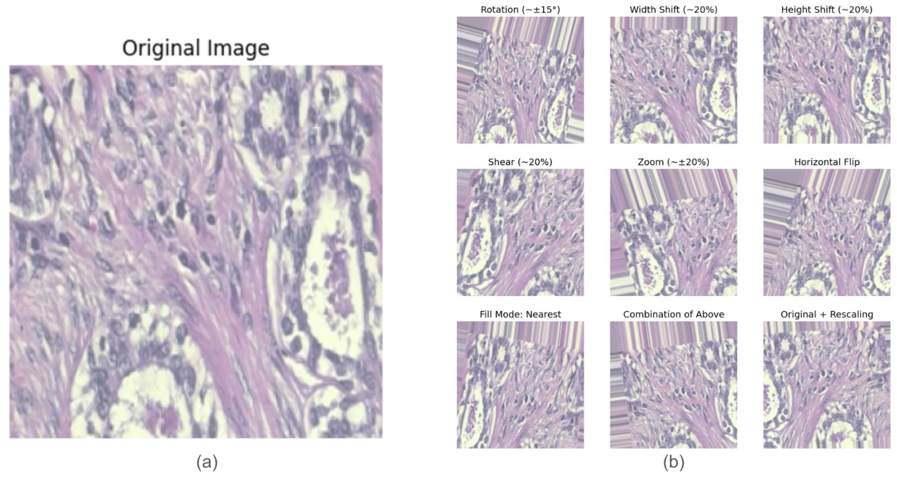
  • Data Augmentation: Data augmentation techniques were applied to improve the model generalization and reduce overfitting [21]. Figure 3 shows examples of images before and after augmentation. The augmentation transformations included the following:
    Rotation: Random rotations of up to 15 degrees.
    Translation: Horizontal and vertical shifts of up to 20%.
    Shearing: Up to 20% shearing transformation.
    Zooming: Random zooms of up to 20%.
    Horizontal Flipping: The creation of mirrored versions of the images.
  • Handling the Class Imbalance: Given the dataset’s imbalance, where malignant samples significantly outnumber benign ones, we calculated class weights to assign higher importance to the minority class (benign) during training and counter this disparity [34]. The class weights were computed using the following formula [35]:
    class weight = total samples number of classes × samples in class
    By computing the total number of samples and dividing this value by the combined product of the number of classes and the number of samples per class, this technique assigns higher weights to the minority class (benign). For instance, if benign samples are much fewer than malignant samples, this formula will assign a higher weight to the benign class. These weights increased the penalty for misclassifying benign samples, encouraging the model to learn patterns equitably across both classes [23]. By emphasizing the minority class in this way, class weighting reduced bias toward the majority class and enhanced the model’s ability to classify both benign and malignant cases accurately.
To optimize the training and validation balance, we evaluated several split ratios, 80/20%, 75/25%, and 70/30%, of the dataset samples for the training/validation%. We found out that a 70/30% split ratio yielded the best balance, ensuring a sufficiently large validation set to evaluate the model performance effectively while maintaining ample data for training. This setup was thus adopted for all ML experiments in this study. Additionally, we employed both stratified and random splitting strategies to assess the model robustness. The stratified split preserved the distribution of benign and malignant cases across the training and validation sets, mitigating class imbalance issues [36]. In contrast, a random split was also tested to evaluate the model’s performance under standard data partitioning. A comparative analysis of these methods is presented in Section 4.
These preprocessing steps were essential to prepare the dataset to be input into the M-VGG16-based TL model, optimizing it for feature extraction and enhancing the classification performance in breast cancer histopathology.

3.2. Model Architecture

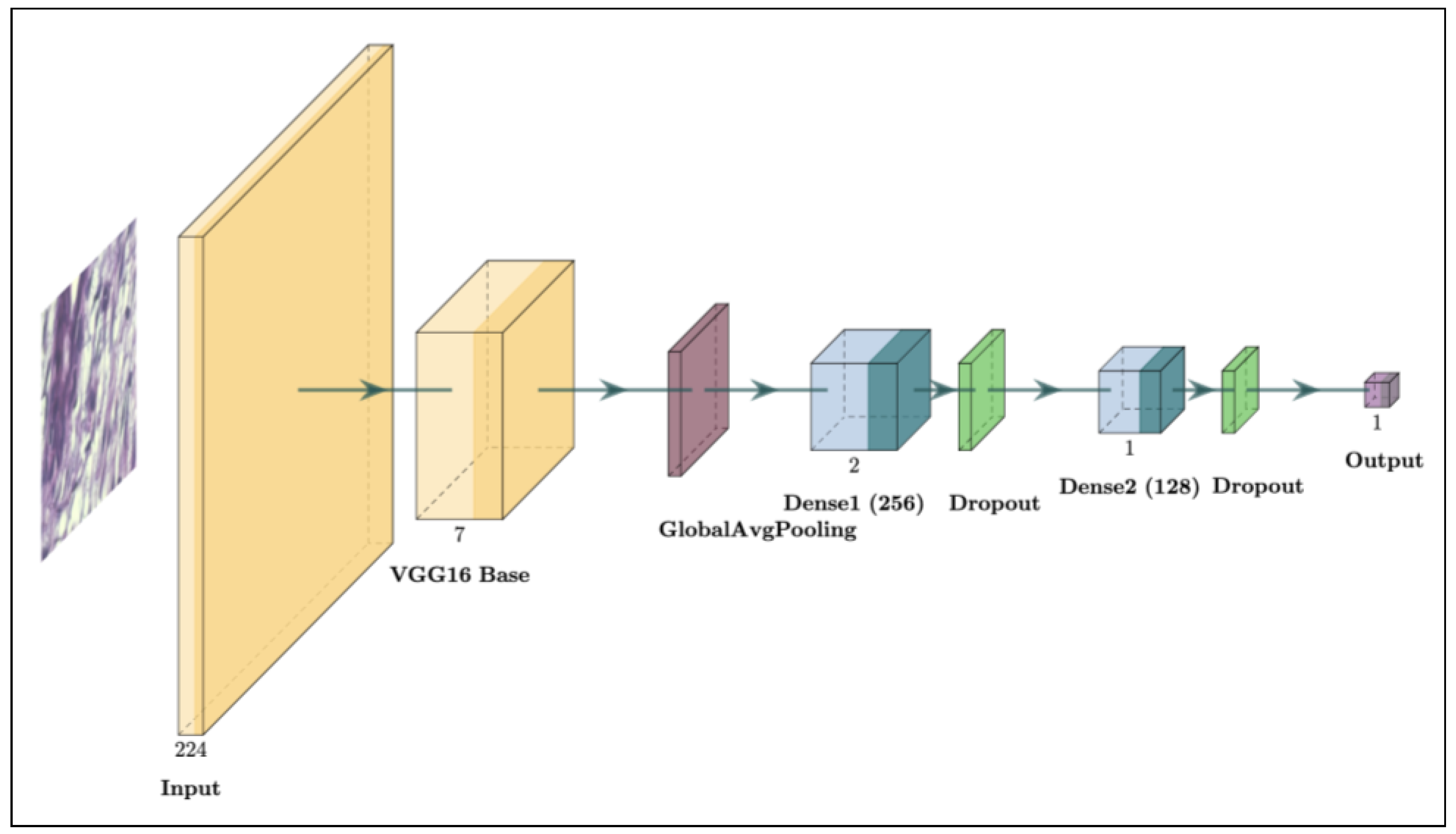
3.2.1. Base Model: VGG16

In this study, we employed the VGG16 [37] model as our base architecture due to its proven effectiveness in image classification and ability to extract hierarchical features efficiently. Developed by Simonyan and Zisserman in Oxford’s Visual Geometry Group (VGG), VGG16 is a deep convolutional neural network (CNN) pre-trained on the large-scale ImageNet dataset, which comprises over a million images across 1000 categories. This model includes 13 convolutional layers with uniform 3 × 3 filters, interspersed with max-pooling layers that reduce the spatial dimensions while retaining critical features, followed by three fully connected layers.
To make use of this pre-trained knowledge, we adapted VGG16 to classify histopathological images of benign and malignant tumors in the BreakHis dataset. By fine-tuning the last 12 layers of the model, we allowed it to adjust its learned features to the unique characteristics of breast cancer images, facilitating effective feature extraction without extensive dataset-specific training. This approach, known as transfer learning (TL), leverages VGG16’s robust, pre-trained feature extraction layers to achieve high classification accuracy while maintaining computational efficiency. This makes VGG16 especially suitable for medical imaging tasks, where models like ResNet or InceptionV3 may be prone to overfitting when applied to smaller datasets.
To adapt VGG16 to the requirements of binary classification, we modified the model by removing its original fully connected top layers. In their place, additional custom layers were added to capture domain-specific patterns in breast cancer histopathology images, as illustrated in Figure 4. This figure shows M-VGG16, which includes a sequence of layers specifically designed for binary classification. These architectural modifications, detailed in the figure, allow the model to capture essential patterns in histopathological images for more accurate differentiation between benign and malignant tumors. The architectural changes were as follows:
  • Global Average Pooling: A specialized layer, called GlobalAveragePooling2D, was introduced after the convolutional layers to replace the traditional Flatten layer. This pooling technique reduces the spatial dimensions of the feature maps, creating a more compact and generalized feature vector while reducing the risk of overfitting [38]. The Global Average Pooling layer computes the average output of each feature map, condensing it into a single value per map. This approach is effective in image classification tasks as it encourages the model to capture the global context rather than focusing on specific spatial locations, which can be advantageous in tasks like histopathological analysis where spatial features vary widely across samples.
  • Dense Layers: Two Dense layers with 256 and 128 units, respectively, were added after the pooling layer. Each dense layer uses the ReLU (Rectified Linear Unit) activation function to introduce non-linearity and enable the model to learn complex patterns within the data [39]. Dense layers are essential in transforming the compacted features into higher-level representations for binary classification. L2 regularization, with a penalty coefficient of 10 5 , was applied to both dense layers to help prevent overfitting by penalizing large weight values [31]. This regularization technique improved the model’s generalization by preventing overly complex fits to the training data, a key factor in medical imaging tasks where training datasets are often limited.
  • Batch Normalization and Dropout: Batch normalization layers were incorporated after each dense layer to standardize the outputs, stabilizing and accelerating the training process [29]. Batch normalization mitigates internal covariate shifts by normalizing the layer inputs, leading to faster convergence and reduced sensitivity to the initialization parameters. Following each batch normalization layer, a Dropout layer with a rate of 0.25 was added. To mitigate overfitting, dropout randomly deactivates parts of the network during each training phase, supporting more generalized learning outcomes [30]. This combination of normalization and dropout has been shown to improve both a model’s stability and robustness, especially in TL scenarios where overfitting can be common due to limited data.
  • Output Layer: A final fully connected layer with one output neuron and a sigmoid activation function was added to generate a probability score for binary classification. The sigmoid function outputs a value between 0 and 1, which can be interpreted as the probability of a sample belonging to the positive class [40]. If the probability is below 0.5, it indicates a higher likelihood of the tumor being benign; if the probability is 0.5 or higher, it indicates a higher likelihood of malignancy. This simple yet effective design makes it well suited for binary classification, ensuring clinically meaningful predictions [16,18].

3.2.2. Fine-Tuning the Base Model

To enable the model to learn domain-specific features more effectively, we fine-tuned the VGG16 base model by unfreezing the last 12 layers. This allowed the pre-trained layers to adjust their weights based on the new dataset while retaining the general features learned from the ImageNet dataset. Fine-tuning these layers helped the model capture subtle distinctions between benign and malignant histopathological images.

3.2.3. Compilation and Hyperparameters

The model was compiled using the Adam optimizer [41] and binary cross-entropy loss [42]. Gradient clipping [43] was applied to prevent exploding gradients, ensuring stable updates during training. The model was trained for a maximum of 50 epochs, with early stopping [44] to halt training if the validation loss did not improve for 5 consecutive epochs, preventing overfitting. The following key parameters were used: batch size = 32, initial learning rate = 10 4 , CLR cycle length = 10 epochs with base and max learning rates of 10 5 and 10 4 , respectively, L2 regularization coefficient = 10 5 , dropout rate = 0.25, early stopping patience = 5 epochs, and gradient clipping threshold = 1.0.
A cyclical learning rate (CLR) scheduler [28] was implemented (Figure 5), dynamically adjusting the learning rate between predefined minimum and maximum values. This strategy improved convergence by allowing the model to escape sharp local minima, promoting stability and generalization [28].
A custom callback was incorporated to monitor false positives and false negatives, providing additional performance insights beyond conventional accuracy metrics [45].

3.3. Comparative Analysis with Other Pre-Trained Models

To validate and compare the robustness of TL models, we applied the same architecture and parameter settings to other models such as InceptionV3 [46], AlexNet [47], and VGG19 [22]. These models were fine-tuned and adapted for the binary classification task of breast cancer detection in a manner consistent with the approach used for VGG16. To ensure a fair comparison, training parameters such as the optimizer, learning rate, batch size, and early stopping criteria were kept consistent across all models. This comparative analysis allowed us to assess the effectiveness and efficiency of VGG16 against other popular architectures, ultimately providing insights into the best model for histopathological breast cancer classification.

4. Result Analysis

To evaluate the effectiveness of our simulated model and also peer model simulations, we measured the accuracy, precision, recall, F1-score, and AUC for both the training and validation subsets. These metrics provided a comprehensive view of each model’s performance, enabling us to identify the most suitable model for our dataset. The metrics were calculated based on the counts of false positives (FPs), false negatives (FNs), True Positives (TPs), and True Negatives (TNs), allowing us to accurately assess each model’s predictive capabilities. Additionally, we tested several alternative base models with our customized layer configuration to ensure a fair comparison. Our results were then benchmarked against previous studies to contextualize the M-VGG16 model’s performance within the field. The following sections provide a detailed discussion of these evaluation metrics, the tabulated performance results, and visual representations of the outcomes.

4.1. Evaluation Metrics

We evaluated the effectiveness of our VGG16-based model using key performance indicators, including the accuracy, precision, recall, F1-score, and AUC. Each of these metrics provided valuable insights into the model’s ability to classify benign and malignant cases effectively, especially in the context of a binary classification problem with potential class imbalances. These metrics were calculated based on the counts of True Positives (TPs), false positives (FPs), True Negatives (TNs), and false negatives (FNs) obtained from the model’s predictions.
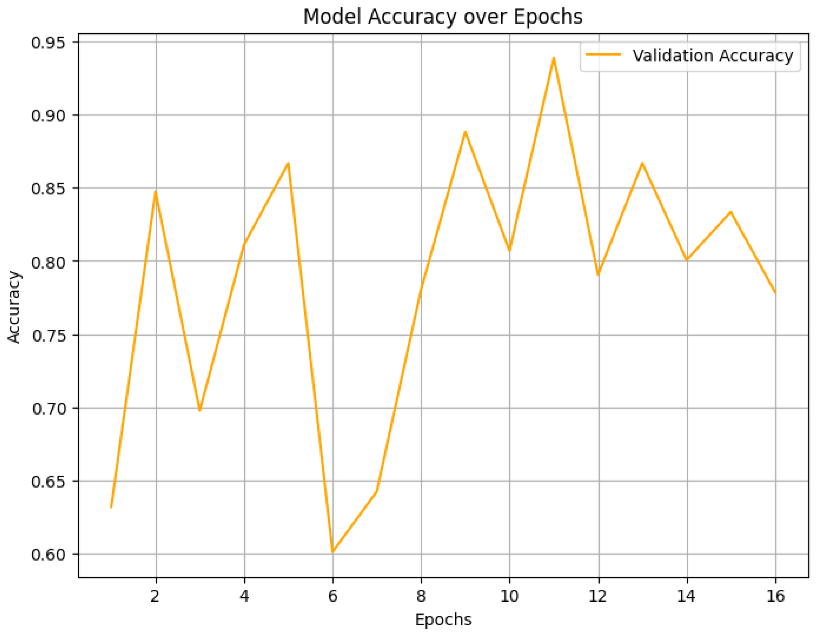
  • Accuracy: The proportion of the total correct predictions, calculated as
    Accuracy = T P + T N T P + F P + F N + T N .
    The accuracy provides a general measure of the model’s performance across both classes.
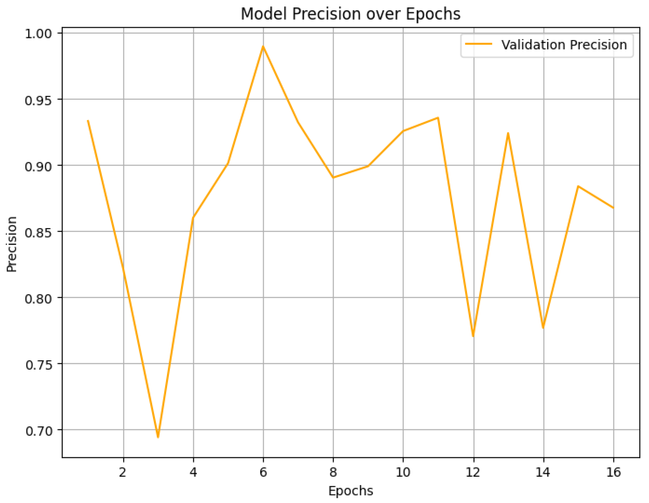
  • Precision: The ratio of correctly predicted positive samples to the total predicted positive samples, given by
    Precision = T P T P + F P .
    The precision evaluates the model’s accuracy in predicting malignant cases, which is crucial to minimize false alarms.
  • Recall: The ratio of correctly identified positive samples to all actual positive samples, defined as
    Recall = T P T P + F N .
    The recall is especially important in identifying malignant cases accurately to avoid missed detections.
  • F1-Score: A harmonic mean of the precision and recall, calculated as
    F 1 - Score = 2 × Precision × Recall Precision + Recall .
    The F1-score balances precision and recall, making it effective in handling class imbalances.
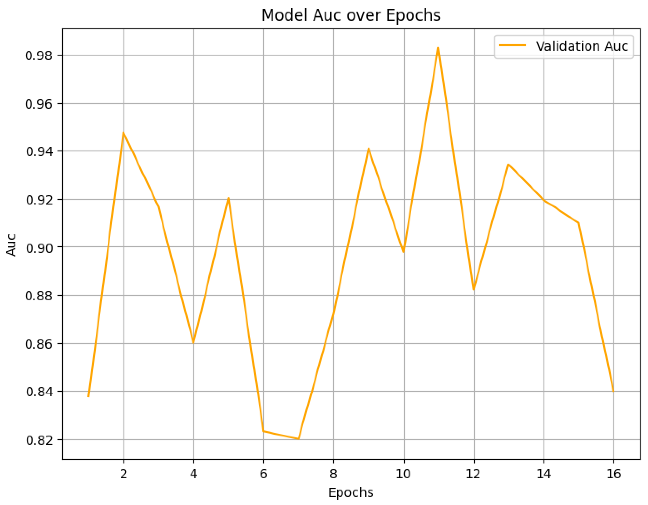
  • Area Under the ROC Curve (AUC): The AUC evaluates the model’s proficiency in distinguishing between classes by calculating the area beneath the Receiver Operating Characteristic (ROC) curve, which illustrates the relationship between the True Positive Rate (TPR) and the False Positive Rate (FPR). A higher AUC value signifies improved classification performance, showcasing the model’s ability to accurately distinguish positive instances and reduce the number of false positives. This metric provides a comprehensive evaluation of the model’s classification capabilities, which is essential for achieving accurate and reliable diagnostic results.
These metrics provided a thorough assessment of our model’s performance on both the training and validation datasets. Additionally, by applying these metrics across alternative base models with our customized layer architecture, we identified the best-performing model for this task. The following sections delve into the tabulated results and visual representations of these metrics, along with comparisons to results from previous studies to contextualize the effectiveness of our approach.

4.2. Final Performance Metrics

The model’s performance was evaluated across multiple epochs, revealing steady improvements in key metrics—the accuracy, precision, recall, AUC, and loss. Figure 6, Figure 7, Figure 8, Figure 9 and Figure 10 display the progression of these metrics on the validation dataset, with optimal performance observed at epoch 11 with a random split, preserved through early stopping and callback mechanisms.
Figure 6 shows the validation accuracy, peaking at 93.89% during the 11th epoch and declining afterward. Callback functions, including early stopping, preserved the model’s state at its peak performance, preventing overfitting and supporting generalization.
Figure 7 illustrates the precision trends, beginning at 0.9334, dipping to 0.6942 by the third epoch, and reaching an optimal balance at 0.9899 by the sixth epoch. Fine-tuning and adaptive learning rates contributed to the balanced precision by the end of training.
Figure 8 shows the recall progression, beginning at 0.4994 and reaching a peak of 1.0000 by the third epoch. Fluctuations, including a drop to 0.4232, were mitigated by early stopping and callbacks to maintain stability, critical for minimizing false negatives.
Figure 9 presents the AUC values, starting at 0.8378, rising to 0.9476 in the second epoch, and peaking at 0.9828 at epoch 11, reflecting the model’s improved discriminative capability.
Figure 10 shows the trend of the validation loss, starting at 0.6338, dropping to 0.3583 by the second epoch, and reaching a low of 0.1596 at epoch 11. Early stopping was applied to preserve this optimal performance by halting further training.
By epoch 16, early stopping was triggered as further improvements in the validation loss were negligible. This mechanism, along with other callback functions such as learning rate scheduling and custom metric tracking, preserved the model’s optimal state from epoch 11, where an ideal balance across key metrics, e.g., the validation accuracy, precision, recall, and AUC, was achieved. These callbacks played a critical role by dynamically adjusting the training parameters, preventing overfitting, and optimizing generalization.
Table 2 summarizes the final performance metrics obtained at this optimal epoch for the results both before and after augmentation using random and stratified data splits. The results indicate a significant improvement after augmentation, with the random split achieving higher accuracy (93.68%) and a higher AUC (0.9838), whereas the stratified split yielded superior recall (98.22%), ensuring fewer false negatives, which is an essential factor in breast cancer detection. Before augmentation, the model exhibited lower performance, with accuracy at 83.09%, recall at 93.80%, and an AUC at 0.9065, highlighting the necessity of augmentation in improving generalization and classification stability.
These final metrics reaffirm the model’s robustness and its suitability for diagnostic applications, demonstrating high classification performance across both partitioning strategies as shown in Table 2. The recall improvements observed in the stratified split reinforce its effectiveness in minimizing false negatives, which is particularly valuable in real-world clinical settings [48] where early cancer detection is critical.

4.3. Different Pre-Trained Models’ Performance Comparison

Table 3 summarizes the performance of each base model with our custom layering and cyclical learning rate (CLR) scheduler. While M-VGG16 and M-VGG19 achieved comparable accuracy (93.68% and 92.3%, respectively), M-VGG16 demonstrated a slightly higher recall (97.91%) compared to M-VGG19 (96.55%).
Table 4 presents a detailed comparison of the memory usage, inference time, and FLOPs across the models.
Beyond the classification performance, computational efficiency is crucial for real-time AI-based diagnostics. While M-VGG19 had comparable accuracy, its longer inference time (44.00 ms vs. 41.56 ms) and higher memory consumption (77.02 MB vs. 56.76 MB) make M-VGG16 a more efficient choice. M-InceptionV3, despite its lower computational cost (31.44 GFLOPs), had a higher inference time (58.20 ms) and greater memory usage (85.30 MB), making it less optimal for rapid diagnosis. M-AlexNet, though having the lowest GFLOPs (21.84) and fastest inference time (25.78 ms), compromised on accuracy (85.68%) and recall (83.95%), limiting its clinical applicability. M-VGG16 balanced the classification performance and computational cost, achieving a moderate GFLOPs requirement (1476.04), faster inference time (41.56 ms), and reduced memory footprint (56.76 MB), outperforming M-VGG19 and InceptionV3 in terms of resource efficiency. With high recall (97.91%) and precision (93.22%), M-VGG16 remains a computationally viable and effective candidate for real-time clinical breast cancer diagnostics.
To illustrate the performance of all the simulated models, Figure 11 presents a bar chart comparing the accuracy, precision, recall, and training time. M-VGG16 and M-VGG19 achieved the highest accuracy and recall, while M-AlexNet demonstrated the shortest training time.
The chart highlights trade-offs between the accuracy, recall, and training time across the models. Although M-AlexNet trained the fastest, it lagged in accuracy and recall compared to M-VGG16 and M-VGG19. M-VGG16 outperformed the other models in accuracy, precision, and recall due to its deeper architecture, consistent convolutional layers, and effective transfer learning approach. Fine-tuning the last 12 layers of the pre-trained VGG16 model enabled it to better adapt to the BreakHis dataset, leading to the improved classification of benign and malignant tumors. Additionally, applying regularization methods like dropout and L2 regularization mitigated overfitting, thereby ensuring the model maintained strong performance on the validation data.

4.4. Comparative Analysis with Previous Studies

The performance of the proposed M-VGG16 in this study was compared with other significant works that utilized VGG16-based architectures for breast cancer detection using the BreakHis dataset, and the comparison is summarized in Table 5. Our comparison was based on performance metrics reported in the published literature that specifically evaluated VGG16 models on the same dataset. While these studies provide benchmark results for standard and modified VGG16 versions, differences in the dataset splits, augmentation techniques, and hyperparameter configurations may introduce variability. Thus, variations in the experimental setups should be considered when interpreting the results.
While our M-VGG16 model demonstrated improved performance metrics compared to previous approaches, we note that variations in the experimental setups across studies may affect direct comparisons. The improvements in recall (97.91%) are particularly significant for clinical applications as they directly impact the reduction of false negatives. Future work would benefit from standardized evaluation protocols and statistical significance testing to further validate these performance gains.
The proposed M-VGG16 model exhibited strong recall (97.91%) and precision (93.22%), differentiating it from the standard VGG16 and other variants. While Agarwal et al. [49] achieved a higher accuracy (94.67%) using SMOTE preprocessing, their model’s recall was significantly lower (80.52%), increasing the very dangerous risk of misclassifying malignant cases as benign. Similarly, Singh et al. [50] reported a recall of 91.00%, which is competitive, yet still lower than the crucial recall performance metric achieved by our model. We can assert that our M-VGG16 model’s higher recall reduces false negatives, making it more effective for early cancer detection, where sensitivity is a key diagnostic priority.
Additionally, the M-VGG16 combination of CLR scheduling and fine-tuning enhances stability and generalization, ensuring consistent performance while maintaining computational feasibility for practical, computation-demanding applications [22,28,29,30]. These optimizations contribute to M-VGG16’s robustness in histopathological image classification, making it a practical and reliable candidate for breast cancer detection in clinical workflows.

4.5. Discussion

The effectiveness of our M-VGG16 model extends beyond accuracy and recall, making it a strong candidate for real-world deployment in breast cancer diagnostics. One of the key advantages of the model is its ability to minimize false negatives while maintaining computational efficiency, which is crucial in medical applications where timely and accurate predictions directly impact patient well-being. Our M-VGG16 achieves a comparable accuracy (93.68%) to deeper models like M-VGG19 (92.3%) while demonstrating a significantly higher recall (97.91% vs. 96.55%). This ensures fewer misclassified malignant cases, reducing the risk of delayed cancer diagnoses and improving early detection, which saves precious human lives.
A recall of 97.91% for M-VGG16, compared to 80.52% in Agarwal et al. [49] and 91.00% in Singh et al. [50], highlights the effectiveness of our model in minimizing false negatives. Although Agarwal et al. achieved slightly higher accuracy (94.67% vs. 93.68%), their lower recall indicates that a substantial number of malignant cases were misclassified as benign, which could lead to delayed intervention and a possible loss of human life. In contrast, M-VGG16 prioritizes sensitivity while maintaining strong precision (93.22%), ensuring that more malignant cases are correctly detected, reducing the risk of undiagnosed cancer progression, and ultimately enhancing early treatment strategies.
Beyond the model architecture, data augmentation played a crucial role in improving generalization. A comparison of the performance before and after augmentation (Table 2) demonstrates significant improvements in the accuracy, recall, and AUC. Augmentation enhanced the model’s ability to learn invariant features by introducing transformations such as rotation, translation, zooming, and flipping, reducing overfitting and ensuring robustness across different imaging conditions. After augmentation, the validation accuracy increased from 83.09% to 93.68%, and the recall improved from 93.80% to 97.91%, confirming its effectiveness in minimizing false negatives.
Computational feasibility is another critical factor in deploying AI-based diagnostic tools in clinical settings. While deeper models such as M-VGG19 require significantly longer training times per epoch (130.8 s vs. 112.5 s for M-VGG16), our model provides a more efficient trade-off between the classification performance and computational cost. This efficiency is particularly beneficial in hospitals and diagnostic centers with limited GPU resources, where AI systems need to function in near-real-time for effective decision support. M-VGG16’s ability to maintain comparable accuracy with faster processing makes it a more practical option for real-world medical applications.
Additionally, AI-based models must be compatible with existing clinical workflows to support radiologists in making accurate diagnoses. The structured fine-tuning of M-VGG16 demonstrates how transfer learning can be adapted for medical imaging, enabling seamless integration into diagnostic processes. Further enhancements in model interpretability will strengthen AI adoption, ensuring that predictions align with clinical decision-making.

5. Conclusions and Future Work

This study enhanced breast cancer detection by leveraging transfer learning (TL) through a modified VGG16 (M-VGG16) architecture. By integrating fine-tuning, regularization, and data augmentation techniques, M-VGG16 achieved 93.68% accuracy, 97.91% recall, and an AUC of 0.9838, demonstrating its robustness in distinguishing benign from malignant tumors. These results reinforce the importance of TL in medical imaging, particularly in histopathological analysis, where labeled data are often scarce.
The model’s high recall (97.91%) is particularly significant in clinical applications, where reducing false negatives directly impacts early diagnosis and treatment. While Agarwal et al. [49] reported a slightly higher accuracy (94.67%), our model prioritizes recall, outperforming their approach (80.52%) and Singh et al.’s [50] (91.00%), thus minimizing the risk of undiagnosed malignant cases. Furthermore, data augmentation played a crucial role in improving generalization, as evidenced by significant performance gains after augmentation.
Despite these successes, several challenges remain. This study did not perform statistical significance testing to validate the performance differences across models. Future work will incorporate paired hypothesis tests (e.g., paired t-tests, Wilcoxon signed-rank tests) and multiple training runs with different random seeds to confirm the robustness of M-VGG16’s superiority. Additionally, class imbalances and the limited availability of labeled histopathology images present ongoing challenges that need to be addressed.
Future research will focus on expanding datasets by integrating diverse histopathological image repositories and exploring advanced architectures such as EfficientNet and Vision Transformers (ViTs) to improve the feature extraction efficiency. Ensemble learning approaches—combining M-VGG16 with ResNet, EfficientNet, and ViTs—will be investigated to enhance the classification robustness. We will also refine balancing techniques using adaptive weighting, synthetic data generation, and advanced augmentation strategies to mitigate class imbalances.
Beyond binary classification, the multiclass classification of breast cancer subtypes and stage prediction (Stages 1–4) will be explored, enabling the model to differentiate between early-stage and advanced cancer progression. Grad-CAM and other explainable AI (XAI) techniques will be incorporated to improve interpretability, ensuring that model predictions align with clinical decision-making.
By addressing these challenges and research directions, future work will bridge the gap between AI research and clinical applications, ensuring M-VGG16’s continued contribution to breast cancer diagnostics, both in terms of detection and the potentially life-saving impact of very early prediction.

Author Contributions

Conceptualization, H.S. and T.F.; methodology, T.F. and H.S.; software, T.F.; validation, T.F. and H.S.; formal analysis, H.S. and T.F.; investigation, T.F.; resources, T.F.; data curation, T.F.; writing—original draft preparation, T.F.; writing—review and editing, H.S.; visualization, T.F. and H.S.; supervision, H.S.; project administration, H.S.; funding acquisition, H.S. and T.F. All authors have read and agreed to the published version of the manuscript.

Funding

This research received no external funding.

Institutional Review Board Statement

Not applicable.

Informed Consent Statement

Not applicable.

Data Availability Statement

The raw data supporting the conclusions of this article will be made available by the authors on request.

Conflicts of Interest

The authors declare no conflicts of interest.

References

  1. Howlader, N.; Noone, A.M.; Krapcho, M.; Miller, D.; Brest, A.; Yu, M.; Ruhl, J.; Tatalovich, Z.; Mariotto, A.; Lewis, D.R.; et al. (Eds.) SEER Cancer Statistics Review, 1975–2017. 2020. Available online: https://seer.cancer.gov/csr/1975_2017/ (accessed on 13 January 2025).
  2. Bashar, M.A.; Begam, N. Breast cancer surpasses lung cancer as the most commonly diagnosed cancer worldwide. Indian J. Cancer 2022, 59, 438–439. [Google Scholar] [CrossRef] [PubMed]
  3. Arnold, M.; Morgan, E.; Rumgay, H.; Mafra, A.; Singh, D.; Laversanne, M.; Vignat, J.; Gralow, J.R.; Cardoso, F.; Siesling, S.; et al. Current and future burden of breast cancer: Global statistics for 2020 and 2040. Breast 2022, 66, 15–23. [Google Scholar] [CrossRef] [PubMed]
  4. Nover, A.B.; Jagtap, S.; Anjum, W.; Yegingil, H.; Shih, W.Y.; Shih, W.H.; Brooks, A.D. Modern breast cancer detection: A technological review. J. Biomed. Imaging 2009, 2009, 902326. [Google Scholar] [CrossRef] [PubMed]
  5. Nelson, H.D.; Tyne, K.; Naik, A.; Bougatsos, C.; Chan, B.K.; Humphrey, L. Screening for breast cancer: An update for the US Preventive Services Task Force. Ann. Intern. Med. 2009, 151, 727–737. [Google Scholar] [CrossRef]
  6. Yedjou, C.G.; Tchounwou, S.S.; Aló, R.A.; Elhag, R.; Mochona, B.; Latinwo, L. Application of machine learning algorithms in breast cancer diagnosis and classification. Int. J. Sci. Acad. Res. 2021, 2, 3081. [Google Scholar]
  7. Rodriguez, L.G.; Caballero, J.M.; Niguidula, J.D.; Calibo, D.I.; Rodriguez, C.A. eCommerce Sales Attrition: A Business Intelligence Visualization. In Proceedings of the Big Data Technologies and Applications: 8th International Conference, BDTA 2017, Gwangju, Republic of Korea, 23–24 November 2017; Proceedings 8. Springer: Cham, Switzerland, 2018; pp. 107–112. [Google Scholar]
  8. Pan, S.J.; Yang, Q. A survey on transfer learning. IEEE Trans. Knowl. Data Eng. 2010, 22, 1345–1359. [Google Scholar] [CrossRef]
  9. Shin, H.C.; Roth, H.R.; Gao, M.; Lu, L.; Xu, Z.; Nogues, I.; Yao, J.; Mollura, D.; Summers, R.M. Deep convolutional neural networks for computer-aided detection: CNN architectures, dataset characteristics and transfer learning. IEEE Trans. Med. Imaging 2016, 35, 1285–1298. [Google Scholar] [CrossRef]
  10. Raghu, M.; Zhang, C.; Kleinberg, J.; Bengio, S. Transfusion: Understanding transfer learning for medical imaging. Adv. Neural Inf. Process. Syst. 2019, 32, 1–22. [Google Scholar]
  11. Weiss, K.; Khoshgoftaar, T.M.; Wang, D. A survey of transfer learning. J. Big Data 2016, 3, 9. [Google Scholar] [CrossRef]
  12. Yosinski, J.; Clune, J.; Bengio, Y.; Lipson, H. How transferable are features in deep neural networks? Adv. Neural Inf. Process. Syst. 2014, 27, 1–9. [Google Scholar]
  13. Shallu; Mehra, R. Breast cancer histology images classification: Training from scratch or transfer learning? Ict Express 2018, 4, 247–254. [Google Scholar] [CrossRef]
  14. Ghafoorian, M.; Karssemeijer, N.; Heskes, T.; van Uden, I.W.; Sanchez, C.I.; Litjens, G.; de Leeuw, F.E.; van Ginneken, B.; Marchiori, E.; Platel, B. Location sensitive deep convolutional neural networks for segmentation of white matter hyperintensities. Sci. Rep. 2017, 7, 5110. [Google Scholar] [CrossRef]
  15. Li, F.; Liu, M.; The Alzheimer’s Disease Neuroimaging Initiative. A hybrid convolutional and recurrent neural network for hippocampus analysis in Alzheimer’s disease. J. Neurosci. Methods 2019, 323, 108–118. [Google Scholar] [CrossRef]
  16. Litjens, G.; Kooi, T.; Bejnordi, B.E.; Setio, A.A.A.; Ciompi, F.; Ghafoorian, M.; Van Der Laak, J.A.; Van Ginneken, B.; Sánchez, C.I. A survey on deep learning in medical image analysis. Med. Image Anal. 2017, 42, 60–88. [Google Scholar] [CrossRef]
  17. Rana, M.; Bhushan, M. Classifying breast cancer using transfer learning models based on histopathological images. Neural Comput. Appl. 2023, 35, 14243–14257. [Google Scholar] [CrossRef]
  18. Hossain, A.A.; Nisha, J.K.; Johora, F. Breast cancer classification from ultrasound images using VGG16 model based transfer learning. Int. J. Image Graph. Signal Process. 2023, 13, 12. [Google Scholar] [CrossRef]
  19. Selvaraju, R.R.; Cogswell, M.; Das, A.; Vedantam, R.; Parikh, D.; Batra, D. Grad-CAM: Visual Explanations from Deep Networks via Gradient-Based Localization. In Proceedings of the IEEE International Conference on Computer Vision (ICCV), Venice, Italy, 22–29 October 2017; pp. 618–626. [Google Scholar]
  20. Prusty, S.; Dash, S.K.; Patnaik, S. A novel transfer learning technique for detecting breast cancer mammograms using VGG16 bottleneck feature. ECS Trans. 2022, 107, 733. [Google Scholar] [CrossRef]
  21. Shorten, C.; Khoshgoftaar, T.M. A survey on image data augmentation for deep learning. J. Big Data 2019, 6, 60. [Google Scholar] [CrossRef]
  22. Simonyan, K.; Zisserman, A. Very deep convolutional networks for large-scale image recognition. arXiv 2014, arXiv:1409.1556. [Google Scholar]
  23. He, H.; Garcia, E.A. Learning from imbalanced data. IEEE Trans. Knowl. Data Eng. 2009, 21, 1263–1284. [Google Scholar]
  24. Huang, G.; Liu, Z.; Van Der Maaten, L.; Weinberger, K.Q. Densely connected convolutional networks. In Proceedings of the IEEE Conference on Computer Vision and Pattern Recognition, Honolulu, HI, USA, 21–26 July 2017; pp. 4700–4708. [Google Scholar]
  25. Szegedy, C.; Vanhoucke, V.; Ioffe, S.; Shlens, J.; Wojna, Z. Rethinking the inception architecture for computer vision. In Proceedings of the IEEE Conference on Computer Vision and Pattern Recognition, Las Vegas, NV, USA, 27–30 June 2016; pp. 2818–2826. [Google Scholar]
  26. Dosovitskiy, A.; Beyer, L.; Kolesnikov, A.; Weissenborn, D.; Zhai, X.; Unterthiner, T.; Dehghani, M.; Minderer, M.; Heigold, G.; Gelly, S.; et al. An Image is Worth 16x16 Words: Transformers for Image Recognition at Scale. arXiv 2020, arXiv:2010.11929. [Google Scholar]
  27. Tan, M.; Le, Q. EfficientNet: Rethinking model scaling for convolutional neural networks. In Proceedings of the International Conference on Machine Learning (ICML), Long Beach, CA, USA, 10–15 June 2019; pp. 6105–6114. [Google Scholar]
  28. Smith, L.N. Cyclical learning rates for training neural networks. In Proceedings of the 2017 IEEE Winter Conference on Applications of Computer Vision (WACV), Santa Rosa, CA, USA, 24–31 March 2017; IEEE: Piscataway, NJ, USA, 2017; pp. 464–472. [Google Scholar]
  29. Ioffe, S.; Szegedy, C. Batch normalization: Accelerating deep network training by reducing internal covariate shift. In Proceedings of the International Conference on Machine Learning, Lille, France, 6–11 July 2015; pp. 448–456. [Google Scholar]
  30. Srivastava, N.; Hinton, G.; Krizhevsky, A.; Sutskever, I.; Salakhutdinov, R. Dropout: A simple way to prevent neural networks from overfitting. J. Mach. Learn. Res. 2014, 15, 1929–1958. [Google Scholar]
  31. Krogh, A.; Hertz, J.A. A simple weight decay can improve generalization. Adv. Neural Inf. Process. Syst. 1992, 4, 950–957. [Google Scholar]
  32. Spanhol, F.A.; Oliveira, L.S.; Petitjean, C.; Heutte, L. A dataset for breast cancer histopathological image classification. IEEE Trans. Biomed. Eng. 2015, 63, 1455–1462. [Google Scholar]
  33. Bayramoglu, N.; Kannala, J.; Heikkila, J. Deep Learning for Magnification Independent Breast Cancer Histopathology Image Classification. In Proceedings of the 23rd International Conference on Pattern Recognition (ICPR), Cancun, Mexico, 4–8 December 2016; IEEE: Piscataway, NJ, USA, 2016; pp. 2440–2445. [Google Scholar]
  34. Cui, Y.; Jia, M.; Lin, T.Y.; Song, Y.; Belongie, S. Class-balanced loss based on effective number of samples. In Proceedings of the IEEE/CVF Conference on Computer Vision and Pattern Recognition, Long Beach, CA, USA, 16–20 June 2019; pp. 9268–9277. [Google Scholar]
  35. King, G.; Zeng, L. Logistic regression in rare events data. Political Anal. 2001, 9, 137–163. [Google Scholar] [CrossRef]
  36. Pedregosa, F.; Varoquaux, G.; Gramfort, A.; Michel, V.; Thirion, B.; Grisel, O.; Blondel, M.; Prettenhofer, P.; Weiss, R.; Dubourg, V.; et al. Scikit-learn: Machine Learning in Python. J. Mach. Learn. Res. 2011, 12, 2825–2830. [Google Scholar]
  37. Liu, S.; Deng, W. Very deep convolutional neural network based image classification using small training sample size. In Proceedings of the 2015 3rd IAPR Asian Conference on Pattern Recognition (ACPR), Kuala Lumpur, Malaysia, 3–6 November 2015; IEEE: Piscataway, NJ, USA, 2015; pp. 730–734. [Google Scholar]
  38. Lin, M.; Chen, Q.; Yan, S. Network in network. arXiv 2013, arXiv:1312.4400. [Google Scholar]
  39. Nair, V.; Hinton, G.E. Rectified linear units improve restricted Boltzmann machines. In Proceedings of the 27th International Conference on Machine Learning (ICML-10), Haifa, Israel, 21–24 June 2010; pp. 807–814. [Google Scholar]
  40. Goodfellow, I.; Bengio, Y.; Courville, A. Deep Learning; MIT Press: Cambridge, MA, USA, 2016. [Google Scholar]
  41. Kingma, D.P.; Ba, J. Adam: A Method for Stochastic Optimization. arXiv 2014, arXiv:1412.6980. [Google Scholar]
  42. Murphy, K.P. Machine Learning: A Probabilistic Perspective; MIT Press: Cambridge, MA, USA, 2012. [Google Scholar]
  43. Zhang, J.; He, T.; Sra, S.; Jadbabaie, A. Why gradient clipping accelerates training: A theoretical justification for adaptivity. In Proceedings of the International Conference on Learning Representations, Addis Ababa, Ethiopia, 26–30 April 2020. [Google Scholar]
  44. Prechelt, L. Early stopping-but when. In Neural Networks: Tricks of the Trade; Springer: Berlin/Heidelberg, Germany, 2002; pp. 55–69. [Google Scholar]
  45. Chollet, F. Deep Learning with Python; Simon and Schuster: New York, NY, USA, 2021. [Google Scholar]
  46. Szegedy, C.; Liu, W.; Jia, Y.; Sermanet, P.; Reed, S.; Anguelov, D.; Erhan, D.; Vanhoucke, V.; Rabinovich, A. Going deeper with convolutions. In Proceedings of the IEEE Conference on Computer Vision and Pattern Recognition, Boston, MA, USA, 7–12 June 2015; pp. 1–9. [Google Scholar]
  47. Krizhevsky, A.; Sutskever, I.; Hinton, G.E. Imagenet classification with deep convolutional neural networks. Adv. Neural Inf. Process. Syst. 2012, 25, 1–9. [Google Scholar] [CrossRef]
  48. Otten, J.D.; Karssemeijer, N.; Hendriks, J.H.; Groenewoud, J.H.; Fracheboud, J.; Verbeek, A.L.M.; de Koning, H.J.; Holland, R. Effect of recall rate on earlier screen detection of breast cancers based on the Dutch performance indicators. J. Natl. Cancer Inst. 2005, 97, 748–754. [Google Scholar] [CrossRef]
  49. Agarwal, P.; Yadav, A.; Mathur, P. Breast cancer prediction on breakhis dataset using deep cnn and transfer learning model. In Proceedings of the Data Engineering for Smart Systems: Proceedings of SSIC 2021, Jaipur, India, 22–23 January 2022; Springer: Singapore, 2022; pp. 77–88. [Google Scholar]
  50. Singh, O.; Adnan, M.H.; Tabassum, T.; Rahman, A. A VGG16-Based Deep Learning System for Accurate Detection of Breast Cancer in Histopathology Images. J. Adv. Res. Artif. Intell. Its Appl. 2024, 1, 57–64. [Google Scholar]
Figure 1. Comparison between traditional ML and TL approaches. (a) Traditional ML requires training from scratch on each dataset, needing substantial data and computational resources. (b) TL leverages pre-trained models to apply knowledge from one domain to another with minimal training on the new dataset [7].
Information 16 00227 g001
Figure 2. Sample of the BreaKHis dataset showing histology images of benign (labeled as 0) and malignant (labeled as 1) tumors at different magnifications.
Information 16 00227 g002
Figure 3. Comparison of image data before (a) and after (b) the application of data augmentation techniques.
Information 16 00227 g003
Figure 4. Architecture of M-VGG16.
Information 16 00227 g004
Figure 5. Cyclical learning rate (CLR) schedule.
Information 16 00227 g005
Figure 6. Validation accuracy progression over the epochs (with a random split).
Information 16 00227 g006
Figure 7. Validation precision progression over the epochs (with a random split).
Information 16 00227 g007
Figure 8. Validation recall progression over the epochs (with a random split).
Information 16 00227 g008
Figure 9. Validation AUC progression over the epochs (with a random split).
Information 16 00227 g009
Figure 10. Validation loss progression over the epochs (with a random split).
Information 16 00227 g010
Figure 11. Comparison of pre-trained models with modified layers: (a) accuracy, precision, and recall; (b) AUC.
Information 16 00227 g011
Table 1. Breakdown of BreaKHis dataset by magnification [32].
MagnificationBenignMalignantTotal
40×65213701995
100×64414372081
200×62313902013
400×58812321820
Total248054297909
Table 2. Final performance metrics of M-VGG16 using random and stratified splits, before and after augmentation, as preserved by early stopping and supported by callback functions.
MetricRandom (Before Augmentation)Random (After Augmentation)Stratified (After Augmentation)
Validation Accuracy83.09%93.68%93.09%
Precision83.58%93.22%92.22%
Recall93.80%97.91%98.22%
AUC0.90650.98380.9768
Loss0.37420.14420.2043
F1-Score88.43%95.52%95.13%
Table 3. Performance comparison of pre-trained models with modified architecture and CLR on BreakHis dataset.
ModelAcc.  (%)Prec. (%)Rec. (%)AUCTime (s/Epoch)
M-VGG1693.6893.2297.910.9838112.5
M-VGG1992.3091.8596.550.9810130.8
M-InceptionV3 91.4592.0095.120.975698.7
M-AlexNet85.6888.0083.950.940357.2
Table 4. Comparison of memory usage, inference time, and FLOPs Across models.
ModelMemory (MB)Inference Time (ms)Approx. GFLOPs
M-VGG1656.7641.561476.04
M-VGG1977.0244.002008.68
M-InceptionV385.3058.2031.44
M-AlexNet14.6825.7821.84
Table 5. Comparison of the proposed M-VGG16 model with previous articles using TL in breast cancer detection.
Recent Articles on Detecting Breast Cancer with TL      DatasetModelAccuracy (%)Recall (%)Precision (%)F1-Score (%)
Mehra et al. [13]      BreakHisStandard VGG1692.6093.0093.0093.00
Rana et al. [17]      BreakHisVGG16 with smaller kernel sizes67.5195.2436.8655.28
Agarwal et al. [49]      BreakHisVGG16 with SMOTE preprocessing94.6780.5292.6085.21
Singh et al. [50]      BreakHisVGG16-based CNN93.0091.0094.0092.47
Proposed M-VGG16 Model       BreakHisModified VGG16 with CLR scheduler93.6897.9193.2295.52
Disclaimer/Publisher’s Note: The statements, opinions and data contained in all publications are solely those of the individual author(s) and contributor(s) and not of MDPI and/or the editor(s). MDPI and/or the editor(s) disclaim responsibility for any injury to people or property resulting from any ideas, methods, instructions or products referred to in the content.

