Abstract
To write terminological definitions that meet user needs, terminologists require methods that help them effectively select the most relevant information to be included in a definition. In this sense, a corpus technique that can be useful for the definition of terms is contextonym analysis. It involves the quantitative analysis of the other terms with which the term to be defined usually co-occurs (i.e., its contextonyms), regardless of any syntactic or semantic relationship. This paper presents a study conducted to determine the optimal configuration for extracting contextonyms for the creation of terminological definitions. More specifically, this study aims to create a word sketch column in Sketch Engine that lists contextonyms, offering a user-friendly method for their extraction. This study has identified that the optimal context window for extracting contextonyms in the form of word sketches in English to inform definition writing is 50 tokens, and that these contextonyms should be ranked by frequency.
1. Introduction
To write terminological definitions that meet user needs, terminologists require methods that help them effectively select the most relevant information to represent in a definition. However, most terminology manuals [1,2,3,4], the ISO 704:2022 standard on terminology work [5], and even specialized manuals on terminological definitions [6,7] advocate for a specific type of definition known as the intensional or analytical definition. This classical approach relies on specifying the necessary and sufficient characteristics of the concept designated by the term to be defined. It is assumed that these characteristics are universal and context-independent. However, as Temmerman [8] has demonstrated, objectively determining necessary and sufficient characteristics is often impossible because concepts are fuzzy and cannot be clearly delineated. Even when feasible, this approach tends to produce definitions that are less useful for non-experts, as it excludes encyclopedic knowledge that could aid in the understanding of the concept. A detailed explanation of the drawbacks of the classical approach to terminological definitions can be found in [9].
In line with [8,10], the Flexible Terminological Definition Approach (FTDA) [9] argues that necessary and sufficient characteristics should be replaced with relevant characteristics when selecting features for a terminological definition. Consequently, a terminological definition is understood as a natural-language description of the most relevant conceptual content conveyed by a term.
According to the FTDA, accounting for the role of context in meaning construction is essential to overcoming the limitations of the classical approach and creating definitions that meet user needs. From a cognitive linguistics perspective, terms, like any other lexical unit, do not inherently possess meaning but serve as access points to vast repositories of knowledge [11]. It is context, understood broadly as any factor influencing interpretation [12], that determines which segment of this knowledge (i.e., which meaning) is activated in a given usage event. Meanings are dynamic, emerging as fleeting occurrences tied to specific instances of use. For instance, when a doctor discusses calcium in the context of bone health, the term calcium activates knowledge related to bone density and overall skeletal strength. However, when a geologist speaks about calcium in relation to sedimentary rocks, the same term activates knowledge related to the role of calcium in the formation and composition of minerals like limestone and calcite.
The full range of knowledge that a term can invoke constitutes its semantic potential [13,14]. Semantic potential encompasses the associated concept (or concepts, in the case of polysemy), along with all relevant frames. Frames are encyclopedic knowledge structures that connect concepts related to a particular scene, situation, or event from human experience [11]. As Faber and León-Araúz [15] argue, concepts do not exist in isolation but are interconnected within frames. For instance, photovoltaic cell (a device that converts sunlight into electrical energy) can only be fully understood within the frame of solar energy, where photovoltaic cell is linked to other concepts, such as solar panel, semiconductor, solar radiation, inverter, photovoltaic effect, etc.
An example of semantic potential is that of methane, a type of hydrocarbon, which encompasses all the knowledge that it can activate in any context, including the full range of relevant frames associated with it (natural gas production, greenhouse effect, decomposition of organic waste, etc.). In contrast, meaning refers to the specific knowledge conveyed in a given context, as in a tweet posted on 20 September 2023 by the then Canadian Prime Minister Justin Trudeau, where methane is conceptualized as a pollutant and framed within the context of environmental policy and emissions reduction. Describing a term’s semantic potential in a definition is not feasible because of its vastness. However, definitions cannot aim to explain meanings either, as meanings are transient.
When terminologists craft definitions, they must select the most relevant information from a term’s huge semantic potential, narrowing it based on contextual constraints, which can be linguistic, thematic, cultural, ideological, geographical, and chronological [16]. Applying contextual constraints to a term’s semantic potential results in a specific conceptual subset known as premeaning, which is what a terminological definition describes. A premeaning is a conceptualization unit halfway between a term’s semantic potential and meanings in particular usage events [17].
Examples of premeaning include that of ozone with the thematic constraint of Climatology, where its role as a greenhouse gas contributing to global warming is emphasized, and its premeaning in the domain of Water Treatment, where its disinfecting properties are highlighted. Premeanings can be shaped by various contextual constraints. For instance, in Wastewater Treatment within a Jamaican context, the premeaning of eutrophication is linked to excessive nutrient loads from agricultural runoff and inadequate wastewater management, particularly affecting Kingston Harbor and posing significant challenges for water treatment facilities. In contrast, in Marine Biology from a Polish perspective, eutrophication is primarily associated with nutrient inflows from the Vistula River, leading to hypoxic zones in the Baltic Sea that severely impact marine biodiversity.
For definition purposes, a premeaning corresponds to a portion of a single concept and the frames that contextualize it. If a term’s semantic potential is polysemic (associated with more than one concept), at least one definition must be created for each concept. However, the FTDA argues that multiple definitions should not be exclusively reserved for polysemic terms. Given the multiplicity of possible premeanings, a non-polysemic term may also have more than one definition in a single terminological resource to account for contextual variation. The same concept could thus have different definitions based on different contextual constraints or a combination of these, depending on the type of terminological resource. For instance, in the case of eutrophication, there could be several definitions of this concept from the different thematic and geographical perspectives within the same terminological resources.
Contextual variation occurs when a term does not consistently activate the same characteristics of the concept or concepts it designates, with the relevance of these characteristics shifting across usage contexts. This phenomenon, also known as conceptual variation [18], is closely related to polysemy, though they are not identical and their boundaries are fuzzy in practice. While contextual variation involves a term highlighting different features with varying degrees of relevance within a single concept across different contexts, polysemy occurs when a term evokes entirely different concepts in different usage events.
There are various methods of identifying the information needed to correctly describe a premeaning in a definition, such as reading specialized texts or consulting existing definitions of the term to be defined. However, to effectively assess how a term is conceptualized under specific contextual constraints, corpus analysis is necessary, and the corpus used must match the contextual constraints applied to the definition.
This paper focuses on a corpus technique called contextonym analysis, which can be very helpful in defining terms but is currently not used by most terminologists. Its usefulness has already been demonstrated by San Martín [9,19]. It involves a quantitative analysis of the other terms with which the term to be defined usually co-occurs (i.e., its contextonyms), regardless of any syntactic or semantic relationship between them. This idea is in line with the distributional semantics approach to meaning, which posits that the statistical distribution of linguistic items in contexts is crucial in the characterization of their semantic behavior [20].
The original term, contexonym, was coined by Ji, Ploux, and Wehrli [21] to refer to contextually related words. We prefer contextonym, which better highlights the connection to the notion of context. In [21], the authors use contextonyms to propose a model that automatically represents and organizes lexical knowledge by capturing fine-grained word associations and distinguishing subtle sense variations, with the goal of improving word sense disambiguation, machine translation, and semantic analysis. In [22], Ji and Ploux provided an online link to test the model with a predetermined corpus of English literary texts, but this resource is no longer available. Later, [23] adapted this model to generate bilingual lexicons using aligned parallel corpora.
This paper presents a study aimed at determining the optimal configuration for extracting contextonyms for the construction of terminological definitions. More specifically, this study aims to create a word sketch (WS) column in the Sketch Engine corpus analysis tool [24] that lists contextonyms, offering a user-friendly method for their extraction and analysis from any user-owned corpus.
To identify the most effective configuration for a contextonymic WS column, we evaluated contextonyms for a set of terms by comparing their cosine similarity and precision against frequency lists derived from a corpus of definitions for the same terms. The findings indicate that the optimal context window for extracting contextonyms in English, in the form of WS for definition writing, is 50 tokens, and that these contextonyms should be ranked by frequency.
The article is structured as follows. Section 2 discusses the types of co-occurrence analysis available for informing definition writing, with a particular focus on contextonymy. Section 3 explains the materials and methods used to identify the best configuration for extracting contextonyms for definition writingdefinition writing. Section 4 presents the findings of the study, as well as a contextonymic sketch grammar that users can apply to their own corpora in Sketch Engine in order to extract contextonyms. Section 5 discusses the results and outlines directions for future research. Finally, Section 6 summarizes the study’s conclusions.
2. Co-Occurrence Analysis for Definition Writing
When terminologists resort to corpus analysis to define a term, they examine the linguistic contexts in which the term to be defined appears. However, reading a long list of concordances can be extremely time-consuming, especially in the case of large corpora. A good way to streamline corpus analysis is to focus on the identification of the most relevant concordances by using co-occurrence data. Co-occurrence in corpora can take several forms, but currently, the most frequent ones used by terminologists to identify patterns of the semantic behavior of terms are syntactic (i.e., collocations) and semantic co-occurrence (i.e., knowledge patterns).
Two words are considered syntactic co-occurrents if there is a direct or indirect syntactic relation between them in a given linguistic context [24]; for example, a noun and the adjective that modifies it, such as organic and farming in “Compost is a highly valuable fertilizer in organic farming”. If such syntactic co-occurrence is recurrent, it is usually called a “collocation”. There is no consensus on the definition of the notion of “collocation”, and certain authors believe that a syntactic relation is not necessary for two terms to be a collocation. For an overview of the various approaches to this notion, see Bartsch [25]. Currently, it is possible to easily extract collocational information from any corpus by means of Sketch Engine’s WS function [26], which consists of a one-page summary of the most common usage patterns of a search word in a corpus. In its different columns, a WS lists the words that are syntactically related to the search word in the corpus, the frequency, the association score logDice [27], and a link to the corresponding concordances. Some examples of WS columns are the verbs having the search word as subject or object, the modifiers of the search word, or the words that the search word modifies (Figure 1).
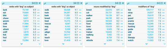
Figure 1.
WS columns for dog in the corpus English Web 2021 (enTenTen21).
While collocation analysis can provide valuable insights into a term’s semantic behavior, it cannot provide all the information needed to define a term. For instance, knowing that glyphosate commonly modifies resistance and frequently serves as the subject of the verb use is not sufficient. Additional types of semantic information are also needed to create its definition.
Syntactic co-occurrence should be complemented with an analysis of semantic co-occurrence. Two words are semantic co-occurrents if they establish a semantic relation in a given linguistic context (hyponymy, meronymy, cause, etc.) [28]. Semantic co-occurrents can be identified by querying corpora with knowledge patterns or lexico-syntactic patterns that convey a specific semantic relation [29,30]. For example, the knowledge pattern “x and other y” (e.g., “glyphosate and other pesticides”) conveys a hyponymic relation between x (glyphosate) and y (pesticide). The conceptual information extracted with semantic co-occurrence is generally more useful for definition writing than syntactic co-occurrence. However, a major limitation is the need for large corpora to obtain meaningful results, coupled with the challenge of filtering out significant noise [30,31]. Noise can arise because knowledge patterns may not consistently express the expected semantic relation. Moreover, they can be polysemic since they can express more than one semantic relation. Additionally, the effectiveness of knowledge patterns varies across different knowledge domains and genres [32].
The use of knowledge patterns for querying corpora can also be time-consuming if not automated. Unfortunately, most of the knowledge-pattern-based applications that have been designed for terminologists (or linguists in general), such as TerminoWeb [33], Caméleon [34], or WWW2REL [35], are no longer freely available. To the best of our knowledge, the only user-friendly tools currently available are Corpógrafo (https://www.linguateca.pt/corpografo/) (accessed on 2 March 2025) [36] and the EcoLexicon Semantic Sketch Grammar for Sketch Engine (ESSG) (http://ecolexicon.ugr.es/essg) (accessed on 2 March 2025) [37,38]. The ESSG allows for the extraction of semantic relations in English and French from a corpus by using WSs, as proposed in this paper for contextonym extraction. However, these tools are limited to a small number of semantic relations and languages, which means that employing semantic co-occurrence remains a time-consuming endeavor for many terminologists. As will be explained later, it is possible to configure a corpus in Sketch Engine to obtain syntactic, semantic, and contextonymic WSs in the same page.
Given the limitations associated with these two types of co-occurrence, we suggest adopting surface co-occurrence for extracting semantic information to aid in the creation of terminological definitions. Two words are considered surface co-occurrents if they appear in the same linguistic context, regardless of whether or not they are syntactically or semantically related [25]. For example, in “As the severity of the deficiency increases, chlorosis spreads to older leaves, which turn white and dry”, the terms chlorosis and deficiency are surface co-occurrents. Just as frequent syntactic co-occurrents are called collocations, we propose the term contextonym for those words that recurrently appear in the same linguistic context. The only limit for considering two terms contextonyms is the window size or predefined number of words between them. Crossing sentence and paragraph boundaries can be optionally permitted.
Since the contextonyms of a term tend to highlight its most relevant semantic characteristics [20], contextonym extraction can be helpful for definition writing. For instance, the analysis of the most frequent contextonyms of fungicide in an Agriculture corpus (i.e., application, control, disease, crop, resistance) shows that the most salient semantic features of fungicide in an agronomical context are that the application of fungicide allows for the control of certain diseases in crops, but some pathogens can develop resistance to them [28].
Contextonymy is not a transitive relation (e.g., the fact that chair is a contextonym of table and that back is a contextonym of chair does not imply that back is a contextonym of table), nor is it a symmetric relation (e.g., the fact that fire is a contextonym of lighter does not necessarily imply that lighter is a contextonym of fire). In addition, contextonyms, unlike hypernyms or synonyms, do not necessarily belong to the same word class (e.g., the verb sit can be a contextonym of the noun chair) [20].
It goes without saying that contextonyms are not universal and vary according to different contextual parameters, which can be thematic, cultural, temporal, etc. [16]. For example, the contextonyms of chlorine in an Air Quality Management corpus (ozone, stratosphere, CFC, depletion, etc.) describe it as a contributor to stratospheric ozone depletion, whereas its contextonyms in a Water Treatment corpus (water, disinfection, chlorination, kill, etc.) highlight its role as a water disinfectant [9]. For this reason, the corpus that is compiled should be in accordance with the contextual constraints of the definitions.
Although the results of a contextonym extraction must be interpreted (which could be streamlined with the use of a generative artificial intelligence tool [39]), contextonymy analysis is valuable because it can yield relevant insights even from smaller corpora, unlike semantic co-occurrence methods. Compared to knowledge patterns, the main advantage of contextonym analysis is that it can potentially uncover a wider range of semantic information without the need to manually define the relations to be captured.
San Martín [9] demonstrated that contextonym analysis in the form of a WS (Figure 2) is a valuable method for informing terminological definition writing. However, his approach relied on a window size of 44 words, based on a pilot study of somewhat limited scope [40]. In this paper, we present a more comprehensive study aimed at identifying the optimal window size of a WS column for contextonym analysis.
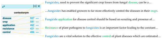
Figure 2.
Contextonymic WS of the term fungicide in an Agriculture corpus and associated concordances [28].
3. Materials and Methods
The first step in our study involved compiling a single-domain corpus on Agriculture, totaling approximately 8 million words. Twenty agricultural terms were then selected from the most frequent in the corpus. For each term, definitions were obtained from various resources to create a corpus of definitions, which was used as a gold standard. Once both corpora were processed, the list of the most frequent lemposes for each term was extracted from its definitions. In Sketch Engine, a lempos is a unit that combines a lemma and part-of-speech. It allows for distinguishing between homographs belonging to different word classes. Thus, for example, crop (noun) and crop (verb) are considered separate units. The contextonyms (in lempos format) according to the different window sizes were also extracted for each term from the Agriculture corpus.
For each term, the frequency list extracted from the definition corpus was compared to the contextonym lists on two metrics: cosine similarity, and the precision of the contextonym lists with respect to the frequency list of the definition corpus. This comparison determined which contextonym list was most similar to the frequency list of the definition corpus. For example, for monoculture, we compared a frequency list extracted from its definitions with its contextonyms, obtained with different context windows (5, 10, 20, etc.). This operation was repeated for each term. The optimal context window was the one that yielded the best average of normalized cosine similarity and precision. Figure 3 visually represents the methods used in this research.
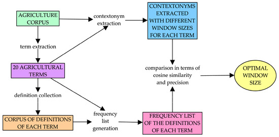
Figure 3.
Visual representation of the methods used in this research.
It is important to note that the objective of this paper is not to validate the usefulness of contextonyms or a contextonym-based WS for terminological definition writing—this is taken as given for the purposes of our study. Our main objective is thus to find the most useful configuration for definition writing (i.e., the most similar to the frequency list extracted from the definitions). It is also important to note that, although each term might have its own optimal contextonymic configuration, our goal is to identify a single configuration that will be broadly applicable and useful across a wide range of different terms.
The novelty of this study is that it is the first to systematically determine the optimal context window for extracting co-occurrence data to aid terminological definition writing. Methodologically, to achieve this objective, we introduce the novel approach of comparing contextonyms to a corpus of definitions, allowing us to evaluate the performance of different window sizes and identify the optimal one.
3.1. Agriculture Corpus
In order to minimize the interference caused by polysemy and contextual variation, we limited our experiment to a single specialized domain: Agriculture. The corpus totaled 8,254,771 words and included specialized texts written in English, such as the following:
- Theoretical and practical documents on Agriculture published by the Food and Agriculture Organization (FAO) and various national and regional governments in English-speaking countries. These texts were manually extracted from the web to ensure their quality [29.6%].
- Specialized monographs and encyclopedias on Agriculture. These texts were manually extracted from the digital version of these resources [30.6%].
- Scientific articles from the open-access journals Frontiers in Agriculture, International Journal of Agronomy, and Agronomy. These texts were automatically scraped using a Python 3.13 script [30.9%].
- Articles from Wikipedia, manually selected to belong to the field of Agriculture. These texts were automatically scraped using a Python 3.13 script [8.8%].
3.2. Selection of Terms and Compilation of the Definition Corpus
The next step involved selecting the terms for analysis. Terms were extracted from the Agriculture corpus using TermoStat Web 3.0 [41]. The focus was on simple nouns, two-word complex nominals, and verbs. The 50 most frequent candidate terms per category were retained.
The definitions of each of the terms were then collected from 173 paper and electronic resources. The list of sources can be found in https://doi.org/10.5281/zenodo.15002751. Definitions were only retained if they were sourced from resources specifically focused on Agriculture or any of its subdomains, or, in cases involving multidomain resources, if the term or definition was explicitly labeled as pertaining to Agriculture or any of its subdomains.
Based on the information in the definitions, interdomain polysemic terms were eliminated and the terms were divided into entities, processes/activities, or attributes. The five terms with the most definitions in each category (simple noun entity, simple noun process, complex noun entity, and complex noun process) were selected. At this stage, verbs and attribute-type nouns were excluded because not enough definitions were found for them.
Table 1 shows the five terms selected for each category, along with the number of definitions extracted and their word count. In total, the definition corpus consisted of 504 definitions and 15,570 words.

Table 1.
List of 20 terms with their type, the number of definitions, and definition word count.
All the definitions were included in an XML-tagged corpus. The definitions of each term were included within a <term> tag and each definition was included within a <def> subtag, which allowed us to analyze the definitions of each term separately in Sketch Engine.
3.3. Corpus Processing
To minimize interference from geographic and non-geographic orthographic variants, we normalized both corpora using a Python 3.13 script that automatically converted the texts to U.S. spelling. This script was based on a list of words that have British and U.S. spelling variants (e.g., all occurrences of “fibre” became “fiber”). Additionally, the script removed hyphens from words beginning with a prefix (e.g., all instances of “micro-organism” became “microorganism”).
As for the Agriculture corpus, all the bibliographic reference lists were manually removed because preliminary contextonym extraction showed that these lists introduced noise. Texts that were scraped from the web had already been extracted without their reference lists. The information in Section 3.1 regarding the size and composition of the corpus reflects this treatment of the corpus.
In regard to the definition corpus, all metalinguistic formulas were eliminated from the definitions, such as “This term refers to…” or “Type of…”, in order to prevent words not semantically related to the defined term (e.g., term, type or refer) from being overrepresented. Moreover, given that the definition corpus functioned as a gold standard and was of manageable size, all obvious spelling mistakes were manually corrected. Finally, once the corpus was compiled, the lemmatization and part-of-speech tagging were manually corrected in the vertical file, namely, the lemmatized and part-of-speech tagged corpus file generated by Sketch Engine. For example, in “The cultivation of marine or freshwater aquatic plants”, Sketch Engine (using TreeTagger) incorrectly tagged marine as a noun rather than an adjective, which was then manually corrected.
In both the frequency list from the definition corpus and the extraction of contextonyms, only nouns, verbs, and adjectives were considered, as these are the most semantically significant part-of-speech categories. Adverbs were excluded because their informative role in definition writing is likely limited. However, this decision was based on preliminary assessments, and further study is required to fully understand the impact of adverbs in this context.
A stop list was created and applied to the results obtained from both the list of definitions and the contextonym extraction. This stop list included common words whose semantic content was regarded as too general to be useful for definition writing (be, different, do, due, few, have, least, less, make, many, more, most, much, only, other, same, such). Recognizing the subjective nature of this selection, it is important to note that in a real context of contextonym usage, a terminologist could easily modify the stop list.
3.4. Contextonymic Sketch Grammar
3.4.1. WS Generation in Sketch Engine
The generation of WS in Sketch Engine relies on the matching of patterns encoded as rules expressed in CQL language [42]. A CQL rule consists of tokens in the form of attributes (part-of-speech tag, lemma, word form, etc.) and values, combined with regular expressions. For example, the rule [tag="J.*"] [tag="N.*"] [lemma="development"] matches concordances where the lemma development is preceded by a noun and an adjective (e.g., mobile software development, longitudinal resource development, and digital library development).
A CQL rule designed for WS generation identifies the position of the words to be extracted as the WS results. For example, the rule 1:[tag="V.*"] [tag="J.*"]? 2:[tag="N.*"] extracts a verb (1:) that is followed by an optional adjective and a noun (2:). Inversely, it also allows for the extraction of a noun (2:) preceded by an optional adjective, which in turn is preceded by a verb (1:). In this case, Sketch Engine identifies the matches of the rule (a verb followed by an optional adjective and a noun) in the corpus, and then extracts the verb and the noun from each matched concordance. It is important to note that WS results are limited to single words.
For WS generation, the CQL rules designed to identify the same relation are grouped into a gramrel (for grammatical relation). Each gramrel can produce one or more WS columns (normally two: one relation and its reverse). The collection of gramrels that generate a WS is referred to as a sketch grammar. For instance, the gramrel in Sketch Engine’s default sketch grammar that identifies the relation between the object of a sentence and its verb generates two WS columns (“objects of “X”” and its reverse “verbs with “X” as object”) by means of three rules (Figure 4). The first rule identifies the object–verb relation in the active voice and the other two in the passive voice (one without the verb to be and the other with it).
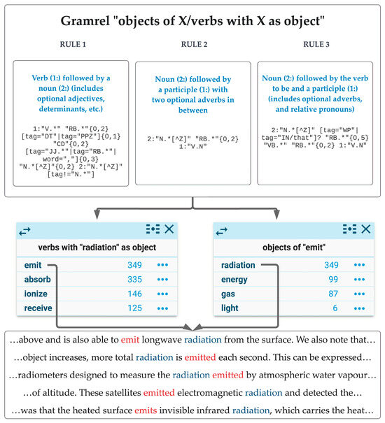
Figure 4.
The “objects of “X”/verbs with “X” as object” gramrel in the default English sketch grammar with an example from the EcoLexicon English Corpus.
3.4.2. Parameters of the Contextonymic WS
The criteria for extracting contextonyms are varied and can include multiple parameters [25]. In what follows, we focus on those parameters that are configurable for a contextonymic WS, such as different window sizes, limitation to sentence or paragraph boundaries, sorting results by frequency or association score, the selection of only specific word classes, and the use of a stop list.
As for the context window, we created 17 different contextonymic gramrels with different symmetric context windows (5, 10, 20, 30, 40, 50, 75, 100, 150, 200, 250, 300, 400, 500, 1000, 2000, and 3000 tokens). Tokens include punctuation and digits. Our approach mirrors that of bag-of-words models in distributional semantics since it focuses on the presence of words within a certain span, but does not consider word order or the distance from the keyword, which is not possible with WSs.
Although the use of asymmetric windows (i.e., allowing different numbers of tokens before and after the keyword) was technically feasible, we decided to leave the comparison of symmetric and asymmetric windows for future research. All gramrels were configured to cross sentence boundaries, except for an 18th contextonymic gramrel, which only extracted contextonyms in the same sentence. We included a gramrel that was constrained to not cross sentence boundaries to assess whether it yields better results compared to those not limited to the sentence level. We did not take paragraph boundaries into account because paragraphs were not tagged in our corpus.
Although different association scores could be useful for contextonym extraction, our sorting parameters were limited to those available with WSs, namely by raw frequency and by the logDice association score [27]. LogDice is an association score that aims at detecting collocations, which is the typical purpose of WSs. This purpose diverges from that of contextonym extraction. Nevertheless, it was included in our study because it is the sorting criterion for WS results by default in Sketch Engine. As for the frequency lists from the definition corpus, they were ordered by the number of definitions in which each term appears.
Finally, as previously mentioned, both in the frequency lists of the definition corpus and in the extractions of contextonyms from the Agriculture corpus, only nouns, verbs, and adjectives were considered. A stop list was also created and applied to the results from both the frequency list from the definitions and the contextonym extractions.
3.4.3. Creation of the Contextonymic Sketch Grammar
Contextonymic gramrels were created for each window size (5 tokens, 10 tokens, 20 tokens, etc.), as well as a version where contextonym extraction was restricted to sentence boundaries.
Firstly, in the form of an m4 macro, a contextonym was defined as any noun (common or proper), any adjective, or any verb, provided that its lemma does not match any lemmas on the stop list and is not a digit (Table 2).
Table 2.
M4 macro defining a contextonym.
Next, the gramrels for each window size were encoded. For example, Table 3 explains the five-word window contextonym gramrel.
Table 3.
Gramrel for the extraction of contextonyms in a five-token window size.
The structure of the gramrel that limits contextonym detection within the sentence is explained in Table 4.
Table 4.
Gramrel for the extraction of contextonyms bounded to sentence limits.
3.4.4. Contextonym Extraction for Complex Nominals
Because of the technical limitations in generating WSs from multiword terms, we adapted our approach to the 10 complex nominals on our list. For each complex nominal (e.g., sustainable agriculture), we created a modified version of the corpus where all instances of the complex nominal were replaced with a concatenated version of the term (e.g., sustainable agriculture). Additionally, both components of the complex nominal were added to the specific stop list for that term (e.g., sustainable and agriculture for sustainable agriculture) to avoid obtaining them as contextonyms.
3.5. Analysis Methods
For each term, we compared the first 42 lemposes of each list of contextonyms ordered by frequency and logDice score with the frequency list extracted from the definition corpus of each term (frequency was calculated as the number of definitions in which the lempos appeared). If the lempos was not present in the list of frequencies extracted from the definition corpus (because it did not appear in at least two definitions), a frequency of 0 was attributed to it. By way of example, Table 5 shows the 42 lemposes that were used to compare the five-token window contextonyms of pasture ordered by frequency and the frequency list from the definition corpus.
Table 5.
Comparison of pasture (context window of five tokens vs. frequency list from definitions).
We selected 42 results as it is the default number of results displayed in a WS column by Sketch Engine when users click the button that shows more data once. We decided not to use 12 (the default number of results before clicking to see more results) because this number provides too few results. Clicking on the button that shows more results twice increases the list to 72 results. However, we did not use 72 because only six of our analysis terms had more than 72 results in the frequency list from the definition corpus that met the inclusion criteria—being a noun, adjective or verb; appearing in two or more different definitions; not being on the stop list; and not being the defined term or part of it (in the case of complex nominals).
Since the frequency or logDice score of each of the elements of a list forms a vector, as well as the frequency of the elements of the frequency list of definitions, we quantified their similarity by cosine similarity. Cosine similarity is the most common measurement used in distributional semantics [23]. In the case of positive numbers (which was our case), it ranges from 0 (lowest similarity) to 1 (highest similarity). Using cosine similarity allowed us to compare whether the frequency or score associated with the contextonym results resembled the frequency of occurrence of the terms in the definitions.
To identify the optimal contextonymic window size, we calculated the average of the normalized cosine similarity and precision (percentage of results in the contextonyms list also present in the frequency list of the definition corpus). Precision was included to provide more weight to the presence or absence of the terms from the frequency list of the definition corpus among the contextonyms, since cosine similarity does not sufficiently penalize absences.
4. Results
4.1. Frequency vs. logDice Score
First, we evaluated the performance of all contextonym extractions depending on whether the contextonyms were ordered by frequency or by score by comparing them with the frequency list extracted from the definition corpus of each term. As shown in Table 6 and Table 7, in all cases, whether considering precision or cosine similarity, frequency provided better results in all context windows. Since ordering results by frequency consistently yielded better outcomes than ordering results by logDice score, the rest of the paper solely focuses on frequency-sorted results.
Table 6.
Average precision of each context window with results ordered by frequency and by logDice score.
Table 7.
Average cosine similarity of each context window with results ordered by frequency and by logDice score.
4.2. Frequency-Ordered Results
4.2.1. Results According to Cosine Similarity
Table 8 displays the cosine similarity results for each context window by term. The last row presents the mean average for each context window. Each term exhibited a different optimal context window in terms of cosine similarity. However, the 100-token window emerged as the average best context window across all terms, with an average cosine similarity of 0.644. Notably, the poorest results were associated with the smallest context window (i.e., the five-token window). Additionally, context windows exceeding 100 tokens showed a decline in performance as the window size increased.
Table 8.
Frequency-ordered results according to cosine similarity, with green indicating higher values and red representing lower values.
4.2.2. Results According to Precision
Table 9 shows the precision results for each contextonym context window by term. The last row presents the mean average for each context window. Each term has a different optimal context window in terms of cosine similarity. However, the 30-token window emerged as the average best context window across all terms with a precision of 40.8%. The lowest precision was that of the 2000-token window.
Table 9.
Frequency-ordered results according to precision, with green indicating higher values and red representing lower values.
4.2.3. Combined Results of Cosine Similarity and Precision
As shown above, the optimal context window differs depending on the evaluation metric. Based on cosine similarity, the best window size is 100 tokens, while in terms of precision, it is 30 tokens. Consequently, to find the optimal context window for our contextonymic sketch grammar, we calculated the average of the cosine similarity and precision, both normalized to a range of 0 to 1 using min–max scaling (Table 10). The results indicate that the optimal context window for extracting contextonyms for writing terminology definitions is 50 tokens.
Table 10.
Normalized average of cosine similarity and precision, with green indicating higher values and red representing lower values.
4.3. Proposed Contextonymic Sketch Grammar
The gramrel with the optimal window context (i.e., 50 tokens) is reproduced in Table 11.
Table 11.
Fifty-token contextonymic sketch grammar.
To use this contextonymic sketch grammar in Sketch Engine with a new corpus, the user should follow these steps:
- Click on the “New corpus” button in the top right-hand corner of the Sketch Engine home page.
- Enter the corpus name, type and language (English). Then, click “Next”.
- Choose to create the corpus from web documents or local files. Click “Next” to proceed.
- Expand the “Expert settings” drop-down menu and select the “Sketch grammar” option.
- Click on the cross to add a sketch grammar.
- Enter a name for the sketch grammar.
- Paste the contents of the sketch grammar into the provided space. It is possible to paste the default English sketch grammar, as well as the ESSG sketch grammar, followed by the contextonymic one in order to create WSs that contain all three types on the same page.
- Click “Save and compile” to complete corpus creation.
- When using the WS function, the contextonymic WS column will be available.
4.4. Example of a Contextonymic Word Sketch
As an example of the usefulness of the contextonymic word sketch as a source of definitional information, Figure 5 presents the results of applying the contextonymic word sketch (with a 50-token window size) to the term herbicide in the Agriculture corpus used in this study. By examining the first 10 contextonyms of herbicide in the corpus, along with some of its corresponding concordance lines, it becomes evident that key semantic features of the term within the domain of Agriculture include that herbicides are applied to crops and soil to kill or inhibit the growth of weeds, providing efficient weed control by targeting specific plants, though repeated use can lead to resistance in weed species. Notably, these contextonyms also highlight the conceptual frame in which herbicide participates within the domain of Agriculture, which can be called weed control. For space reasons, this example is limited to 10 results. However, the terminologist would typically need to consult more than 10 contextonyms to extract the most relevant definitional information for the term being defined.
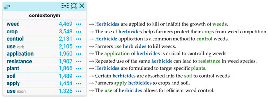
Figure 5.
The first 10 contextonyms of herbicide in the Agriculture corpus, along with an explanation of their relationship to it (obtained through analysis of the corresponding concordance lines).
The terminologist must evaluate the information gathered through contextonym analysis alongside information obtained from other methods, such as consulting specialized texts, reviewing existing definitions from other resources, or conducting corpus analysis based on knowledge patterns. This combined analysis helps determine which features should be included in the definition of herbicide.
5. Discussion
Our study systematically determines that optimal context window for extracting co-occurrence data to aid terminological definition writing is 50 tokens. While the experiment was conducted using an Agriculture corpus, the methodology itself is designed to be generalizable to other domains. The combination of contextonym extraction and comparison with a definition corpus provides an empirical and reproducible framework that can be applied to different fields.
The use of cosine similarity and precision as evaluation metrics ensures that the results are based on quantitative, objective measures, rather than subjective interpretation. Additionally, by testing multiple context window sizes and selecting the most effective one, our study avoids the arbitrary selection of parameters, reinforcing the robustness of the findings.
However, we acknowledge that this study was conducted on a single-domain dataset, and additional validation on corpora from other fields would further confirm the method’s applicability. Future research will apply this approach to datasets from different disciplines, such as Medicine and Law, to assess its cross-domain reliability. Additionally, testing the methodology in different languages will help determine whether the context window needs to be adapted for each language. Despite these limitations, our results provide a strong foundation for contextonym-based terminological definition writing and establish a replicable framework for further research.
While this study identifies the optimal parameters for extracting contextonyms to aid definition writing, the practical application of these findings requires further refinement. In particular, guidelines should be developed to help terminologists systematically interpret and integrate contextonym analysis into their workflow. Defining the best practices for filtering and prioritizing contextonyms will ensure their effective use, allowing for terminologists to faithfully capture conceptualizations in terminological definitions.
Other future work to address the limitations of this study includes the exploration of the potential benefits of including adverbs in our analysis and whether asymmetric windows yield better results than symmetric ones. Finally, another research avenue involves testing contextonym extraction outside the Sketch Engine framework. This approach would allow us to experiment with parameters that are not feasible with WSs, such as using different association scores or assigning different weights to contextonyms based on their distance from the keyword.
6. Conclusions
Our proposal of contextonym analysis for writing terminological definitions fills a gap in terms of methods available for this task, since current guidelines on how to select the information to include in a definition are limited to the specification of necessary and sufficient characteristics. Contextonym extraction using WSs is a user-friendly method to obtain potentially useful semantic information for defining terms from any user-owned corpus. It offers an objective method to determine the relevance of semantic features to be included in a definition.
Compared to collocations and knowledge patterns, contextonym analysis captures a wider range of semantically relevant information. As we have seen, it can even help identify the frame in which the term participates and other terms that participate in the same frame. This makes contextonym analysis a valuable complement to other kinds of co-occurrence analysis. This study has found that the optimal context window for extracting contextonyms in the form of a WS in English to inform terminological definition writing was 50 tokens, and that these contextonyms should be ranked by frequency.
Contextonym analysis helps to create contextualized definitions that provide more relevant information for users. In this sense, contextonym analysis allows for the practical implementation of the FTDA, as it makes it possible to access how a term is conceptualized within specific contexts. As a consequence, the terminologist can more accurately represent the contextual variation of terms in definitions.
Finally, unlike most distributional semantic applications that require advanced programming skills by the user, this paper presents a user-friendly tool. The contextonymic sketch grammar can be easily applied by terminologists to any user-owned corpus. Moreover, integrating this function into Sketch Engine enhances its practicality by incorporating contextonym analysis into a widely used corpus tool that already offers valuable features for definition writing and terminology work, such as syntactic and semantic word sketches, concordances, and terminology extraction.
Funding
This research was funded by Canada’s Social Sciences and Humanities Research Council, grant number 430-2023-0248, and Spain’s Ministry of Science and Innovation, grant number PID2020-118369GB-I00.
Data Availability Statement
The original contributions presented in this study are included in the article. Further inquiries can be directed to the corresponding author.
Acknowledgments
The author thanks Professor Dirk Speelman for his valuable insights before the writing of this article.
Conflicts of Interest
The author declares no conflicts of interest.
Abbreviations
The following abbreviations are used in this manuscript:
| ESSG | EcoLexicon Semantic Sketch Grammar |
| FTDA | Flexible Terminological Definition Approach |
| WS | Word sketch |
References
- Suonuuti, H. Guide to Terminology; Tekniikan Sanastokeskus ry: Helsinki, Finland, 1997; ISBN 952-9794-14-2. [Google Scholar]
- Pavel, S.; Nolet, D. Précis de Terminologie; Bureau de la traduction: Gatineau, QC, Canada, 2001; ISBN 0-660-61616-5. [Google Scholar]
- Dubuc, R. Manuel pratique de Terminologie; Linguatech: Brossard, QC, Canada, 2002; ISBN 978-2-920342-42-2. [Google Scholar]
- Kockaert, H.J.; Steurs, F. (Eds.) Handbook of Terminology; John Benjamins: Amsterdam, The Netherlands; Philadelphia, PA, USA, 2015; ISBN 978-90-272-5777-2. [Google Scholar]
- ISO/TC 37/SC 1 ISO 704:2022; Terminology Work—Principles and Methods. ISO: Geneva, Switzerland, 2022.
- Vézina, R.; Darras, X.; Bédard, J.; Lapointe-Giguère, M. La Rédaction de Définitions Terminologiques; Office québécois de la langue française: Montréal, QC, Canada, 2009; ISBN 978-2-550-55484-4. [Google Scholar]
- Fargas, F.X. La Definició Terminològica; Termcat, Ed.; Eumo: Barcelona, Spain, 2009; ISBN 978-84-9766-327-4. [Google Scholar]
- Temmerman, R. Towards New Ways of Terminology Description: The Sociocognitive Approach; John Benjamins: Amsterdam, The Netherlands; Philadelphia, PA, USA, 2000; ISBN 978-90-272-2326-5. [Google Scholar]
- San Martín, A. A Flexible Approach to Terminological Definitions: Representing Thematic Variation. Int. J. Lexicogr. 2022, 35, 53–74. [Google Scholar] [CrossRef]
- Seppälä, S. An Ontological Framework for Modeling the Contents of Definitions. Terminology 2015, 21, 23–50. [Google Scholar] [CrossRef][Green Version]
- Evans, V. Cognitive Linguistics: A Complete Guide; Edinburgh University Press: Edinburgh, UK, 2019; ISBN 978-1-4744-0521-8. [Google Scholar]
- Kecskes, I. The Socio-Cognitive Approach to Communication and Pragmatics; Perspectives in Pragmatics, Philosophy & Psychology; Springer International Publishing: Cham, Switzerland, 2023; Volume 33, ISBN 978-3-031-30159-9. [Google Scholar]
- Evans, V. A Unified Account of Polysemy within LCCM Theory. Lingua 2015, 157, 100–123. [Google Scholar] [CrossRef]
- Hanks, P. How Context Determines Meaning. In Computational Phraseology; Corpas Pastor, G., Colson, J.-P., Eds.; John Benjamins: Amsterdam, The Netherlands, 2020; Volume 24, pp. 297–310. ISBN 978-90-272-0535-3. [Google Scholar]
- Faber, P.; León-Araúz, P. From Specialized Knowledge Frames to Linguistically Based Ontologies. Appl. Ontol. 2024, 19, 23–45. [Google Scholar] [CrossRef]
- San Martín, A. Contextual Constraints in Terminological Definitions. Front. Commun. 2022, 7, 885283. [Google Scholar] [CrossRef]
- Cruse, A. Meaning in Language; Oxford University Press: Oxford, UK, 2011; ISBN 978-0-19-955946-6. [Google Scholar]
- Freixa, J.; Fernández-Silva, S. Terminological Variation and the Unsaturability of Concepts. In Multiple Perspectives on Terminological Variation; Drouin, P., Francœur, A., Humbley, J., Picton, A., Eds.; John Benjamins: Amsterdam, The Netherlands; Philadelphia, PA, USA, 2017; pp. 155–180. ISBN 978-90-272-6543-2. [Google Scholar]
- San Martín, A. La Representación de la Variación Contextual Mediante Definiciones Terminológicas Flexibles. Ph.D. Thesis, University of Granada, Granada, Spain, 2016. [Google Scholar]
- Lenci, A. Distributional Models of Word Meaning. Annu. Rev. Linguist. 2018, 4, 1065975714. [Google Scholar] [CrossRef]
- Ji, H.; Ploux, S.; Wehrli, E. Lexical Knowledge Representation with Contexonyms. In Proceedings of the 9th MT summit Machine Translation, New Orleans, LA, USA, 23–27 September 2003; pp. 194–201. [Google Scholar]
- Ji, H.; Ploux, S. Automatic Contexonym Organizing Model (ACOM). In Proceedings of the 25th Annual Conference of the Cognitive Science Society; Alterman, R., Kirsch, D., Eds.; Psychology Press: Boston, MA, USA, 2003; pp. 622–627. [Google Scholar]
- Ji, H.; Gaiffe, B.; Choo, H. Selecting Target Word Using Contexonym Comparison Method. In Human Interface and the Management of Information. Methods, Techniques and Tools in Information Design; Smith, M.J., Salvendy, G., Eds.; Lecture Notes in Computer Science; Springer: Berlin/Heidelberg, Germany, 2007; Volume 4557, pp. 463–470. ISBN 978-3-540-73344-7. [Google Scholar]
- Evert, S. Corpora and Collocations. In Corpus Linguistics: An International Handbook (Volume 2); Lüdeling, A., Kytö, M., Eds.; De Gruyter: Berlin, Germany, 2009; pp. 1212–1248. ISBN 978-3-11-021388-1. [Google Scholar]
- Bartsch, S. Structural and Functional Properties of Collocations in English: A Corpus Study of Lexical and Pragmatic Constraints on Lexical Co-Occurrence; Gunter Narr Verlag: Tübingen, Germany, 2004; ISBN 978-3-8233-5893-0. [Google Scholar]
- Kilgarriff, A.; Baisa, V.; Bušta, J.; Jakubíček, M.; Kovář, V.; Michelfeit, J.; Rychlý, P.; Suchomel, V. The Sketch Engine: Ten Years On. Lexicography 2014, 1, 7–36. [Google Scholar] [CrossRef]
- Rychlý, P. A Lexicographer-Friendly Association Score. In Proceedings of the Second Workshop on Recent Advances in Slavonic Natural Language Processing, RASLAN 2008, Karlova Studánka, Czech Republic, 5–7 December 2008; Masaryk University: Brno, Czech Republic, 2008. [Google Scholar]
- San Martín, A.; Trekker, C. Adapting Word Sketches for Specialized Knowledge Extraction. In Proceedings of the 14th International Conference of the Asian Association for Lexicography (ASIALEX), Jakarta, Indonesia, 12–14 June 2021; ASIALEX: Jakarta, Indonesia, 2021; pp. 64–87. [Google Scholar]
- Marshman, E. Knowledge Patterns in Corpora. In Theoretical Perspectives on Terminology: Explaining Terms, Concepts and Specialized Knowledge; Faber, P., L’Homme, M.-C., Eds.; John Benjamins: Amsterdam, The Netherlands; Philadelphia, PA, USA, 2022; pp. 291–310. ISBN 978-90-272-5778-9. [Google Scholar]
- Meyer, I. Extracting Knowledge-Rich Contexts for Terminography. A Conceptual and Methodological Framework. In Recent Advances in Computational Terminology; Bourigault, D., Christian, C., L’Homme, M.-C., Eds.; John Benjamins: Amsterdam, The Netherlands, 2001; pp. 279–302. ISBN 978-1-58811-016-9. [Google Scholar]
- Bowker, L. Lexical Knowledge Patterns, Semantic Relations, and Language Varieties: Exploring the Possibilities for Refining Information Retrieval in an International Context. Cat. Classif. Q. 2003, 37, 153–171. [Google Scholar] [CrossRef]
- Condamines, A. How the Notion of “Knowledge Rich Context” Can Be Characterized Today. Front. Commun. 2022, 7, 824711. [Google Scholar] [CrossRef]
- Barrière, C.; Agbago, A. TerminoWeb: A Software Environment for Term Study in Rich Contexts. In Proceedings of the 3rd International Conference on Terminology, Standardization and Technology Transfer (TSTT 2006), Beijing, China, 25–26 August 2006; China National Institute of Standardization: Beijing, China, 2006. [Google Scholar]
- Aussenac-Gilles, N.; Jacques, M.-P. Designing and Evaluating Patterns for Relation Acquisition from Texts with Caméléon. Terminology 2008, 14, 45–73. [Google Scholar] [CrossRef][Green Version]
- Halskov, J.; Barrière, C. Web-Based Extraction of Semantic Relation Instances for Terminology Work. Terminology 2008, 14, 20–44. [Google Scholar] [CrossRef]
- Maia, B.; Matos, S. Corpógrafo V.4—Tools for Researchers and Teachers Using Comparable Corpora. In Proceedings of the LREC 2008 Workshop on Comparable Corpora; Zweigenbaum, P., Gaussier, É., Fung, P., Eds.; ELRA: Marrakesh, Morocco, 2008; pp. 79–82. [Google Scholar]
- León-Araúz, P.; San Martín, A. The EcoLexicon Semantic Sketch Grammar: From Knowledge Patterns to Word Sketches. In Proceedings of the LREC 2018 Workshop “Globalex 2018—Lexicography & WordNets”; Kerneman, I., Krek, S., Eds.; Globalex: Miyazaki, Japan, 2018; pp. 94–99. [Google Scholar]
- San Martín, A.; Trekker, C.; León-Araúz, P. Repérage automatisé de l’hyponymie dans des corpus spécialisés en français à l’aide de Sketch Engine. Terminology 2022, 28, 264–298. [Google Scholar] [CrossRef]
- San Martín, A. What Generative Artificial Intelligence Means for Terminological Definitions. In Proceedings of the 3rd International Conference on Multilingual Digital Terminology Today (MDTT 2024), Granada, Spain, 27–28 June 2024; CEUR-WS: Granada, Spain, 2024. [Google Scholar]
- San Martín, A. KWIC Corpora as a Source of Specialized Definitional Information: A Pilot Study. In Actes du CEC-TAL’2013; Zaghouani, W., Ed.; Université du Québec à Montréal: Montreal, QC, Canada, 2014. [Google Scholar]
- Drouin, P. Term Extraction Using Non-Technical Corpora as a Point of Leverage. Terminology 2003, 9, 99–115. [Google Scholar] [CrossRef]
- Jakubíček, M.; Kilgarriff, A.; McCarthy, D.; Rychlý, P. Fast Syntactic Searching in Very Large Corpora for Many Languages. In Proceedings of the 24th Pacific Asia Conference on Language, Information and Computation; Otoguro, R., Ishikawa, K., Umemoto, H., Yoshimoto, K., Harada, Y., Eds.; Institute of Digital Enhancement of Cognitive Processing, Waseda University: Sendai, Japan, 2010; pp. 741–747. [Google Scholar]


Disclaimer/Publisher’s Note: The statements, opinions and data contained in all publications are solely those of the individual author(s) and contributor(s) and not of MDPI and/or the editor(s). MDPI and/or the editor(s) disclaim responsibility for any injury to people or property resulting from any ideas, methods, instructions or products referred to in the content. |
© 2025 by the author. Licensee MDPI, Basel, Switzerland. This article is an open access article distributed under the terms and conditions of the Creative Commons Attribution (CC BY) license (https://creativecommons.org/licenses/by/4.0/).