Detecting Potential Investors in Crypto Assets: Insights from Machine Learning Models and Explainable AI

Abstract

This study explores the characteristics of individual investors in crypto asset markets using machine learning and explainable artificial intelligence (XAI) methods. The primary objective was to identify the most effective model for predicting the likelihood of an individual investing in crypto assets in the future based on demographic, behavioral, and financial factors. Data were collected through an online questionnaire distributed via social media and personal networks, yielding a limited but informative sample. Among the tested models, Efficient Linear SVM and Kernel Naïve Bayes emerged as the most optimal, balancing accuracy and interpretability. XAI techniques, including SHAP and Partial Dependence Plots, revealed that crypto understanding, perceived crypto risks, and perceived crypto benefits were the most influential factors. For individuals with a high likelihood of investing, these factors had a strong positive impact, while they negatively influenced those with a low likelihood. However, for those with a moderate investment likelihood, the effects were mixed, highlighting the transitional nature of this group. The study’s findings provide actionable insights for financial institutions to refine their strategies and improve investor engagement. Furthermore, it underscores the importance of interpretable machine learning in financial behavior analysis and highlights key factors shaping engagement in the evolving crypto market.

1. Introduction

Investing in crypto assets has become one of the topics that has received a lot of attention in the financial world over the last decade. What started as a niche experiment with Bitcoins has quickly evolved into a global phenomenon, attracting investors of all kinds—from tech aficionados and speculators to institutional investors. This idea, first presented in 2008 as part of a proposal to solve the problem of double spending through peer-to-peer networks, is based on the use of a blockchain. As it is presented [1], the system records transactions using a proof-of-work algorithm, ensuring transparency, immutability, and security without the need to trust a third party. Crypto markets promise high returns but also carry extreme volatility and risk, putting them in a unique position compared to traditional investments such as stocks, bonds, or real estate [2].

Crypto assets present a unique combination of opportunities and risks. As a highly speculative asset class, they belong to a small part of a well-diversified portfolio [2]. Although many projects are likely to fail, some have the potential to reach high values and become a key part of the new blockchain economy. However, the scenario cannot be ruled out that the whole digital asset class will remain a short-lived fad, similar to the beanie babies of yore, which will eventually disappear from the financial scene and become a curiosity of the past.

Whatever the future fate of crypto assets, the sudden surge in activity, the extreme volatility, the high failure rate, and the high regulatory uncertainty point to the need for a structured framework for their valuation and understanding. It is crucial that investors and regulators develop a deeper understanding of the practical use cases for digital assets and establish regulatory guidelines that will both protect investors and foster innovation in this rapidly evolving space.

In this article, we will explore the probability of individuals investing in crypto assets in the future based on demographic, behavioral, and financial factors. Traditional methods for analyzing investor behavior often rely on linear assumptions and predefined variable relationships, which may not fully capture the complexity of decision-making in the crypto market. Given the diverse demographic, behavioral, and financial factors influencing investment choices, more flexible approaches are required. Machine learning models offer the advantage of detecting nonlinear patterns and interactions that might be overlooked in conventional analyses. Therefore, our research focuses on testing different machine learning and artificial intelligence models to determine which approach most accurately predicts the likelihood of investment in crypto assets. By leveraging advanced analytical techniques, we aim to provide deeper insights into the key determinants influencing investment decisions in this rapidly evolving field.

The findings of this study are particularly relevant for investment firms, as they offer valuable insights into the probability of individuals entering the crypto market. Understanding these predictive factors can help firms tailor their products and marketing strategies to align with the needs and preferences of potential investors. Additionally, by evaluating various models to identify the most effective one, firms can refine their risk assessment strategies and optimize their approach to engaging with emerging investor segments.

Our research is structured into several key sections. First, we will review existing literature and research on crypto asset investment behavior, forming the foundation for our analysis. In the methodology section, we will outline the data collection process, data preprocessing steps, and the construction of the final dataset used in our study. This will be followed by an analysis of the results, where we will present the models tested, their predictive performance, and their accuracy in estimating the likelihood of investment. In the discussion section, we will further examine the underlying constructs that drive individuals toward crypto investments, providing a comprehensive understanding of the decision-making process. These insights can serve as a valuable resource for investment firms seeking to better anticipate market trends. Finally, we will summarize our main findings and discuss the practical applications and potential future developments in this field.

2. Literature Review

The literature on artificial intelligence (AI) in the crypto asset segment is extensive. A significant part of the research focuses on the development of investment strategies for investing in crypto assets with artificial intelligence. For example, there is research [3] that presents AI algorithms to optimize cryptocurrency trading strategies, while in the book [4] the author explores how artificial intelligence helps overcome barriers to investing in Bitcoin. Additionally, the introduction of explainable artificial intelligence models that enable the optimization of asset allocation in crypto portfolios was also presented [5].

Based on the type of research we are conducting, our focus will be on providing an overview of crypto investors’ characteristics. Additionally, we will delve into some of the key differences between crypto investors and non-investors, which will offer a better understanding of the motivations and behavioral patterns in the context of digital asset investment.

Looking a bit more generally, investment behavior can be explained through several theoretical models that highlight the key factors influencing financial decision-making. One of the most established models is Prospect Theory, which suggests that individuals evaluate potential gains and losses asymmetrically, giving more weight to losses than to equivalent gains—a bias particularly relevant in highly volatile markets like crypto assets [6].

Additionally, the Theory of Planned Behavior (TPB) posits that investment intentions are shaped by attitudes, social influence, and perceived behavioral control, making it suitable for explaining how demographic and behavioral factors affect crypto investments [7].

A relevant study [8] builds on this framework by examining how behavioral factors influence investment behavior in the crypto asset market. Their research applies the Decomposed Theory of Planned Behavior, which extends TPB by incorporating additional constructs such as perceived usefulness and ease of use. Their findings highlight that subjective norms (social influence) and perceived behavioral control are significant predictors of crypto investment intentions, reinforcing the idea that behavioral factors play a crucial role in financial decision-making. This study provides a strong theoretical foundation for our research, supporting the need to include demographic and behavioral variables in our analysis.

Behavioral finance further emphasizes the role of psychological biases such as overconfidence, herd behavior, and anchoring, which can drive irrational investment decisions in speculative markets like cryptocurrencies [9].

In the context of digital assets, the Technology Acceptance Model (TAM) highlights how technological literacy and perceived usefulness of blockchain technology influence investment decisions [10].

A recent literature review [11] highlights increasing evidence of herding behavior in the crypto assets market, where investment decisions are largely driven by social influence and public sentiment rather than rational analysis. Many investors act irrationally, relying on market emotions, and the lack of clear fundamental information leads to diverse investor opinions, fueling high trading activity and speculative bubbles.

There is a study [12] that utilized a nationally representative survey of 3864 German citizens, with 354 (9.2%) reporting crypto asset ownership in March 2019. The analysis focused on 225 respondents who identified as investors. The findings revealed that higher net income, greater crypto assets knowledge, and stronger ideological motivation positively influenced investment returns. Furthermore, a relevant study for our research was conducted in Brazil [13], where an online survey of 573 digital platform investors compared crypto asset investors to non-investors. The findings showed that crypto investors are generally younger male individuals who are more risk tolerant. They also perceive themselves as more skilled investors than non-crypto traders. The study confirmed a gender gap in crypto asset participation and found that higher crypto asset literacy is linked to both current ownership and future investment intentions. Additionally, more sophisticated investors are more likely to use crypto assets to hedge against negative economic expectations.

Another research of comparison was conducted [13], where authors compare crypto asset investors, more specifically Bitcoin investors, to stock investors and non-investors. The study involved 307 participants divided into Bitcoin investors, stock investors, and non-investors. Findings revealed that Bitcoin investors are characterized by a stronger desire for new and exciting experiences, a greater tendency toward risk-taking and gambling behaviors, and distinct investment habits. Behavioral factors, including personality traits and emotional states, also significantly influenced their investment choices. Notably, investment behavior emerged as the most influential factor in predicting Bitcoin ownership. There is also a study comparing investors and non-investors in blockchain technologies, crypto assets, and NFTs (non-fungible tokens) that identified several distinct characteristics considering their point of view on blockchain technology and AI [14]. Additionally, from our perspective, some more relevant—behavioral—findings were pointed out, e.g., investors report feeling lonelier, experiencing more existential isolation, and having a stronger need to belong compared to non-investors.

We will conclude our review by highlighting relevant findings that are presented in research that is focused on identifying the background of crypto asset investors by analyzing their demographic and personal characteristics [15]. The findings revealed that a higher educational level is linked to a lower intention to invest in crypto assets, while greater crypto literacy encourages investment. Additionally, aspects of the Theory of Planned Behavior, specifically subjective norms (influence of others) and perceived control (confidence in managing investments), positively impact the intention to invest. In terms of financial behavior, both herding behavior (following market trends) and risk perception influence the preference for crypto over traditional investments. Lastly, a positive attitude toward crypto assets and strong crypto knowledge further increase the likelihood of choosing crypto assets over non-crypto options.

Building on the background provided by a study that highlights the importance of behavioral factors in influencing investment behavior in the crypto asset market [8], our study expands upon this foundation by incorporating additional key variables from various other relevant studies. These include risk tolerance, technological literacy, and social influence. By integrating insights from multiple sources, we aim to capture a broader spectrum of factors that may affect crypto investment behavior. Through the application of machine learning methods, we seek to uncover complex, nonlinear patterns that traditional statistical models may overlook, offering a deeper understanding of the interplay between demographic, behavioral, and psychological factors in financial decision-making.

3. Materials and Methods

3.1. Gathering the Data

The target group was individuals aged 18 years or older who had at least a basic knowledge of crypto assets. We included a control question at the beginning of the questionnaire to exclude those who had never heard of crypto assets, as their answers would not be relevant for the analysis. Participation in the survey was voluntary and anonymous. A total of 455 people completed the questionnaire, but only 200 responses met the criteria for analysis. 175 questionnaires were fully completed.

Despite high visibility and numerous initial responses, we encountered low response validity, with only a small proportion of participants completing the questionnaire in full and meeting the criteria for analysis. This highlights the challenge of maintaining engagement and ensuring data quality in online surveys, which should be considered in the design of future research.

The questionnaire was divided into four sections with a total of 14 questions as follows:

• The first set included a general and a control question. The general question inquired whether the respondent invests and, if yes, where the control question assessed their familiarity with the concept of crypto assets.
• The second set focused on demographic data such as gender, age (condition: 18 years or older), monthly net income, and level of education.
• The third set included statements that respondents answered using a 5-point Likert scale (1—strongly disagree, 5—strongly agree). In this part, we explored perceptions of financial literacy, understanding of crypto-assets, perceptions of regulatory security, and benefits and risks of crypto assets. We were also interested in the impact of the social environment on attitudes towards crypto markets.
• The fourth strand is aimed at examining the likelihood of future investment in crypto assets. We used a sliding scale question where respondents rated how likely they were to invest in the next year (0 = definitely no, 100 = definitely yes).

We acknowledge the limitations related to the sample size and the potential bias stemming from the data collection channels. The use of social media platforms and personal networks may have led to a limited sample that does not fully capture the diversity of the broader population interested in crypto assets. However, given the available resources and the exploratory nature of this research, this approach was the most feasible method for conducting the survey at this stage. Future studies could benefit from a more systematic sampling strategy to enhance the generalizability of the findings.

Moreover, we recognize that different analytical methods have specific sample size requirements to ensure the validity of their results. While our study compares the suitability of various approaches, we acknowledge that the selected sample size might be rather small. Nonetheless, we recognize the importance of conducting further research with larger samples to validate the robustness of our conclusions and better assess the applicability of different methods in broader contexts.

Additionally, in our study, investment intentions were measured at a single point in time, preventing an analysis of how they evolve in response to market fluctuations or external events. While high volatility is a common characteristic across financial markets, the cryptocurrency market’s rapid changes could influence investor behavior dynamically. Future research could address this by employing longitudinal data collection methods to track shifts in investor sentiment and decision-making over time.

3.2. Database

Our database consisted of one dependent variable and several explanatory variables, which allowed for a detailed analysis of individuals’ behavior in relation to investing in crypto assets in the future.

The central dependent variable is represented by the continuous variable ’likelihood of future investment in crypto assets’, where an individual rated the chance of investing in the crypto assets in the future on a sliding scale. The scale had the limits of 0 and 1, where 0 represents that there is no chance of investing in crypto assets and 1 represents that the individual will definitely invest in crypto assets in the future.

In our list of exploratory variables, we started by including seven binary explanatory variables covering different forms of investment: (1) invests in shares, (2) invests in bonds, (3) invests in real estate, (4) invests in precious metals (gold, silver, etc.), (5) invests in funds, (6) invests in deposits, and (7) invests in other forms of investment. For each form of investment, the individual receives a value of 1 if he/she invests in that form and 0 if he/she does not invest.

The list of exploratory variables is followed up by categorical explanatory variables that are created based on six sets of statements where respondents rated their level of agreement on a scale: 0—strongly disagree, 1—disagree, 2—neither agree nor disagree, 3—agree, and 4—strongly agree. Respondents who have not invested in crypto assets did not receive these questions, so they were given a value of −1 for these variables. The following 6 sets were included: (1) perception of financial literacy (includes 4 statements), (2) attitude of the social environment towards the crypto market (includes 5 statements), (3) perceived benefits of crypto assets (includes 4 statements), (4) perceived risks of crypto assets (includes 8 statements), (5) perceived understanding of crypto assets (includes 6 statements), and (6) perception of regulatory safety (includes 4 statements).

Next, we have two exploratory variables that are based on the demographic questions, out of which we created several dummy variables: (1) gender: male/female and (2) highest completed education: primary school, secondary school, college, diploma, master’s degree, and doctorate.

Additionally, we included average monthly net income: less than EUR 1000, EUR 1000–1500, EUR 1500–2000, and more than EUR 2000. A separate dummy variable was created for each class.

Our last exploratory variable is year of birth, which is a continuous explanatory variable to allow us to analyze the impact of age on investment decisions.

For the purposes of analysis using machine learning and artificial intelligence methods, the original database was slightly modified to allow more efficient and meaningful data processing.

Firstly, we categorized our continuous dependent variable into three distinct classes to facilitate model training and interpretation. Class 1 represents individuals with a low likelihood of investing in crypto assets in the future, with probabilities ranging between 0 and 0.33. These individuals exhibit characteristics that suggest minimal interest or inclination toward crypto investments. Class 2 includes individuals with a moderate likelihood of investing, with probabilities between 0.33 and 0.67. This group consists of individuals who may consider investing under certain conditions but do not exhibit strong commitment or certainty. Finally, class 3 represents individuals with a high likelihood of investing in crypto assets, with probabilities above 0.67. These individuals display factors and behaviors that strongly indicate a predisposition toward entering the crypto market. By structuring our dependent variable in this way, we enable our machine learning models to better capture patterns and distinctions in investment propensity, ultimately enhancing the predictive power of our analysis and allowing us to test a broader range of models.

Furthermore, the original seven binary explanatory variables covering investment in different assets (shares, bonds, real estate, etc.) were not included directly in the analysis. Instead, we created a new explanatory variable. The variable is numeric and named “sum_invest”, which represents the number of different assets in which an individual invests, where values range from 0 (does not invest in any of the seven assets) to 7 (invests in all assets).

Additionally, for each of the six sets of statements (e.g., perception of financial literacy, perceived risks, etc.), a new explanatory variable was created and included in the analysis. Again, it is a numeric variable, named based on the statement’s topic, representing the sum of the scores in each set of statements. The scores were determined according to the value of the category that was already explained. Furthermore, if an individual did not respond to a specific question, we assigned a value of −1 to that response. Consequently, the lowest possible sum of an individual’s responses within a specific category would be −1 multiplied by the total number of questions in that category. Additionally, all other categorical explanatory variables that were linked to individual statements within the sets were excluded from the analysis.

Some adaptation of exploratory variables has been performed as well in the demographic section. Four dummy variables were created based on educational attainment: (1) primary school, (2) high school, (3) college, and (4) more (combining diploma, master’s degree, and doctorate).

The last change was in average monthly net income, where we merged the two middle classes. As a result, we had the next three classes: (1) less than EUR 1000, (2) between EUR 1000 and EUR 2000, and (3) more than EUR 2000.

These adjustments were made to create a more structured and balanced dataset while ensuring that each category contained a sufficient number of data points. By consolidating certain categories, we reduced sparsity in the dataset, which helped prevent overfitting and improved the generalizability of our models. This restructuring also allowed the model to capture meaningful patterns more effectively without being skewed by categories with too few observations.

A list of variables, with a corresponding variable type and stock of value, of our final database is presented in

Table 1. List of variables.

Variable	Type of Variable	Stock of Value	Notes
Prob_cat—likelihood of investing in crypto assets in the future (dependent)	Categorical	1, 2, 3	0—No, 1—Yes
Sum_invest—number of different investments	Numerical, discrete	0–7
Financial_literacy—perception of financial literacy	Numerical, discrete	−4–16
Social_env—attitude of the social environment towards the crypto market	Numerical, discrete	−5–20
Crypto_benefits—perceived benefits of crypto assets	Numerical, discrete	−4–16
Crypto_risks—perceived risks of crypto assets	Numerical, discrete	−8–32
Crypto_understanding—perceived understanding of crypto assets	Numerical, discrete	−6–24
Regulatory_safety—perception of regulatory safety	Numerical, discrete	−4–16
Gender	Binary	0, 1	0—No, 1—Yes
Edu_primary—primary school	Binary	0, 1	0—No, 1—Yes
Edu_high—high school	Binary	0, 1	0—No, 1—Yes
Edu_col—college	Binary	0, 1	0—No, 1—Yes
Edu_more—diploma, masters, PhD	Binary	0, 1	0—No, 1—Yes
Inc1000—monthly income is less than EUR 1000	Binary	0, 1	0—No, 1—Yes
Inc2000—monthly income is more than EUR 2000	Binary	0, 1	0—No, 1—Yes
Birth_year—year of birth	Numerical, discrete	1956–2004

.

3.3. Modeling

For the modeling, we used the database presented in the previous section for all analysis. Our primary objective was to test the performance of different models, from simple to more complex, to identify the optimal approach for predicting the likelihood of individuals that will invest in crypto assets. The aim was to assess which model best distinguishes between individuals who will invest and those who will not.

To be more specific, we tested 23 different models using MATLAB R2023b, a combination of classical statistical approaches and machine learning methods, and even more advanced model structures like neural networks. We used an 80:20 ratio when splitting the data into train and test sets, which is the standard procedure, as we ensured that we had enough data to test the models and still robustly assess their generalizability.

In addition, we used cross-validation with 20 folds to further validate the results. This approach allows each piece of data to serve as a test set in one iteration, providing more reliable estimates of model performance and reducing the dependence of the results on a specific data partition. The number of splits, which equals 20 folds, was chosen because it represents a good balance between estimation accuracy and computational requirements while avoiding the loss of too much data for learning in a single iteration.

In the next section, we will present the results of the tested models, where we will analyze in more detail or compare their performance in identifying investors in crypto assets.

4. Results

As mentioned earlier, our research used a variety of approaches and tested a number of models to identify individuals investing in crypto assets as efficiently as possible. Due to the limited size of the database, we faced certain challenges that influenced the choice of models and the way they were tested. Despite these constraints, a total of 23 models were tested in MATLAB, with a variety of algorithms from seven different model types. These included 1. decision trees (3 models), 2. Naïve Bayes models (2 models), 3. regression analysis models (1 model), 4. support vector machines—SVMs (7 models), 5. ensemble methods (3 models), 6. neural networks (5 models), and 7. kernel machines (2 models). In this way, we have covered a wide range of approaches, from basic to more advanced, with the aim of finding the one that works best with our data. All the models tested, together with the settings used and the results obtained, are presented in more detail below in

Table 2. Results for all tested models.

Model			Accuracy		Weighted Total Costs
Type	Sub-Type	Hyperparameters	Validation (%)	Test (%)
Tree	Fine Tree	Max. Numb. of Splits: 100, Split Crit.: Gini’s Diversity Index	59.29	60.00	71
	Medium Tree	Max. Numb. of Splits: 20, Split Crit.: Gini’s Diversity Index	58.57	60.00	72
	Coarse Tree	Max. Numb. of Splits: 4, Split Crit.: Gini’s Diversity Index	67.86	71.43	55
Naïve Bayes	Gaussian Naïve Bayes	Distribution for Numeric/Categorical Predictors: Kernel/MVMN	69.29	82.86	49
	Kernel Naïve Bayes	Distribution for Numeric/Categorical Predictors: Kernel/MVMN, Type: Gaussian, Support: Unbounded, Standardized Data	72.14	71.43	49
Regression Analysis	Efficient Logistic Reg.	Learner: Logistic Regression, Regularization strength (Lambda): Auto, Beta Tolerance: 0.0001, Multiclass Coding: One-vs-One	67.86	68.57	56
Support Vector Machines (SVMs)	Linear SVM	Kernel Scale: Automatic, Box constraint level: 1, Multiclass Method: One-vs-One, Standardized Data	70.00	77.14	50
	Quadratic SVM	Kernel scale: Automatic, Box constraint level: 1, Multiclass Method: One-vs-One, Standardized Data	66.43	68.57	58
	Cubic SVM	Kernel scale: Automatic, Box constraint level: 1, Multiclass Method: One-vs-One, Standardized Data	65.00	74.29	58
	Fine Gaussian SVM	Kernel function: Cubic, Kernel scale: 0.97, Box constraint level: 1, Multiclass Method: One-vs-One, Standardized Data	47.86	48.57	91
	Medium Gaussian SVM	Kernel scale: 3.9, Box constraint level: 1, Multiclass Method: One-vs-One, Standardized Data	67.14	77.14	54
	Coarse Gaussian SVM	Kernel scale: 15, Box constraint level: 1, Multiclass Method: One-vs-One, Standardized data	65.00	71.43	59
	Efficient Linear SVM	Learner: SVM, Regularization strength (Lambda): Auto, Beta Tolerance: 0.0001, Multiclass Coding: One-vs-One	71.43	74.29	49
Ensemble Methods	Boosted Trees	Ensemble method: AdaBoost, Max. numb. of splits: 20, Numb. of learners: 30, Learning rate: 0.1	64.29	71.43	60
	Bagged Trees	Ensemble method: Bag, Max. numb. of splits: 139, Numb. of learners: 30	69.29	74.29	52
	RUSBoosted Trees	Ensemble method: RUBoost, Max. numb. of splits: 20, Max. numb. of learners: 30, Learning rate: 0.1	65.71	77.14	56
Neural Networks	Narrow Neural Network	Numb. of full connected layers: 1, First layer size: 10, Activation: ReLU, Iteration limit: 1000, Regularization strength (Lambda): 0, Standardized data	61.43	71.43	64
	Medium Neural Network	Numb. of full connected layers: 1, First layer size: 25, Activation: ReLU, Iteration limit: 1000, Regularization strength (Lambda): 0, Standardized data	65.00	77.14	57
	Wide Neural Network	Numb. of full connected layers: 1, First layer size: 100, Activation: ReLU, Iteration limit: 1000, Regularization strength (Lambda): 0, Standardized data	66.43	62.86	60
	Bilayered Neural Network	Numb. of full connected layers: 2, First layer size: 10, Second layer size: 10, Activation: ReLU, Iteration limit: 1000, Regularization strength (Lambda): 0, Standardized data	67.14	74.29	55
	Trilayered Neural Network	Numb. of full connected layers: 3, First layer size: 10, Second layer size: 10, Third layer size: 10, Activation: ReLU, Iteration limit: 1000, Regularization strength (Lambda): 0, Standardized data	62.14	71.43	63
Kernel	SVM Kernel	Numb. Of expansion dimensions: Auto, Regularization strength (Lambda): Auto, Kernel scale: Auto, Multiclass method: One-vs-One, Iteration limit: 1000	66.43	74.29	56
	Logistic Regression Kernel	Numb. Of expansion dimensions: Auto, Regularization strength (Lambda): Auto, Kernel scale: Auto, Multiclass method: One-vs-One, Iteration limit: 1000	63.57	77.14	59

Comment: weighted total costs are calculated by summing misclassified cases from the validation and test sets, weighted by 0.8 and 0.2, respectively.

.

The results of the analysis clearly show the differences in the performance of the tested models in predicting the likelihood of individuals investing in crypto assets in the future.

Firstly, we observe that the accuracy of the 23 tested models varied significantly, ranging from 47.86% to 72.14% on the validation set and from 48.57% to 82.96% on the test set. In some cases, the accuracy on the validation set was higher than on the test set, while in other cases, the reverse was true. This discrepancy can arise due to differences in how each model generalizes to unseen data. Higher validation accuracy compared to test accuracy may indicate that a model has overfitted to the validation data, capturing patterns that do not generalize well. This is the problem, specifically in cases where the difference between validation and test accuracy is significant. Conversely, higher test accuracy compared to validation accuracy could suggest that the validation set contained more challenging or less representative cases, while the test set happened to align better with the model’s learned patterns. Again, the problem arises when this difference is too big. As visible from Table 2, no significant differences between validation and test accuracy are present, indicating that the models generalize well across unseen data and are not overfitted to the validation set.

Given the wide range of accuracy results, we further evaluated the models by calculating a weighted total cost to provide a more balanced assessment. For each model, we counted the number of misclassified cases in both the validation and test sets. We then applied weights of 0.8 and 0.2, respectively, reflecting the validation-test ratio, and summed the weighted misclassification counts. The goal was to identify the model with the lowest weighted total cost, as this would indicate a more stable and reliable performance across both datasets.

The weighted total costs ranged from 49 to 91, with the majority of models (15 out of 23) falling between 50 and 60. This suggests that while there were some models with significantly weaker performance, most performed within a relatively similar range, reinforcing the importance of using multiple evaluation metrics beyond accuracy alone.

Among all models, three stood out with the lowest weighted total cost of 49: Gaussian Naïve Bayes, Kernel Naïve Bayes, and Efficient Linear SVM. These models demonstrated the best overall balance between validation and test set misclassifications, making them the most promising candidates for predicting the likelihood of individuals investing in crypto assets.

Although Gaussian Naïve Bayes achieved the highest test accuracy among all models at 82.86%, the large discrepancy between its validation accuracy (69.29%) and test accuracy suggests instability. A difference in this magnitude indicates that the model may not generalize well across different datasets, making it less reliable for practical use. Therefore, despite its high test accuracy, we do not consider Gaussian Naïve Bayes the most optimal model.

In contrast, Kernel Naïve Bayes and Efficient Linear SVM demonstrated more consistent performance across both datasets. Kernel Naïve Bayes achieved the highest validation accuracy of 72.14%, with a test accuracy of 71.43%, while Efficient Linear SVM performed similarly, with 71.43% on validation and 74.29% on the test set. The smaller gaps between validation and test accuracy for these two models suggest better generalizability and stability, which are crucial for making reliable predictions.

Based on these findings, we determine that Kernel Naïve Bayes and Efficient Linear SVM are the most optimal models for predicting the likelihood of individuals investing in crypto assets. Their balanced accuracy across both datasets indicates that they are well-suited for our purpose, providing a reliable foundation for further analysis and potential real-world applications.

In this context, an interesting and key finding of our analysis is that less complex models, such as Kernel Naïve Bayes and Efficient Linear SVM, performed best, while more complex models, such as Neural Networks, showed slightly worse accuracy, especially on validation data. This deviates from the general expectation that more complex models, which can capture larger amounts of data and more intricate patterns, typically provide better results. However, this outcome is understandable given the nature of our database. Deep learning models are significantly more complex, which means they have many more parameters. As a result, they require much larger datasets than the one we used in our study, which is one of the limitations we have previously mentioned. This is the main reason why these models did not perform as well in our analysis. The limited amount of data and the relatively structured nature of the problem suggest that simpler models make better use of the available information.

This finding has important practical implications. For certain prediction problems, such as ours, it is beneficial to consider less advanced models, as they can deliver similar or even better results than more complex approaches. Additionally, simpler models are often more computationally efficient, require less training time, and offer greater interpretability. In cases where data resources are limited or the problem does not require highly sophisticated representations, simpler models allow for significant cost savings without compromising accuracy. This approach enables an optimal balance between efficiency and predictive performance, which is crucial in real-world applications.

To further validate the performance of the most optimal models, Kernel Naïve Bayes and Efficient Linear SVM, we also calculated the confusion matrix (

Table 3. Confusion matrix for Kernel Naïve Bayes and Efficient Linear SVM for validation and test set.

		Kernel Naïve Bayes			Efficient Linear SVM
	True/Predicted	1	2	3	1	2	3
Validation Set	1	76.7%	33.3%	9.4%	72.5%	16.7%	13.2%
	2	18.3%	48.1%	11.3%	20.3%	55.6%	11.3%
	3	5%	18.5%	79.2%	7.2%	27.8%	75.5%
Test Set	1	73.3%	66.7%	7.1%	76.5%	40%	7.7%
	2	26.7%	33.3%	7.1%	23.5%	40%	7.7%
	3	/	/	85.7%	/	20%	84.6%

) and the AUC (Area Under the Curve) values on validation and test data for each category, i.e., the likelihood of an individual investing in crypto assets in the future or not. The confusion matrix gives insight into the number of correct and incorrect predictions, which helps us to assess the accuracy of the model in identifying the cases [16]. The AUC measures the area under the ROC (Receiver Operating Characteristic) curve and gives us a more comprehensive assessment of the performance of the model, as it also takes into account the balance between sensitivity and specificity [17]. A higher AUC value (closer to 1) means a better model, as it indicates how well the model distinguishes between cases (in our case, between higher and lower chances of individual investing in crypto assets in the future).

In addition to analyzing model accuracy, we also derived Positive Predictive Value (PPV) and False Discovery Rate (FDR) from the confusion matrices to gain deeper insights into model performance. PPV indicates the proportion of correctly predicted positive cases among all predicted positives, while FDR represents the proportion of false positives among all predicted positives. These metrics help assess the reliability of predictions, particularly in imbalanced classification scenarios. The calculated values for each model are presented in

Table 4. PPV and FDR for Kernel Naïve Bayes and Efficient Linear SVM for validation and test set.

		Kernel Naïve Bayes			Efficient Linear SVM
	Predicted Class	1	2	3	1	2	3
Validation Set	PPV	76.7%	48.1%	79.2%	72.5%	55.6%	75.5%
	FDR	23.3%	51.9%	20.8%	27.5%	44.4%	24.5%
Test Set	PPV	73.3%	33.3%	85.7%	76.5%	40%	84.6%
	FDR	26.7%	66.7%	14.3%	23.5%	60%	15.4%

.

The analysis of the confusion matrix (Table 3), along with PPV and FDR (Table 4), reveals a clear pattern in model performance across the three predicted categories. The models exhibit strong accuracy when predicting class 1 (individuals with a very low likelihood of investing in crypto assets below 0.33) and class 3 (individuals with a high likelihood, above 0.67). However, for class 2 (those with a moderate likelihood, between 0.33 and 0.67), the prediction accuracy drops significantly.

This outcome is expected due to the nature of the problem. Individuals in class 1 and class 3 have clearer investment tendencies, either strongly avoiding or strongly engaging with crypto assets. Their behavioral, financial, and demographic indicators likely show more distinct patterns, making them easier to classify. In contrast, class 2 represents an uncertain group, where individuals may have mixed signals in their data—some factors indicating potential interest in crypto investment while others suggest hesitation. This inherent ambiguity makes it harder for models to correctly classify them.

From a practical standpoint, achieving high accuracy in predicting classes 1 and 3 is more critical. Investment firms and financial analysts primarily need to distinguish between those who are highly unlikely and those who are highly likely to invest, as this helps in targeted marketing, risk assessment, and portfolio strategy development. The middle group (class 2), being inherently uncertain, carries less immediate business value in comparison. Therefore, while lower accuracy in predicting class 2 is a known limitation, the strong performance in identifying clear investors and non-investors ensures the models remain useful for practical applications.

Furthermore, the AUC values further confirm the observed patterns in model performance. For both Kernel Naïve Bayes and Efficient Linear SVM, the AUC values for classes 1 and 3 are around 0.9, indicating a strong ability to distinguish between individuals who are highly unlikely (class 1) and highly likely (class 3) to invest in crypto assets. These high AUC values suggest that the models can reliably differentiate between these two groups based on the available features.

However, for class 2, there is a noticeable drop in AUC values to around 0.8. This decline aligns with the lower classification accuracy observed for this middle category. Since individuals in class 2 exhibit mixed investment tendencies, the models struggle more with distinguishing them from the adjacent classes, leading to a less defined separation.

Despite this drop, an AUC value of around 0.8 still indicates a reasonably good predictive ability, meaning the models can differentiate class 2 from the others better than random chance. However, compared to classes 1 and 3, where predictions are much more robust, the classification of class 2 remains more challenging. This finding reinforces the idea that the uncertainty in investment behavior for class 2 leads to inherently weaker predictive performance, whereas the models perform well when identifying clear investors and non-investors.

In short, the analysis shows strong model performance in predicting classes 1 (low likelihood) and 3 (high likelihood) due to clearer behavioral patterns, while prediction accuracy drops for class 2 (moderate likelihood) due to the inherent ambiguity of individuals in this group. Despite lower accuracy for class 2, the models remain useful for distinguishing clear investors and non-investors, which is more valuable for practical applications like marketing and risk assessment. AUC values confirm these trends, with high values for classes 1 and 3 and a slight drop for class 2, reflecting the difficulty in classifying individuals with mixed investment tendencies.

If we put some focus on the models, Naïve Bayes is a simple yet powerful classification algorithm based on Bayes’ theorem, which assumes that all features are conditionally independent given the class label [18]. This assumption allows for efficient computations and often leads to surprisingly good results, even when the independence assumption is not entirely valid. The Kernel Naïve Bayes variant extends this model by incorporating kernel density estimation (KDE) to better approximate the probability distributions of the input features [19].

Unlike the standard Gaussian Naïve Bayes model, which assumes a normal distribution for each feature [20], the Kernel Naïve Bayes model does not impose a specific distributional form. Instead, it estimates probability densities using a non-parametric approach, which allows for more flexibility in modeling complex and nonlinear relationships in the data.

Kernel Naïve Bayes is particularly useful when dealing with continuous variables that do not follow standard distributions, making it a robust choice for many real-world applications. However, compared to basic Naïve Bayes, it requires more computational resources due to the density estimation process. Despite this, it remains a relatively lightweight and interpretable model, striking a balance between flexibility and efficiency [19].

On the other hand, Support Vector Machines (SVM) are widely used in machine learning for classification tasks due to their ability to find optimal decision boundaries between classes. SVMs work by transforming data into a higher-dimensional space and identifying a hyperplane that maximizes the margin between different classes. This characteristic makes them particularly effective for handling high-dimensional data and avoiding overfitting [21].

The Efficient Linear SVM is a variation in the standard SVM that is optimized for efficiency, particularly when dealing with large datasets or real-time applications. It maintains the linear decision boundary of a traditional linear SVM but is computationally optimized to reduce training time and memory usage. This makes it suitable for applications where speed and scalability are important considerations. Unlike nonlinear SVMs that use kernel functions to capture more complex relationships, linear SVMs work best when the decision boundary between classes can be approximated by a straight line or plane [21,22].

In our case, the Efficient Linear SVM performed exceptionally well, achieving balanced accuracy across both the validation and test sets, making it a strong candidate for predicting investment likelihood. The advantage of Efficient Linear SVM over more complex models, such as neural networks, lies in its simplicity, interpretability, and computational efficiency. Its ability to generalize well to new data, combined with its relatively low computational cost, makes it a practical and effective solution for predicting investment behavior.

To summarize, the Kernel Naïve Bayes model enhances the traditional Naïve Bayes classifier by using kernel density estimation to approximate the probability distributions of continuous features, allowing for more flexible and accurate modeling of nonlinear relationships in the data. In contrast, the Efficient Linear SVM is an optimized version of the linear Support Vector Machine that maintains a linear decision boundary while significantly reducing training time and memory usage, making it particularly suitable for large datasets and real-time applications.

In the following, we will use the approach of explainable artificial intelligence (XAI) [23], specifically SHAP (SHapley Additive Explanations) [24], to analyze in more detail the decision-making process of our best models, Kernel Naïve Bayes and Efficient Linear SVM. SHAP is based on game theory, where a Shapley value is used to estimate the contribution of individual attributes to the final prediction. It is a method that decomposes the model prediction into the contributions of each attribute and provides an understanding of how each attribute affects the decision.

To illustrate this, we will apply SHAP to a concrete test case (

Table 5. Test case with associated Shapley values for both models.

		Kernel Naïve Bayes			Efficient Linear SVM
Predictor	Predictor Value	Class 1	Class 2	Class 3	Class 1	Class 2	Class 3
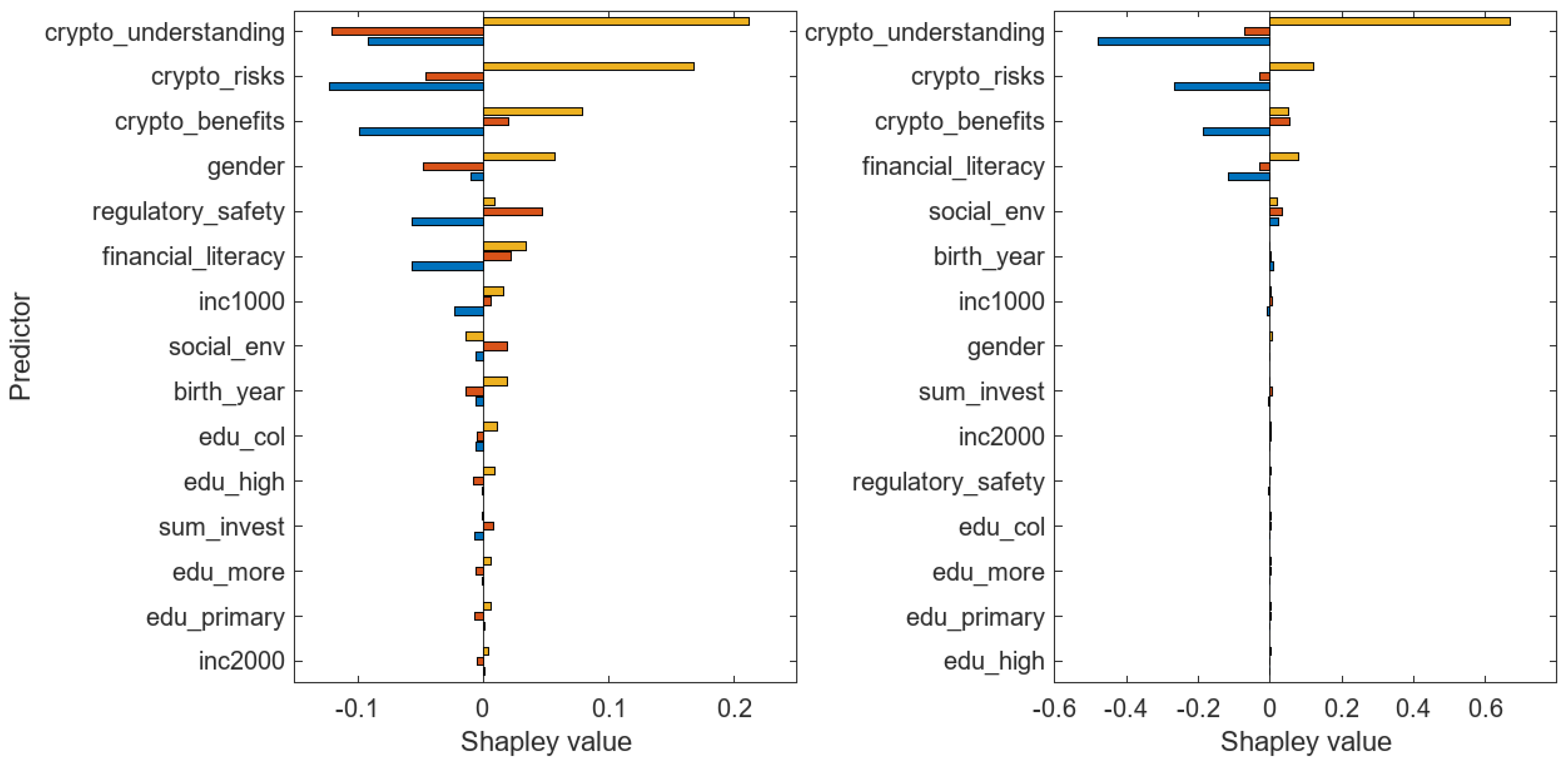
crypto_understanding	19	−0.0914	−0.1204	0.2117	−0.4788	−0.0701	0.6687
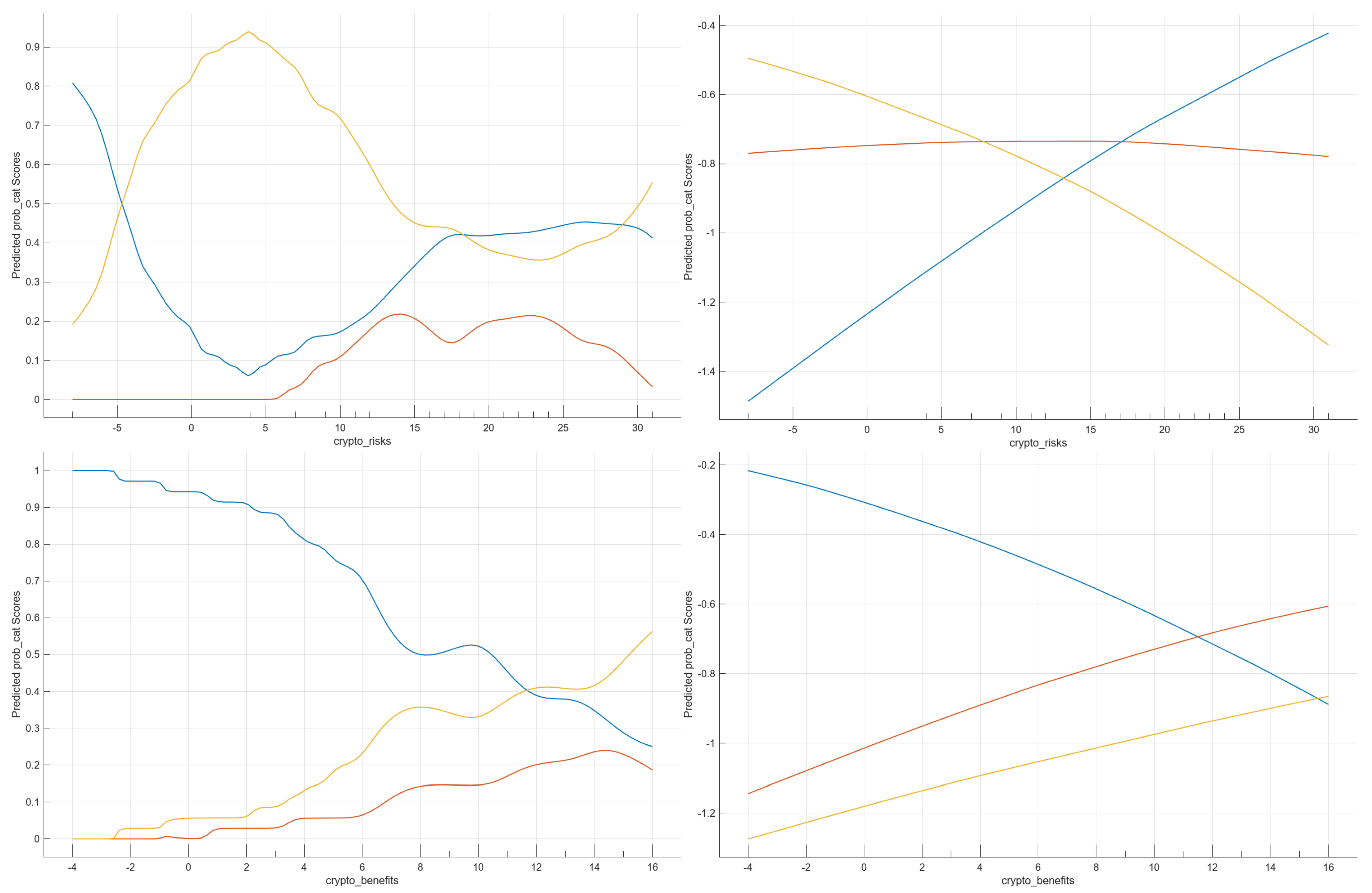
crypto_risks	12	−0.1223	−0.0454	0.1677	−0.4788	−0.0701	0.6687
crypto_benefits	15	−0.0987	0.0198	0.0789	−0.1876	0.0550	0.0494
gender	1	−0.0096	−0.0479	0.0574	−0.0012	−0.0030	0.0059
financial_literacy	15	−0.0563	0.0221	0.0342	−0.1178	−0.0293	0.0795
birth_year	1999	−0.0054	−0.0137	0.0191	0.0105	0.0035	−0.0029
inc1000	1	−0.0226	0.0063	0.0163	−0.0069	0.0069	0.0014
social_env	10	−0.0055	0.0193	−0.0139	0.0241	0.0338	0.0184
edu_col	1	−0.0060	−0.0050	0.0110	−0.0027	0.0009	0.0033
regulatory_safety	10	−0.0568	0.0473	0.0095	−0.0036	−0.0002	0.0035
edu_high	0	−0.0010	−0.0079	0.0089	−0.0006	0.0004	0.0029
edu_more	0	−0.0010	−0.0056	0.0066	−0.0020	0.0021	0.0024
edu_primary	0	0.0007	−0.0064	0.0057	−0.0012	0.0017	0.0023
inc2000	0	0.0006	−0.0046	0.0039	−0.0024	0.0030	0.0021
sum_invest	0	−0.0070	0.0081	−0.0011	−0.0040	0.0050	0.0003

Comment: prob_cat = likelihood of investing in crypto assets in the future; sum_invest = number of different investments; financial_literacy = perception of financial literacy; social_env = attitude of the social environment towards the crypto market; crypto_benefits = perceived benefits of crypto assets; crypto_risks = perceived risks of crypto assets; crypto_understanding = perceived understanding of crypto assets; regulatory_safety = perception of regulatory safety; edu_primary = highest educational level is primary school; edu_high = highest educational level is high school; edu_col = highest educational level is college; edu_more = highest educational level is bachelor’s, master’s, or PhD; inc1000 = monthly income is less than EUR 1000; inc2000 = monthly income is more than EUR 2000; birth_year = year of birth.

) involving a specific individual investor. We will additionally present and analyze how each attribute influenced the model’s prediction and decision, highlighting the most impactful factors that drove the outcome.

For this concrete test case (Table 5), we will present the visualization of Shapley values in Figure 1 for better understanding. As already mentioned, SHAP allows us to explain why this prediction was made by assigning Shapley values to each feature, showing how individual attributes contributed to the model’s decision in this case.

The visualization of SHAP values clearly illustrates how the method assigns importance to each explanatory variable, explaining their contribution to the final estimate. This can be interpreted similarly to regression coefficients, where higher absolute values indicate a greater impact on the prediction. Through this approach, we can observe how different variables influence the likelihood of investing in crypto assets across different classes.

A strong contrast is observed between class 1 (low likelihood of investment) and class 3 (high likelihood of investment). Specifically, if a variable has a positive impact on class 3, it has a negative impact on class 1, and vice versa. This suggests that the same predictors drive individuals either towards high or low investment likelihood, depending on their values. On the other hand, the impact on class 2 (moderate likelihood) is mixed—some variables exhibit the same influence as in class 1, while others align with class 3. This reflects the nature of the middle category, which represents individuals with uncertain or situational investment intentions, making it more difficult to establish clear predictor patterns.

A notable difference between the two models is in how predictor importance is distributed. In Kernel Naïve Bayes, the influence of variables is more evenly spread, meaning multiple predictors contribute similarly to the decision-making process. On the contrary, in Efficient Linear SVM, the first five variables have a significantly stronger impact, while the remaining variables play a more minor role. This indicates that the linear model places greater emphasis on a small set of key predictors, whereas the probabilistic model considers a broader set of influences.

Despite these differences, both models consistently identify the perceived understanding of crypto assets, perceived risks of crypto assets, and perceived benefits of crypto assets as the top three most important variables, ranked in the same order. In both models, these three predictors have a positive influence on class 3, meaning that individuals with higher knowledge, perceived risks, and perceived benefits of crypto assets are more likely to invest. Simultaneously, they have a negative influence on class 1, indicating that lower understanding and perceived benefits are associated with a low likelihood of investment. For class 2, the effects are more nuanced—crypto understanding and crypto risks have a negative impact, while crypto benefits has a positive impact. This suggests that moderate investors are more influenced by the perceived advantages of crypto assets rather than their risks or understanding level.

In terms of additional influential variables, Kernel Naïve Bayes assigns visible importance to three other constructs: perception of regulatory safety, perception of financial literacy, and attitude of the social environment towards the crypto market. In contrast, in Efficient Linear SVM, for variables financial_literacy and social_env remain impactful, but regulatory_safety does not play a significant role. This suggests that in the linear model, perceived regulatory aspects have a weaker direct influence on investment decisions compared to other social and financial factors.

Lastly, in both models, educational level does not appear to be a major determinant, as it falls into the lower end of the importance scale. This indicates that while education may play a role in financial decision-making more broadly, it is not a primary driver in predicting crypto investment likelihood compared to domain-specific knowledge and perceptions.

To sum up, the SHAP values visualization shows how each variable impacts the likelihood of investing in crypto, with clear differences between class 1 (low likelihood) and class 3 (high likelihood). Variables have opposing effects on these classes, while class 2 (moderate likelihood) shows mixed impacts. Kernel Naïve Bayes considers a broader set of predictors, while Efficient Linear SVM focuses more on a few key variables. Both models identify understanding, risks, and benefits of crypto assets as the most important predictors, with a stronger influence on class 3. Perception of regulatory safety plays a larger role in Kernel Naïve Bayes, while education is less important in both models.

After analyzing SHAP values to understand the local impact of individual features on predictions, we now shift our focus to a global explanation method—Partial Dependence (PD) [25]. While SHAP provides insight into how variables influence specific predictions, PD helps us examine the overall relationship between a feature and the model’s output across the entire dataset.

Partial Dependence is a widely used global interpretability technique that allows us to visualize how changes in a given predictor affect the model’s predictions while holding all other variables constant. This method estimates the marginal effect of a feature on the target variable by averaging out the influence of all other variables. Unlike local explanation techniques, PD helps uncover general trends rather than individual instance-level effects, making it particularly useful for detecting nonlinear relationships and threshold effects in machine learning models [26,27].

In the context of our study, PD will allow us to explore how key predictors, such as crypto understanding, perceived risks, and perceived benefits, influence the probability of an individual falling into each investment likelihood class (Figure 2). This will further validate our findings from SHAP analysis and provide additional insights into how our models make decisions.

Before we dive into the PD analysis, it is important to highlight that the asymmetry in the tornado charts and the nonlinear curves in the response functions for PD indicate a strong presence of nonlinearity. This further supports the justification for testing a wide range of machine learning methods, as they are better suited to capture such complex patterns.

Examining the behavior of different class curves, we see that the blue curve (class 1) and orange curve (class 3) always start at different levels and move in a mirrored fashion—if one increases, the other decreases, and vice versa. The red curve (class 2) exhibits a more variable pattern, sometimes behaving similarly to class 1 and other times aligning more with class 3. This reflects the uncertainty and transitional nature of class 2, reinforcing our previous findings that predicting this group is more difficult. This suggests that class 2 individuals share characteristics with both extreme groups, depending on the feature values.

Additionally, we observe a general trend of increasing likelihood for class 3 and decreasing for class 1 across all features, except for crypto_risks in Efficient Linear SVM. In most cases, the orange curve (class 3) ends at a higher value than it started, indicating that an increase in the given predictor leads to a higher probability of an individual being classified in class 3. Similarly, the blue curve (class 1) ends at a lower value, signifying a reduced likelihood of being in the lowest investment category. This trend aligns with our previous findings, as greater crypto understanding and perceived benefits positively correlate with higher investment interest. The exception for crypto_risks in Efficient Linear SVM suggests that for this model, risk perception does not follow the same straightforward pattern as other key predictors.

A key difference between the two models is the smoothness of the curves. The PD plots for Efficient Linear SVM (right) exhibit much smoother trends, whereas Kernel Naïve Bayes (left) shows more fluctuations and irregularities. This difference arises due to the nature of each model. Kernel Naïve Bayes operates on probability distributions, making its decision boundaries more sensitive to variations in the data, leading to less smooth curves. In contrast, Efficient Linear SVM learns a linear separation between classes, resulting in more stable and consistent relationships between predictors and outcomes.

Based on this finding, we determine that the optimal model, despite initially considering both as optimal, is the Efficient Linear SVM. This choice is logical because the smoother trends in its PD plots indicate more stable and consistent relationships between predictors and outcomes, reducing sensitivity to variations in the data. Such stability enhances interpretability and reliability, making it a preferable option. Notably, this smoothness is observed across all numerical variables, with the remaining PD plots presented in the Appendix A (Figure A1, Figure A2 and Figure A3).

Beyond the methodological comparison, the practical implications of our findings highlight actionable insights for investment firms and financial institutions. By identifying key factors that predict crypto market participation, firms can tailor their engagement strategies to attract potential investors more effectively. For instance, predictive modeling can be integrated into client segmentation strategies, enabling firms to personalize financial products and advisory services based on an individual’s likelihood to invest. Additionally, risk assessment frameworks can be refined using these insights to better evaluate market trends and investor behavior. Future applications of this research could also include real-time decision-making tools that dynamically adapt to evolving investor sentiment, further enhancing firms’ ability to navigate the rapidly changing crypto landscape.

Our study adds significant value by bridging the gap in previous research, which primarily focused on traditional investment theories such as the Theory of Planned Behavior (TPB), Behavioral Finance, and the Technology Acceptance Model (TAM). By integrating these classical theories with advanced artificial intelligence methods, our research provides more accurate predictions of investment decisions. This hybrid approach not only enhances the understanding of investor behavior but also has direct practical implications for financial institutions and policymakers in improving strategies for engaging investors in the crypto market.

Moreover, while our study offers valuable insights, a larger and more diverse dataset could enhance the generalizability of our findings. Future research should employ broader sampling methods to better capture different investor profiles and minimize potential biases. Additionally, conducting a longitudinal study would allow for an analysis of how investment intentions evolve over time in response to market fluctuations, regulatory changes, and broader economic conditions, providing a more comprehensive understanding of investor behavior.

5. Conclusions

5.1. Key Findings

Our study aimed to explore the demographic, behavioral, and financial factors influencing investment decisions in crypto assets and to identify the most effective machine learning models for predicting crypto asset investors. Our analysis revealed that the Efficient Linear SVM and Kernel Naïve Bayes models were the most optimal for this task. Contrary to the common belief that tree-based or deep learning models offer the best results, we found that simpler models, with appropriate feature representation and well-calibrated decision boundaries, could perform just as effectively. Furthermore, the use of Explainable AI (XAI) methods, specifically SHAP and Partial Dependence Plots, highlighted the most influential factors, such as crypto understanding, perceived risks, and perceived benefits, and showed how their effects varied across investor classes.

These findings are significant in both theoretical and practical contexts. By integrating classical investment theories—such as the Theory of Planned Behavior (TPB), Behavioral Finance, and the Technology Acceptance Model (TAM)—with advanced machine learning techniques, our research offers a novel contribution to the literature. We bridge traditional models with modern AI methods, providing a more accurate and dynamic understanding of investor behavior, particularly in the emerging crypto asset market. Our results suggest that demographic, behavioral, and psychological factors are crucial in predicting investment decisions and that these factors interact in complex ways that simpler machine learning models can effectively capture.

5.2. Implications

Our research enhances the theoretical understanding of investor behavior by combining well-established investment theories with advanced AI techniques. This hybrid approach offers more precise insights into how demographic, behavioral, and psychological factors influence investment decisions in the crypto market. By extending classical models such as TPB, Behavioral Finance, and TAM to include machine learning, our study provides a more comprehensive framework for predicting investor behavior, particularly in emerging markets like crypto. The findings highlight the importance of these theories in understanding the complexity of investor decision-making and provide a foundation for future research to build upon.

From a practical standpoint, our findings suggest that investment firms can leverage these insights to better understand and target different segments of crypto investors. By tailoring marketing campaigns and financial products to meet the specific needs of both traditional and crypto investors, firms can more effectively engage potential investors. Additionally, our results underscore the importance of educational initiatives focused on financial literacy and crypto asset knowledge, which could help build investor trust and confidence. Regulators can also use the investor profiles identified in this study to target individuals with a higher likelihood of investing, raising awareness about the risks associated with crypto-assets. Moreover, AI methods can be employed to better manage price risks and provide more proactive strategies to enhance investor protection and market stability.

5.3. Future Research and Limitations

Despite the valuable contributions of our study, there are several limitations. The reliance on convenience sampling through social media and personal networks may have introduced selection bias, limiting the representativeness of the sample. The relatively small dataset also restricted the complexity of models we could test, potentially affecting the generalizability of our findings. Additionally, self-reported data may have introduced response bias, especially in subjective assessments of financial literacy and risk perception.

Future research should aim to expand the dataset with a more diverse and representative sample, capturing a broader range of investor profiles. Incorporating additional behavioral and psychological factors would further enhance the analysis and provide a deeper understanding of investor motivations. Furthermore, since our study was cross-sectional, replicating this research in the future would offer valuable insights into the dynamic nature of investor behavior over time. This would allow for a better understanding of how market fluctuations, regulatory changes, and economic conditions influence investment intentions in the volatile crypto market.

References

- Nakamoto, S. Bitcoin: A Peer-to-Peer Electronic Cash System. 2009. Available online: https://bitcoin.org/bitcoin.pdf (accessed on 8 January 2025).
- Seoyouung, K.; Atulya, S.; Daljeet, V. Crypto-Assets Unencrypted. J. Invest. Manag. Forthcom. 2018, p. abs/3117859. Available online: https://ssrn.com/abstract=3117859 (accessed on 8 January 2025).
- Koehler, S.; Dhameliya, N.; Patel, B.; Anumandla, S.K.R. AI-Enhanced Cryptocurrency Trading Algorithm for Optimal Investment Strategies. Asian Account. Audit. Adv. 2018, 9, 101–114. [Google Scholar]
- Leahy, E. AI-Powered Bitcoin Trading: Developing an Investment Strategy with Artificial Intelligence; John Wiley & Sons: Hoboken, NJ, USA, 2024. [Google Scholar]
- Babaei, G.; Giudici, P.; Raffinetti, E. Explainable artificial intelligence for crypto asset allocation. Financ. Res. Lett. 2022, 47, 102941. [Google Scholar] [CrossRef]
- Kahneman, D.; Tversky, A. Prospect Theory: An Analysis of Decision under Risk. In Handbook of the Fundamentals of Financial Decision Making; World Scientific Handbook in Financial Economics Series; World Scientific: Singapore, 2013; pp. 99–127. [Google Scholar]
- Ajzen, I. The theory of planned behavior. Organ. Behav. Hum. Decis. Process. 1991, 50, 179–211. [Google Scholar] [CrossRef]
- Pilatin, A.; Dilek, Ö. Investor intention, investor behavior and crypto assets in the framework of decomposed theory of planned behavior. Curr. Psychol. 2024, 43, 1309–1324. [Google Scholar] [CrossRef]
- Mittal, S.K. Behavior biases and investment decision: Theoretical and research framework. Qual. Res. Financ. Mark. 2022, 14, 213–228. [Google Scholar] [CrossRef]
- Davis, F.D. Perceived usefulness, perceived ease of use, and user acceptance of information technology. MIS Q. Manag. Inf. Syst. 1989, 13, 319–339. [Google Scholar] [CrossRef]
- Almeida, J.; Gonçalves, T.C. A systematic literature review of investor behavior in the cryptocurrency markets. J. Behav. Exp. Financ. 2023, 37, 100785. [Google Scholar] [CrossRef]
- Ante, L.; Fiedler, I.; Von Meduna, M.; Steinmetz, F. Individual Cryptocurrency Investors: Evidence from a Population Survey. Int. J. Innov. Technol. Manag. 2022, 19, 2250008. [Google Scholar] [CrossRef]
- Colombo, J.A.; Yarovaya, L. Are crypto and non-crypto investors alike? Evidence from a comprehensive survey in Brazil. Technol. Soc. 2024, 76, 102468. [Google Scholar] [CrossRef]
- Jin, S.V. “Technopian but lonely investors?”: Comparison between investors and non-investors of blockchain technologies, cryptocurrencies, and non-fungible tokens (NFTs) in Artificial Intelligence-Driven FinTech and decentralized finance (DeFi). Telemat. Inform. Rep. 2024, 14, 100128. [Google Scholar] [CrossRef]
- Tzavaras, C. Investor Demographics and their Impact on the Intention to Invest in Cryptocurrencies: An Empirical Analysis of Crypto Investors and Non-Crypto Investors. Utrecht University. 2023. Available online: https://studenttheses.uu.nl/bitstream/handle/20.500.12932/45007/Tzavaras%2CC._5437393.pdf?sequence=1&isAllowed=y (accessed on 24 March 2025).
- Caelen, O. A Bayesian interpretation of the confusion matrix. Ann. Math. Artif. Intell. 2017, 81, 429–450. [Google Scholar] [CrossRef]
- Muschelli, J. ROC and AUC with a Binary Predictor: A Potentially Misleading Metric. J. Classif. 2020, 37, 696–708. [Google Scholar] [CrossRef] [PubMed]
- Webb, G.I. Naïve Bayes. In Encyclopedia of Machine Learning and Data Mining; Springer: Berlin/Heidelberg, Germany, 2017; Available online: https://www.researchgate.net/profile/Geoffrey-Webb/publication/306313918_Naive_Bayes/links/5cab15724585157bd32a75b6/Naive-Bayes.pdf (accessed on 24 March 2025).
- Pérez, A.; Larrañaga, P.; Inza, I. Bayesian classifiers based on kernel density estimation: Flexible classifiers. Int. J. Approx. Reason. 2009, 50, 341–362. [Google Scholar] [CrossRef]
- John, G.H.; Langley, P. Estimating Continuous Distributions in Bayesian Classifiers. In Proceedings of the Eleventh Conference on Uncertainty in Artificial Intelligence, Bellevue, WA, USA, 11–15 July 2013; pp. 338–345. [Google Scholar]
- Suthaharan, S. Support Vector Machine. In Machine Learning Models and Algorithms for Big Data Classification; Springer: Boston, MA, USA, 2016; pp. 207–235. [Google Scholar]
- Wu, J.; Yang, H. Linear Regression-Based Efficient SVM Learning for Large-Scale Classification. IEEE Trans. Neural Netw. Learn. Syst. 2015, 26, 2357–2369. [Google Scholar] [CrossRef] [PubMed]
- Angelov, P.P.; Soares, E.A.; Jiang, R.; Arnold, N.I.; Atkinson, P.M. Explainable artificial intelligence: An analytical review. Wiley Interdiscip. Rev. Data Min. Knowl. Discov. 2021, 11. [Google Scholar] [CrossRef]
- Mane, D.; Magar, A.; Khode, O.; Koli, S.; Bhat, K.; Korade, P. Unlocking Machine Learning Model Decisions: A Comparative Analysis of LIME and SHAP for Enhanced Interpretability. J. Electr. Syst. 2024, 20, 598–613. [Google Scholar] [CrossRef]
- Parr, T.; Wilson, J.D. Partial dependence through stratification. Mach. Learn. Appl. 2021, 6, 100146. [Google Scholar] [CrossRef]
- Greenwell, B.M. pdp: An R Package for Constructing Partial Dependence Plots. R J. 2017, 9, 421–436. [Google Scholar]
- Friedman, J.H. Greedy function approximation: A gradient boosting machine. Ann. Stat. 2001, 29, 1189–1232. [Google Scholar] [CrossRef]