Abstract
Introduction: Ensuring vehicular cybersecurity is a critical challenge due to the increasing connectivity of modern vehicles, and traditional centralised learning approaches for intrusion detection pose significant privacy risks, as they require sensitive data to be shared from multiple vehicles to a central server. Objective: The aim of this study is therefore to develop an in-vehicle intrusion detection system (IVIDS) that integrates federated learning (FL) with neural networks, enabling decentralised and privacy-preserving detection of cyberattacks in vehicular networks. The proposed system extends previous research by detecting a broader range of attacks (eight types) and exploring different deep learning architectures. Methods: This study employs an extended version of the publicly available VeReMi dataset to train and evaluate multiple neural network architectures, including Multilayer Perceptrons (MLPs), Gated Recurrent Units (GRUs), and Long Short-Term Memory (LSTM) networks. Federated learning is utilised to enable collaborative model training across multiple vehicles without sharing raw data. Various data preprocessing techniques and differential privacy mechanisms are also explored. Results and Conclusions: The experimental results demonstrate that LSTM networks outperform both MLP and GRU architectures in classifying vehicular cyberattacks. The best LSTM model, trained with two previous message lags and standard normalisation, achieved a classification accuracy of 96.75% in detecting eight types of attacks, surpassing previous studies, and demonstrating the potential of applying neural networks designed to work with time series data.
1. Introduction
We live in a society where automation is commonplace. In 2022, it was estimated that there were about 30 billion active IoT (Internet of Things) devices worldwide [1], while in 2024, the number was estimated at 43 billion. Of these, it was calculated that specifically 15.14 billion were connected IoT devices, a figure expected to double by 2030 [2], as the IoT market is experiencing rapid growth, with IoT connections increasing at an average rate of 20% per year [3].
We have a significant presence of sensors and connected devices in all areas. In medicine, sensors are used for the constant monitoring of patients in hospitals and clinics, allowing real-time tracking of parameters such as heart rate, blood pressure, and glucose levels, therefore improving emergency response capabilities and facilitating early diagnosis [4,5,6]. Furthermore, the integration of IoT devices in the medical field enables the telemonitoring of patients in their homes, reducing costs, improving comfort, and promoting personalised care [7].
On the other hand, the industrial sector is where IoT devices are used the most [2]. One of the main applications is real-time monitoring, both of machinery and its interaction with people, as well as production processes, therefore facilitating the collection and analysis of data to optimise operational efficiency and predict potential failures, while also improving productivity [8,9,10].
Regarding agriculture, IoT sensorization has also extended to crops. Numerous studies employ probes equipped with sensors for the monitoring and prediction of various soil properties, such as moisture, temperature, and salinity [11,12,13,14], allowing for a more intelligent use of the available resources.
Another key field in IoT applications is the automotive sector. IoT devices have revolutionised this industry not only externally to the vehicle, by enabling real-time monitoring and communication between vehicles, infrastructure, and users, but also internally, through advanced sensorisation and connectivity, making it possible to track engine performance, optimise fuel consumption, and enhance safety features, such as collision avoidance and lane-keeping assistance. Moreover, IoT plays a pivotal role in the development of autonomous vehicles, facilitating the collection and analysis of vast amounts of data to ensure precise navigation and decision-making [15,16,17,18,19].
Taking all this context into account, it is of vital importance to ensure the secure use of IoT devices, particularly in sectors such as medicine or automotive, where a communication failure or, even worse, an attack or intrusion, could result in the loss of human lives. This is, precisely, where the importance of developing intrusion detection systems comes into play, aiming to prevent attackers from taking control of, for example, a vehicle and transmitting erroneous data on speed or position, thereby destabilising the entire communication system between vehicles and causing traffic accidents.
In recent years, numerous studies have been conducted to enhance the security of in-vehicle systems, particularly through the development of innovative intrusion detection systems (IVIDSs) for the Controller Area Network (CAN). For instance, [20,21,22] explored the application of machine learning algorithms in detecting anomalies within vehicular networks, demonstrating significant improvements in detection accuracy. Similarly, other studies [23,24] investigated the use of blockchain technology to enhance the integrity and security of communication between vehicles. Furthermore, Xun et al. in [25] proposed VehicleEIDS, a methodology that leverages external voltage signals for intrusion monitoring without impacting CAN bandwidth, achieving over 97% accuracy in detecting abnormal signals, and Tanaka et al. in [26] further advanced the field by combining density ratio estimation with neural networks to detect and interpret malicious packet injections, offering deeper insights into attack vectors.
Other studies have focused on improving detection accuracy while optimising resource usage [27,28]. For example, Zhang et al. in [29] developed Binarized Convolutional Neural Networks (BCNNs), which increased detection accuracy while significantly reducing memory and processing time, making them particularly advantageous for in-vehicle applications.
Although these studies have represented significant advancements in this research field, many, such as those presented in [30,31], exhibit certain limitations. Notably, all of them rely on training a global model based on different versions of the VeReMi dataset, which is specifically designed for intrusion detection in vehicular environments [32]. This approach introduces a severe potential privacy risk since, even though the dataset consists of simulated data, if real-world driving scenario data were to be used—collected from multiple vehicles—to train such a global model following the approach adopted in these studies, each vehicle would need to share and transmit its data to a centralised structure or server, where all data would be stored and the model would be hosted for training. Consequently, a potential attacker could extract these data either by compromising the server or by performing a man-in-the-middle attack, intercepting the network traffic and exfiltrating data during transmission.
To address this limitation, this study proposes the development of an in-vehicle intrusion detection system (IVIDS) that combines artificial intelligence techniques with a distributed and scalable approach, namely federated learning, following a similar approach to that of [33], allowing multiple vehicles to collaboratively learn from data without sharing sensitive information. The proposed system is designed to operate in an environment involving multiple vehicles communicating with each other and with road infrastructure. Furthermore, this study extends the number of detected attacks from five, as in [33], to eight attacks, therefore allowing for a broader detection capability, increasing the robustness of the proposed intrusion detection system against a wider variety of threats. To achieve this, we utilise an extended version of the publicly available VeReMi dataset hosted on Kaggle, whose description is provided in [30]. Moreover, while in [33] only Multilayer Perceptrons (MLPs) were analysed, in this research we have also experimented with other types of architectures and networks, specifically Long Short-Term Memory (LSTM) networks and Gated Recurrent Units (GRUs). This is because the VeReMi data consists of messages exchanged between vehicles, which fundamentally constitutes a time series. In addition, another novelty presented in this study is the examination of the impact of differential privacy, which is a technique that adds noise to the model parameters to ensure that individual data points cannot be distinguished, on model performance.
Therefore, the following are the main innovations and contributions introduced by this paper:
- -
- Implementation of federated learning, allowing multiple vehicles to collaborate in model training without sharing sensitive data, which mitigates the risks associated with data centralisation.
- -
- Extension of the detection system, increasing the number of identifiable attacks from five (as in [33]) to eight, which significantly enhances the robustness and scope of protection.
- -
- Comparative evaluation between different types of architectures, including Multilayer Perceptrons (MLPs), Long Short-Term Memory (LSTM) networks, and Gated Recurrent Units (GRUs), leveraging the time series nature of vehicular communication data.
- -
- Study of the effect of implementing differential privacy techniques with different types of noise (Gaussian and Laplacian) on the performance and accuracy of the model.
Finally, although it will be discussed in much more detail throughout the paper, it is worth noting that among the primary findings of this study, the superiority of LSTM networks over the other two architectures, MLP and GRU, stands out, achieving an accuracy of 96.75%, surpassing the other models. Furthermore, the negative impact of differential privacy, both for Gaussian and Laplacian noise, on the model’s accuracy is also highlighted, with accuracy dropping from 96.75% to 20.62%.
In this section, the motivation for this study has been presented, along with an analysis of the main related works. The remainder of the paper is structured as follows: Section 2 describes the methodology adopted, detailing the federated learning approach, the data preprocessing steps, and the chosen models; Section 3 presents the main results of the study; and Section 4 outlines the conclusions drawn from this research.
2. Materials and Methods
2.1. Federated Learning Approach
Figure 1 depicts a diagram that shows, in a simple way, a centralised learning process, in which several vehicles send their data to a central server (hosted, for example, in road infrastructure), where all the data are stored. Once all the data from all the vehicles are collected, they are divided into train and test sets, and the learning process begins, in which a global model, for example, a neural network, iterates a certain number of epochs over the training set. Then, once the model completes its learning, it is evaluated on the test set.
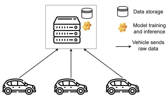
Figure 1.
Centralised learning architecture: all data are collected and processed on a central server.
However, this centralised approach entails significant privacy risks. Firstly, since all data are sent and stored on a central server, there is significant exposure to security attacks that could compromise the sensitive information of the vehicles. If a malicious actor gains access to the central database, they would have access to the complete data of all participants, which represents a greater risk compared to distributed architectures.
Moreover, the constant sending of data from the vehicles to the central server introduces additional vulnerabilities in transmission. If the communication is not adequately encrypted, an attacker could intercept the data during their transfer, extracting critical information about driving habits, location, and vehicle behaviour. Even if robust encryption is implemented, the mass collection of data at a single point creates an attractive target for directed attacks.
On the other hand, the centralisation of data can also generate issues of digital sovereignty, especially when the data from vehicles located in different regions are stored on servers that may be subject to foreign regulations, where there may be laws that do not necessarily protect the privacy of drivers, and where the entity managing the central server may use the vehicular data (which often contain sensitive information) to monitor driver behaviour or even for commercial purposes without the explicit consent of the users.
To address these potential privacy issues, Figure 2 proposes a federated learning scenario, where clients no longer need to share their data with a central server where everything is stored. With this distributed approach, a global model is randomly initialised on the central server, and its initial weights are sent to the vehicles (clients) that connect to the road infrastructure where the server is hosted. In this way, each vehicle has its own local version of the model, and using its own data, for example from vehicle-to-vehicle (V2V) communications, without needing to send and store them on an external server, they train their local version of the model for a few epochs. Then, they send back to the server only the weights of the local models, which are aggregated by the server following some strategy and sent back to the clients in the next round of federated learning. Again, the clients will locally train the new version of the model for a few epochs and send the local weights to the server, which will aggregate them again, and so on for a certain number of training rounds. Furthermore, at the end of each round, the server can ask the clients to evaluate the aggregated global model on their own data, as well as perform a global evaluation with test data that the server itself contains and that are independent of the clients’ data.
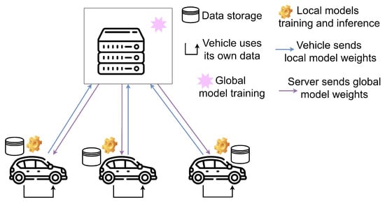
Figure 2.
Federated learning architecture: data are kept locally on each device, while the model is trained collaboratively through parameter aggregation, preserving data privacy.
In this way, the federated learning approach not only improves privacy preservation by avoiding the transmission of sensitive data, but also allows for a more representative evaluation of the model. By keeping the data on each vehicle, the risk of exposure to attacks and unauthorised access is minimised, ensuring that the personal information of the drivers is neither stored nor processed centrally.
Moreover, this strategy allows the model to learn more equitably from the diversity of data distributed among the vehicles. In a centralised environment, the model may be biased by the distribution of data available on the server, whereas with federated learning, each client trains locally on its own data, ensuring that the global model better captures the inherent variability of different driving scenarios.
Another significant advantage, as already mentioned, is the improvement in model evaluation, since at the end of each training round, the clients can evaluate the global model with their own real data, providing more representative metrics of performance under real usage conditions.
Furthermore, an “extra layer” of security can be added to the distributed approach of federated learning to further enhance privacy: differential privacy. This technique introduces random noise into the data or model gradients before they are sent to the server, making it difficult to identify sensitive information even if the processed data were intercepted. Its main benefit is that it provides mathematical guarantees of privacy, reducing the risk of data leaks. However, this increased privacy comes at a cost in terms of performance, as the introduced perturbation can impact the model’s convergence and degrade its accuracy, especially if the level of added noise is high.
2.2. Data Preprocessing
The data used in this study were obtained from Kaggle (https://www.kaggle.com/datasets/cyberdeeplearning/VeReMi-extension-clean-data (accessed on 3 April 2025)). As stated in Section 1, the dataset constitutes an extension of the publicly available VeReMi dataset. However, it is worth noting that, although the dataset contains 18 different classes (normal behaviour and 17 types of attacks), this study is focused exclusively on the detection of attacks related to position and speed spoofing (referred to as faults, which constitute 8 of the 17 types of attacks included in the dataset used), as these types of attacks have a critical and direct impact on the safety and proper operation of vehicular networks. Particularly, the faults studied are described in Table 1:

Table 1.
Descriptions and main impacts of the eight attack types studied.
The dataset initially consisted of 30 columns:
- -
- Type: type of message (e.g., GPS, BSM).
- -
- SendTime: time the message was sent.
- -
- Sender: identifier of the message sender.
- -
- SenderPseudo: pseudonym of the sender.
- -
- MessageID: unique identifier of the message.
- -
- Class: number indicating the class of the message (e.g., normal, constant offset position, etc).
- -
- Posx, posy, posz: X, Y, and Z coordinates of the vehicle’s position.
- -
- , , : noise associated with the X, Y, and Z coordinates of the vehicle’s position.
- -
- Spdx, spdy, spdz: speed in the X, Y, and Z axis.
- -
- , , : noise associated with the speed in the X, Y, and Z axes.
- -
- Aclx, acly, aclz: acceleration in the X, Y, and Z axes.
- -
- , , : noise associated with the acceleration in the X, Y, and Z axes.
- -
- Hedx, hedy, hedz: heading direction in the X, Y, and Z axes.
- -
- , , : noise associated with the heading direction in the X axis.
Regarding this dataset, a study of the data was conducted, and feature selection was performed to extract only those columns relevant for future models to differentiate each type of attack. First of all, all columns measuring variables related to the Z axis were removed, because in all of them, the examples had a value of 0.0, which does not provide any information. For this same reason, the column type was also removed, as it always has the same value in all examples. Moreover, while [30] retains the pseudoID variable, in this case, all variables related to identifiers were removed for two reasons:
- -
- When putting the model into production on data from different vehicles, the ID numbering sequences do not necessarily match those used for training, which could cause serious generalisation issues.
- -
- In the dataset, the messages sent by a vehicle correspond only to one type of attack, so all messages with the same senderID (or pseudoID) also correspond only to one type of attack, as the values of these columns are unique for each vehicle. Therefore, if these variables are not removed, the model could “memorise” which IDs correspond to each type of attack in the dataset, again causing serious generalisation issues.
Furthermore, the columns related to acceleration and heading were removed; as indicated in [30], all simulated attacks in the original VeReMi dataset are related to position and speed. This is also demonstrated by Figure 3, which shows a correlation matrix where it is clearly observable that the correlation between these columns and the attacks is 0.00. For this same reason, the noise variables in the positions and speed on the different axes were also removed.
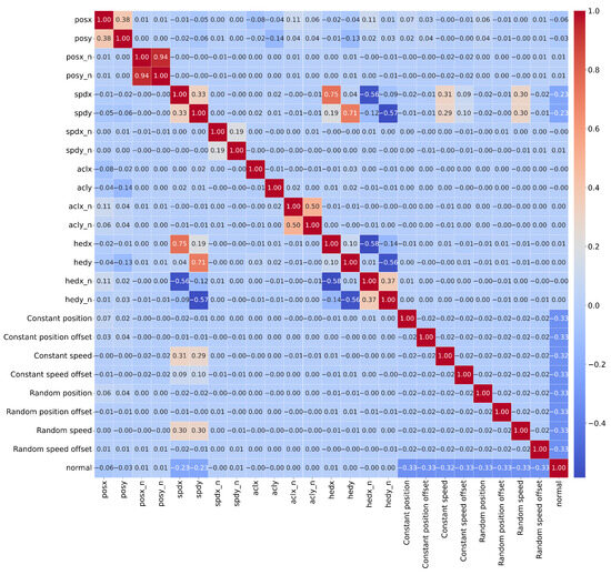
Figure 3.
Correlation matrix between numerical attributes and attack types.
Once the feature selection was completed, the presence of imbalance in the dataset was studied, obtaining the results shown in Table 2, where a clear imbalance can be observed between the normal behaviour and the rest of the 8 studied attacks, each with around 42,000 examples.
Table 2.
Original number of examples for each attack type.
To address the significant imbalance between normal behaviour and the various attack classes present in the VeReMi dataset, we opted to perform undersampling, using Random Under-Sampling (RUS), of the majority class instead of applying oversampling to the minority classes as conducted in [33]. This decision is based on the fact that oversampling, through synthetic sample generation techniques, can increase the risk of overfitting by replicating or creating artificial examples that do not provide new information, overlap with other examples, and even introduce noise into the model. In contrast, undersampling allows for balancing the class distribution by controlled reduction in the number of normal behaviour examples, facilitating the model’s learning of relevant patterns from the attack classes without losing diversity in data representation. This approach not only optimises computational performance during training but also aligns with previous studies in the field of imbalanced dataset classification, which have demonstrated the effectiveness of reducing the majority class to preserve the representativeness of the minority classes [34].
On the other hand, considering that the dataset constitutes a time series, as it is composed of messages sent by different vehicles at different points in time, a time series-based approach was adopted, for which 3 types of datasets were created:
- -
- The first type, in addition to the variables that were not eliminated (positions and speeds on the X and Y axes), contains a new variable for each original variable with a lag of 1. That is, variables with the values of the previous message for each original variable were added.
- -
- The second type of dataset includes two new variables for each non-eliminated variable, corresponding to the values of the two previous messages (lags of 1 and 2).
- -
- The third type of dataset was constructed by adding five new variables for each variable, corresponding to the values of the five previous messages (lags of 1 to 5).
To perform this lag aggregation, the senderID variable was taken into account. Thus, for each message, only the messages sent by the same vehicle at a previous timestamp (same senderID and sendTime less than that of the current message) were considered as previous. Therefore, as the number of lags considered increases, the amount of historical information available for each message, and consequently, the dimensionality, also increases.
The next notable phase of the preprocessing carried out on the data was normalisation. To choose the most suitable normalisation methods for the dataset, the distribution of the attributes was studied, as shown in Figure 4.
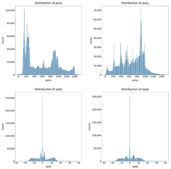
Figure 4.
Distribution of the position and speed attributes on the X and Y axes.
Moreover, the Shapiro–Wilk and Kolmogorov–Smirnov (KS) numerical methods were used to study the approximation of the different attributes to the theoretical uniform and normal distributions. The results of these tests are presented in Table 3, where, although it is concluded that the data do not fit a normal distribution according to the Shapiro–Wilk test (p-value ≈ 0 in all cases), the KS test values show that in all variables (especially in posy, spdx, and spdy) the distribution approximates more closely to the normal than to the uniform (for example, KS Normal of 0.0909 in posy versus KS Uniform of 0.2613), suggesting that, although perfect normality is not met, the data structure is closer to a Gaussian distribution than to a uniform distribution. Taking this into account, the normalisation methods Min–Max scaler, Standard scaler, and Robust scaler were studied.
Table 3.
Detailed results of the Shapiro–Wilk test and Kolmogorov–Smirnov (KS) test for uniform and normal distributions for each variable.
Min–Max scales each variable in the range [0, 1] by applying the linear transformation [35] described in Equation (1).
In this way, it can be ensured that the original shape of the data distribution is preserved [36]. However, it is an extremely sensitive technique to outliers [37], which is common in sensor data and measurements of positions and speed, as demonstrated in Figure 5, where a very strong presence of outliers in the speed variables is observed. Therefore, the application of Min–Max could lead to the compression of most of the information about speed into a very narrow range, as it would consider the two most extreme outliers as the minimum and maximum.

Figure 5.
Boxplots for analysing the presence of outliers in speed and position attributes.
On the other hand, standard normalisation transforms the data to have a mean of zero and a standard deviation of one [35], following Equation (2). It assumes that the data are normally distributed [37].
This technique often facilitates the convergence of certain algorithms and optimisation methods, such as neural networks, which are the type of models that will be used in this study. Moreover, since the KS tests showed a certain closeness to the normal distribution and the speed variables are centred around 0, it is considered an appropriate option.
On the other hand, robust normalisation scales the data using the median and the interquartile range (IQR):
Furthermore, it is less sensitive to extreme values, precisely because it uses the median and the IQR [35,37], which are robust statistics. It also maintains the relative shape of the distribution without allowing outliers to dominate the scaling.
To enable training based on federated learning, a global test set (for each type of the previous datasets) of about 900 examples was reserved first. To make the division, all messages from 5 randomly chosen senderIDs were selected for each type of attack (in addition to normal behaviour). By completely selecting all messages from the same vehicle, it is ensured that there is no data leakage between training and testing, thus allowing its generalisation capability on unseen data to be truly measured. Moreover, to compare the performance of different techniques and models, it is necessary to have a constant test set to make a fair and consistent comparison.
After saving these global test sets, the remaining part of each dataset was divided into different parts, simulating that each part corresponded to the local data of a client. Again, to make these partitions, the senderID column was taken into account, so that for each studied class (the 8 faults and normal behaviour), 50 vehicles were randomly selected. It is worth noting that two or more partitions may contain some repeated vehicles. However, this reflects reality, where during V2V communication, a vehicle sends its messages to different vehicles in the network, so several vehicles will have messages from the same sender. All the partitions created have between 46,000 and 52,000 examples each. For each type of dataset, 10 partitions were created.
2.3. Models
2.3.1. MLP
The MLP is a feedforward neural network composed of one or more hidden layers between the input and output, where each neuron applies an activation function (e.g., ReLU) to the linear combination of its inputs. Training is achieved through backpropagation to adjust the weights and minimise a cost function [38,39].
MLPs have been widely used in various intrusion detection scenarios [40,41,42], having demonstrated high accuracy in detecting network intrusions, with studies reporting average accuracies of up to 97% [43].
Nonetheless, although [33] have achieved high accuracies in detecting 5 types of attacks from the VeReMi dataset, an MLP processes each sample independently, thus not intrinsically exploiting the sequential dependency present in temporal data like VeReMi, where the examples are messages exchanged between vehicles over time. Therefore, in this study, we propose the use of other types of neural networks, specifically GRUs and LSTMs, which have a greater capacity to model patterns and trends over time, with the aim of leveraging the temporal dependencies inherent in the VeReMi data, and improving the accuracy of the predictions.
2.3.2. GRU
GRU is a variant of Recurrent Neural Networks (RNNs) that introduces gate mechanisms to control the flow of information. Specifically, it has an update gate and a reset gate that allow the model to decide when to incorporate new information and when to forget previous data [44].
GRUs offer distinct advantages over MLPs in intrusion detection systems, particularly in terms of accuracy and computational efficiency, since, as already stated, they are designed to handle sequential data effectively, making them well suited for analysing network traffic patterns, which are inherently temporal [45]. They have achieved up to 99% on specific datasets, such as the CSE-CIC-IDS2018 Dataset, UNSW-NB15, and BoT-IoT [46,47].
2.3.3. LSTM
Like GRUs, LSTM networks are also a variant of RNNs, but they are designed to overcome the vanishing gradient problem by incorporating a memory structure with cells and three types of gates: input, forget, and output. These gates allow the network to decide what information to retain, forget, or pass on to the next stage, facilitating the learning of long-term dependencies and the discrimination of subtle patterns in sequential data [48,49,50], which is crucial in critical applications such as network intrusion detection.
These types of networks have also been successfully applied in the field of intrusion detection. For example, in [51], a combination of Spark ML for anomaly detection and a Conv–LSTM network for misuse detection in the network was used, achieving an accuracy of 97.29%. On the other hand, in [52], three models based on LSTMs were implemented: LSTM without dimensionality reduction, LSTM with Principal Component Analysis (PCA), and LSTM with Mutual Information (MI); they were tested on the KDD99 dataset for binary and multi-class classification tasks. It was concluded that the LSTM-PCA model obtained the best results, especially with two components, achieving an accuracy of 99.44% in binary classification and 99.39% in multi-class classification.
The selection of these three types of models has been based on two main aspects: the diversity in the data modelling approach and the alignment with both the characteristics of FL and the characteristics of the VeReMi dataset.
On the one hand, the MLP model is expected to act as a reference model, chosen due to the simplicity of its structure and the effectiveness it has achieved in some cases, as explained. However, it is not a model specifically designed for scenarios with data dependencies, as in this case, where the VeReMi dataset consists of time-sequenced messages. Therefore, Recurrent Neural Network-based models, such as GRU and LSTM, seem much more suitable in this case, as both architectures, as indicated, are designed to process time series, allowing the extraction of patterns and relationships over time that are critical for detecting anomalous behaviours in vehicular communication flows.
On the other hand, in FL, the use of neural networks is ideal, as they are capable of being trained in a distributed manner and adapting to heterogeneous data coming from different nodes.
2.4. Differential Privacy
As explained earlier, differential privacy (DP) is a technique that adds noise to the output of a function to obscure individual contributions in the data. In this approach, DP is applied to the local weights of each client’s models before being sent to the server for aggregation, ensuring that the sensitive information of each device remains protected [53,54,55].
Particularly, two perturbation mechanisms will be evaluated: the Laplace and the Gaussian. The former is the most widely used due to its versatility, as it adapts well to almost any type of data; however, if too much noise is added, the data can become unusable. On the other hand, the Gaussian mechanism is employed when seeking a balance between privacy and accuracy, achieving better results in some experiments in terms of accuracy, although with slightly lower protection [54]. The formula for the Laplace mechanism is
while for the Gaussian mechanism the following equation is employed:
where (sensitivity) is calculated as the maximum difference between the model weights from the previous round and those obtained in the current round, allowing for a realistic estimation of the change induced by the update. Moreover, weight clipping in the range is incorporated to prevent noise from generating extreme values that could destabilise convergence. The experimental configurations for each mechanism are summarised in Table 4 and Table 5 below. The choice of these parameters is based on the need to explore the trade-off between privacy and accuracy, as lower values of and increase the amount of noise (greater privacy but lower accuracy), while higher values reduce the noise (less privacy but greater accuracy).
Table 4.
Parameters tested for the Laplace mechanism.
Table 5.
Parameters tested for the Gaussian mechanism.
It is worth noting that differential privacy tests will only be conducted once the best neural network architecture and the resulting global model have been selected.
3. Results and Discussion
3.1. Federated Learning Implementation and Particularities
For implementing the FL approach, the Flower framework [56] (version 1.12.0) was employed, along with Python (version 3.12.6). In Figure 6, a sequence diagram is presented showing the interaction between the server and the clients during a single training round. In this sequence diagram, the following steps are illustrated:
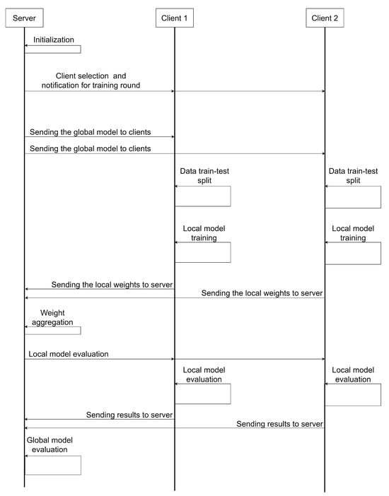
Figure 6.
Sequence diagram illustrating the interaction between the central server and two clients during a single training round.
- Server initialisation: The central server starts the training session, setting all the hyperparameters and preparing the global model. In this case, all experiments run 25 training rounds, with 5 local training epochs in each round, and a batch size of 64.
- Client selection and notification: The server selects a subset of clients (in this case, all clients are selected) to participate in the current training round.
- Distribution of the global model: The server sends the selected clients from the previous step a copy of the current global model weights.
- Splitting local data into train and test: Each client reserves 20% of their local data for a later test phase. This is only performed in the first round, maintaining the split for the rest of the rounds.
- Local model training: After splitting the data, each client trains their copy of the global model on their local train set. This training is performed for five epochs in each round. It is worth noting that, to prevent each local model from overfitting to the peculiarities of each client’s local data, dropout layers have been introduced in all trained model architectures. This ensures proper generalisation capacity of the global model.
- Aggregation of local model weights: After local training, clients send the local model weights to the server, where aggregation is performed using the Federated Average (FedAvg) strategy, which averages all local weights to update the global model weights. To ensure convergence, the global model weights are only updated if the average accuracy of all clients has improved compared to the previous round.
- Local evaluation of the global model: Once all local weights are aggregated and set as the new global model weights, they are sent back to the clients, who perform a local evaluation of the current global model on the local test data reserved in the first training round.
- Global model evaluation: After the local evaluation, the server performs its own evaluation of the global model on its own test set, which was extracted during the data preprocessing phase, explained in Section 2.2.
It is worth noting that, to maintain clarity in Figure 6, only 2 clients are represented, although 40 clients were used in all the experiments conducted. It was not possible to include a larger number due to computational resource constraints. However, the experiments conducted are perfectly transferable to an environment with a larger number of clients.
From the interaction sequence described, it can be deduced that there are two evaluation scenarios:
- -
- Global evaluation: The global model is evaluated on the server on its own test data, extracted according the explanation given in Section 2.2. These data are completely independent from the clients’ data, ensuring the global model is tested on data entirely different from those used in training.
- -
- Local or decentralised evaluation: The performance of the global model is also evaluated on the clients’ test sets (each test set constitutes 20% of each client’s local data), which are never seen during training, but are likely more similar to the train data.
In both scenarios, the precision, recall, accuracy, and f1-score metrics are measured on the test data. Moreover, confusion matrices are calculated to identify which attack classes the model performs best on and which ones are more challenging to detect.
Furthermore, the time taken by the whole federated learning process is measured, encompassing both the training phase and the evaluations on the test set. However, this time is entirely dependent on the machine on which the experiments are conducted. In this case, the specifications are as follows:
- -
- CPU: AMD Ryzen 7 8700 G with Radeon 780 M Graphics (8 cores, 16 threads). Frequency: 4.20 GHz.
- -
- RAM: 32 GB.
- -
- No GPU available.
Another key aspect of the implementation of federated learning is that clients may obtain local weights and gradients with opposing directions due to the heterogeneity of local data. This disparity can hinder, or even prevent, the convergence of the global model, as weight updates may cancel each other out. Therefore, to address this problem and mitigate its impact, it has been decided to allow several clients to use identical datasets. This approach promotes the alignment of gradient directions and facilitates a more stable and efficient convergence of the global model.
Finally, regarding weight aggregation, as already stated, the FedAvg strategy will be employed, which is a widely used method in federated learning that averages the weights of models trained on different clients. This method is chosen for its simplicity and effectiveness in various scenarios. However, it is important to note that the implications of using FedAvg under non-IID (non-Independent and Identically Distributed) data distributions can be significant. Non-IID data can lead to slower convergence and reduced model performance due to the heterogeneity of the data across clients. Therefore, to address data imbalance, undersampling techniques were applied, as already explained in Section 2.2.
3.2. MLP
Two different structures for MLP were tested. The first one consists of three hidden dense layers, with 256, 64, and 32 neurons, respectively, with dropout layers interspersed between the dense layers. Specifically, a 20% dropout is applied between the first and second hidden layers, a 10% dropout between the second and third hidden layers, and another 10% dropout after the third hidden layer, before the output layer. In the remainder of the paper, we will refer to this architecture as MLP-3HL. The second structure (which well be named as MLP-2HL) is simpler, consisting of two hidden layers with 128 and 32 neurons, respectively, with a 15% dropout layer interspersed between them.
Each of the two networks was trained and evaluated on the three different types of normalisation explained in Section 2.2, as well as on the three datasets with different numbers of lags, also detailed in Section 2.2. In this way, although MLPs are not inherently capable of benefiting from data with temporal structures or sequences, since each sample in the datasets is formed by the current message and the “lags” (1, 2, or 5) previous messages, it is possible to “force” the network to extract relationships between the different variables lagged over time.
It is worth noting that all experiments were repeated three times, both for this type of model and for GRUs and LSTMs, assigning different data partitions to the clients for greater robustness of the results. All the metrics presented are the averages obtained in the three repetitions of each experiment conducted.
Table 6 shows the results obtained by the architecture MLP-3HL, on each type of dataset and normalisation, in the global evaluation scenario, and Table 7 presents the results obtained by the same architecture but in the decentralised evaluation scenario. In view of both tables, it can be concluded that Min–Max normalisation yields the worst results by far, both in global and distributed evaluation. Between robust and standard normalisation, no clear performance difference is observed, although robust normalisation tends to achieve higher metrics in accuracy, but slightly lower in the rest of the metrics. Regarding the number of lags, models trained on the dataset with 2 lags per message tend to achieve better metrics compared to those trained on the datasets with 1 and 5 lags within the same normalisation technique. Moreover, in general, the metrics obtained in decentralised evaluation surpass those obtained in the corresponding global evaluation scenario, which is logical since the clients’ test data are more similar to those used for training than the server’s global evaluation data. However, since they are very close to each other, it is concluded that the models are generalising well to data that are quite different from those used for training.
Table 6.
Metrics obtained by the network MLP-3HL in the global evaluation scenario, where the global model was tested on server data, independent from client training data.
Table 7.
Metrics obtained by the network MLP-3HL in the local evaluation scenario, where the global model was tested on clients’ test data, unseen during training.
On the other hand, Table 8 presents the results obtained using each type of dataset and normalisation by the simpler architecture composed of two hidden layers in the global evaluation scenario, while Table 9 shows the results obtained in the decentralised evaluation scenario. It can be concluded, in view of the two tables, that this architecture achieves, generally, slightly better results than the previous one, especially for Min–Max normalisation, which, despite this, continues to present worse metrics than robust and standard normalisation, with the latter achieving the best metrics. The reduction in training time is also noteworthy, with a difference of more than 100 seconds in all cases, which is logical since the model to be trained is considerably simpler than the first architecture. As with the first network, the results in the decentralised scenario surpass those obtained in the global evaluation, but again, they are close and consistent with each other, presenting the same increasing and decreasing trends, once again demonstrating the model’s correct generalisation capability.
Table 8.
Metrics obtained by the network MLP-2HL in the global evaluation scenario, where the global model was tested on server data, independent from client training data.
Table 9.
Metrics obtained by the network MLP-2HL in the local evaluation scenario, where the global model was tested on clients’ test data, unseen during training.
Therefore, in view of the four tables of results obtained for the two MLP networks, although the metrics achieved by MLP-2HL in the global and local scenarios slightly surpass those obtained by MLP-3HL, the best MLP model is the one trained for standard normalisation with 2 lags, using the MLP-3HL architecture, which achieves an accuracy of 90.25% in the global scenario and 92.12% in the local scenario, presenting a difference of less than 2% between both scenarios, and with the rest of the metrics (precision, recall, and f1-score) above 90% in both cases. On the other hand, although the network trained for standard normalisation with 1 lag and the MLP-2HL architecture achieves a slightly higher accuracy of 90.37% in the global evaluation scenario, the rest of the metrics are below 89% in both the global and local scenarios, and, moreover, the difference in accuracy between both scenarios is higher, specifically 2.26%. Therefore, we choose as the best MLP model the network trained for standard normalisation with 2 lags, using the MLP-3HL architecture. Figure 7 and Figure 8 show, respectively, the confusion matrix obtained by this best MLP model on the global test set of the server, and the aggregated confusion matrix obtained as the average of all the confusion matrices obtained by the model on the local test data of the clients. To better understand the matrices, Table 10 shows which attack corresponds to each number.
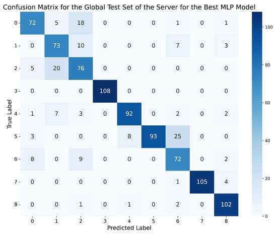
Figure 7.
Confusion matrix for the global test set of the server using the best MLP model (standard normalisation, 2 lags, MLP-3HL).

Figure 8.
Aggregated confusion matrix for the local test data of the clients using the best MLP model (standard normalisation, 2 lags, MLP-3HL).
Table 10.
Correspondence between the numbers on the axes of the confusion matrices and the attacks.
In the confusion matrix of the global evaluation scenario shown in Figure 7, it can be observed that the model tends to correctly classify all classes, with the highest number of errors occurring between the most similar classes, such as ‘Constant position’ (1) and ‘Constant position offset’ (2), with 20 errors, and between the latter and normal behaviour (0), with 18 errors. The classes ‘Constant speed’ (5) and ‘Constant speed offset’ (6) are also confused, with 25 errors.
On the other hand, regarding the confusion matrix depicted in Figure 8, and obtained by the model in the local evaluation scenario, it can be observed that, although the errors tend to occur in the same places as in the global evaluation scenario, it is noteworthy that, in this case, there is a significant proportion of errors where the model predicts an attack of type 2 (Constant position offset) when, in reality, the messages correspond to normal behaviour.
3.3. GRU
For GRU, a first architecture with two GRU layers was defined, the first (GRU-3L) with 128 neurons and the second with 64 neurons, followed by a dense layer of 128 neurons. A 20% dropout layer was introduced between the dense layer and the output layer. On the other hand, the second defined network (GRU-4L) also consists of two GRU layers, in this case with 64 and 32 neurons, followed by a dense layer of 32 neurons and another of 16, with a 10% dropout layer between the two dense layers.
Again, both types of architectures were tested on the three types of normalisation and datasets, with three repetitions per experiment to ensure consistent results.
Analogous to what was carried out for the MLP models, Table 11 and Table 12 present the average metrics of the three repetitions obtained by the GRU-3L network in the different experiments in the global evaluation scenario and in the decentralised evaluation scenario, respectively. In Table 11, it can be observed that the metrics achieved by the model in the global evaluation surpass those obtained by the two MLP architectures in the same global evaluation. In some cases, they even exceed the results of the MLPs in the decentralised evaluation, highlighting the better performance of neural networks capable of learning time series for this problem. Again, as with the MLPs, the metrics obtained by the model in the decentralised evaluation scenario surpass those obtained in the global evaluation. Furthermore, unlike what happened with the MLPs, there is no clear difference between the Min–Max normalisation and the other two, although the standard normalisation generally achieves the best results. As expected, the training times have doubled compared to those of the MLPs, as GRUs are considerably more complex. Once again, the precision and recall metrics are very similar to each other, indicating that the model has a good balance between the ability to correctly identify positive instances (recall) and the precision of those identifications (precision).
Table 11.
Metrics obtained by the network GRU-3L in the global evaluation scenario, where the global model was tested on server data, independent from client training data.
Table 12.
Metrics obtained by the network GRU-3L in the local evaluation scenario, where the global model was tested on clients’ test data, unseen during training.
Similarly, Table 13 and Table 14 present the metrics obtained in the two types of evaluation scenarios, global and decentralised, respectively, by the second network architecture, GRU-4L. In this case, the results slightly worsen compared to the GRU-3L architecture, although the same patterns are maintained. The metrics remain consistent between the two types of evaluation, global and local, and the standard normalisation again achieves better results than the Min–Max and robust normalisation. The training times are slightly reduced compared to GRU-3L, as this second architecture is slightly simpler than the previous one.
Table 13.
Metrics obtained by the network GRU-4L in the global evaluation scenario, where the global model was tested on server data, independent from client training data.
Table 14.
Metrics obtained by the network GRU-4L in the local evaluation scenario, where the global model was tested on clients’ test data, unseen during training.
If, once again, we choose a better GRU model based on the metrics obtained in the four tables, in this case, the best network is the one trained on the dataset with 5 lags and standard normalisation, using the GRU-3L architecture. This model achieved an accuracy of 93.5% in the global evaluation scenario, and 97.12% on the clients’ test data, with an accuracy difference of 3.62% between both scenarios. Moreover, all other metrics are above 95% in all cases. Therefore, this GRU model outperforms the best model chosen for the MLPs, demonstrating that, in this case, it is more appropriate to use networks with long-term memory capacity, as they are capable of capturing more complex temporal dependencies than those simply given by the number of lags, offering superior performance to the MLPs. Figure 9 and Figure 10 depict the confusion matrix obtained by this model on the global test set of the server, and the aggregated confusion matrix obtained by the model on all the local test data of the clients.
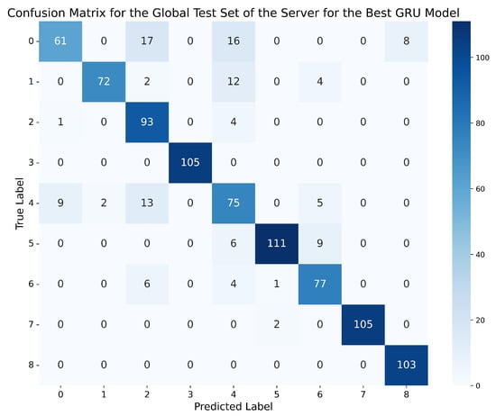
Figure 9.
Confusion matrix for the global test set of the server using the best GRU model (standard normalisation, 5 lags, GRU-3L).

Figure 10.
Aggregated confusion matrix for the local test data of the clients using the best GRU model (standard normalisation, 5 lags, GRU-3L).
In this case, the number of examples slightly differs from those in the matrices of Figure 7 and Figure 8, since both the global and local test sets are adapted to the dataset with 5 lags, as it proved to be the best for GRU networks, while for MLPs, the best dataset was the one with 2 lags. However, in the case of the confusion matrix obtained by the best GRU on the global scenario (Figure 9), it shows a total reduction in the number of errors made by the model between classes 2 (Constant position offset) and 1 (Constant position), decreasing from 20 errors obtained by the best MLP to 0. The same happens between classes 5 (Constant speed) and 6 (Constant speed offset), where, in this case, the best GRU reduces the 25 errors made by the best MLP to just 9. However, the confusion between classes 0 (Normal behaviour) and 2 (Constant position offset) remains almost unchanged, with only one less error in this case, but the number of errors between ‘Normal behaviour’ and class 4 (Random position offset) increases, reaching 16 in this case.
On the other hand, the average number of errors made on the local test data of different clients by the best GRU is significantly reduced between classes 2 (Constant position offset) and 0 (Normal behaviour), compared to the best MLP, decreasing from 308 errors for the MLP to 84 for the GRU. However, the number of errors in the GRU increases in class 4 (Random position offset), confusing it 121 times with ‘Normal behaviour’ and 109 times with attack 2 (Constant position offset).
3.4. LSTM
Regarding LSTMs, two distinct architectures were defined once again: LSTM-3L, composed of an LSTM layer with 128 neurons, connected to a dropout layer of 10%, followed by two dense layers of 64 and 32 neurons, respectively, with another dropout layer of 20% interspersed between them, and LSTM-4L, a slightly more complex network, consisting of two LSTM layers with 128 and 64 neurons, followed by a dense layer of 32 neurons, a dropout layer of 15%, and a final hidden dense layer of 16 neurons.
As with all previous networks, both architectures were evaluated three times, both globally and locally. Table 15 shows the average results obtained by the LSTM-3L network in the three evaluations on the global scenario, where it can be observed that, once again, standard normalisation considerably outperforms the other two, especially for 2 lags, which is the number of lags that presents the best results in the three types of normalisation, compared to the datasets with 1 and 5 lags. Likewise, comparing these metrics with those obtained by the same model in the local evaluation scenario, shown in Table 16, a consistency between the results achieved in both scenarios is observed once again, especially in the model trained with standard normalisation and the dataset with 2 lags, where there is practically no difference between the metrics shown in both tables, demonstrating that it is capable of making a perfect generalisation on the global test data of the server, despite having been trained with the different local data of the various clients.
Table 15.
Metrics obtained by the network LSTM-3L in the global evaluation scenario, where the global model was tested on server data, independent from client training data.
Table 16.
Metrics obtained by the network LSTM-3L in the local evaluation scenario, where the global model was tested on clients’ test data, unseen during training.
Concerning the LSTM-4L network, Table 17 and Table 18, the results are marginally worse compared to LSTM-3L, although, once again, the same patterns as in the previous case are maintained, with standard normalisation outperforming Min–Max and robust scaler, and the models trained on the dataset with 2 lags achieving better results than those trained on the datasets with 1 and 5 lags. Again, consistency is observed between the metrics obtained in the global and local evaluation scenarios, although, in this case, there is a greater difference between the two than in LSTM-3L, with discrepancies exceeding 7% in some cases.
Table 17.
Metrics obtained by the network LSTM-4L in the global evaluation scenario, where the global model was tested on server data, independent from client training data.
Table 18.
Metrics obtained by the network LSTM-4L in the local evaluation scenario, where the global model was tested on clients’ test data, unseen during training.
In this case, the best LSTM network was the one trained on the dataset with 2 lags, with standard normalisation and the LSTM-3L architecture, achieving an accuracy of 96.75% in the global evaluation scenario on the server’s dataset, and 96.93% in the local evaluation scenario on the clients’ local test data. It can be observed that this model not only obtains the best metrics compared to GRU and MLP, but also the closest metrics in both scenarios, with only a 0.18% difference, making it the model that best generalises to data different from those used for training. Furthermore, the precision, recall, and f1-score metrics are between 95.7% and 96%. Finally, Figure 11 and Figure 12 demonstrate that this model outperforms the best GRU and the best MLP, reducing classification errors compared to the previous models.
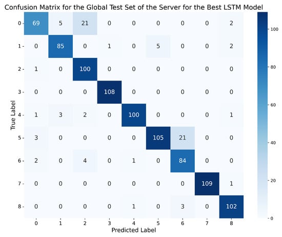
Figure 11.
Confusion matrix for the global test set of the server using the best LSTM model (standard normalisation, 2 lags, LSTM-3L).
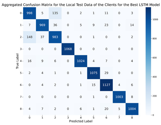
Figure 12.
Aggregated confusion matrix for the local test data of the clients using the best LSTM model (standard normalisation, 2 lags, LSTM-3L).
In Figure 11, it can be seen how the best LSTM reduces the errors between all classes in the global evaluation scenario to almost zero, except between ‘Normal behaviour’ (0) and class 2 (Constant position offset), where 21 errors are made, and between classes 5 (Constant speed) and 6 (Constant speed offset), where 21 errors also occur. It is worth noting that for the best GRU and the best MLP, a high number of errors were also made between these two pairs of classes.
For the confusion matrix obtained by the best LSTM in the local evaluation scenario, shown in Figure 12, a very significant reduction in the number of errors is observed, compared to both the best GRU and the best MLP. However, consistent with both previous models, the confusion between classes 0 and 2 is repeated, but much more reduced.
To better understand the repeated confusion between classes 0 and 2, and between classes 5 and 6, it is worth noting that the first two are considerably similar to each other, as class 2 simply differs from normal behaviour in that a constant offset is added to the position. Therefore, the dynamics or movement pattern (temporal variation, accelerations, etc.) remains very similar to that of the normal class. On the other hand, similarly, in class 5 there is a constant speed behaviour and in class 6 a constant offset is introduced in the speed, which, if introduced on a normal vehicle travelling at a constant speed for a certain time, can lead to confusion between the two classes.
Therefore, after analysing the results obtained by each type of network, it can be concluded that the best model is the LSTM-3L trained on the dataset with 2 lags and standard normalisation, outperforming both MLPs and GRUs.
3.5. Differential Privacy
As stated in Section 2.4, the differential privacy tests were only conducted on the final LSTM global model. To conduct these tests, three repetitions of the training of the best LSTM were performed again on the same dataset with 2 lags and standard normalisation. The results obtained are shown in Figure 13, where the X axis shows the different values of , and the Y axis shows the average accuracy percentage obtained for each type of noise (Laplace, Gaussian with , and Gaussian with ).
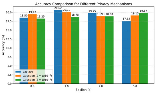
Figure 13.
Results of differential privacy tests on the final global LSTM model. The graph shows the average accuracy percentage for each type of noise (Laplace, Gaussian with , and Gaussian with ) across different values of .
It can be clearly seen that, in this case, for all types of noise tested, regardless of the values of or , differential privacy severely harms the model’s accuracy, achieving at most 20.62% in the best case, while without differential privacy, the best LSTM network achieved an accuracy of 96.75%.
3.6. Discussion
The results obtained in this study surpass those reported in [33], achieving an accuracy of 96.75% in classifying eight types of attacks plus normal behaviour, compared to the 93% achieved in their work, which only considered five types of attacks plus normal behaviour.
However, the results described in [30], where an accuracy of 99.99% was achieved following a centralised approach, were not exceeded. A possible explanation lies in the decision to remove identifiers as an input variable for training, as this measure prevents the model from learning specific associations between identifiers and types of attacks, which could lead to an artificial improvement in the results. Moreover, centralised learning schemes usually facilitate convergence, as the model is trained on all data at once, resulting in gradient updates that are consistent in the same direction, without multiple clients training different versions with gradients that may update in opposite directions and need to be aggregated to produce a global model, leading, therefore, to better performance metrics compared to distributed environments.
Furthermore, the evaluation methodology applied in this study, particularly in the global scenario, ensures that the test data are completely independent of the local training data of the clients, as they come from different vehicles.
On the other hand, while federated learning improves privacy compared to centralised approaches, it also presents vulnerabilities, such as poisoning attacks. However, there are multiple countermeasures proposed [57,58] to mitigate these attacks, notably the implementation of aggregation techniques resistant to Byzantine behaviours, among which there are options such as Multi-Krum, trimmed mean, or median-based aggregation. Another line of defence is the use of consistency verification and update validation techniques, which can be implemented through encryption mechanisms and consensus protocols adapted to distributed environments, to corroborate the integrity of the data sent by clients before integrating them into the global update.
4. Conclusions
The results obtained in the experiments conducted across this study demonstrated that LSTM networks outperformed both GRU and MLP, achieving an accuracy of 96.75% in detecting eight different types of intrusions from the VeReMi dataset, as well as differentiating these attacks from normal behaviour in vehicles. Therefore, it demonstrates the superior performance that Recurrent Neural Networks, capable of intrinsically working with sequences of temporal data, present compared to other structures like MLP, which, although capable of obtaining good results, especially considering that different preprocessing steps were applied to the datasets in the form of temporal lags to force better detection of relationships and temporal patterns between messages from different vehicles, achieve lower accuracy values.
On the other hand, among the normalisation methods compared, the metrics obtained by the different types of models conclude that, in this case, standard normalisation is the most appropriate, while Min–Max normalisation obtains the worst results in all cases. This is because, since the work was conducted on the VeReMi dataset, which collects speed and position measurements, there was a strong presence of outliers, especially in speed, which negatively affects Min–Max normalisation. By compressing all data into a range of 0 to 1, in the presence of extreme values, it compresses the values too much, making it difficult for neural networks to extract relationships.
Furthermore, it is worth noting that among the different detected attacks and behaviours, the main point of confusion occurs between classes 0 (Normal behaviour) and 2 (Constant position offset), as demonstrated by the different confusion matrices shown for the various models.
Finally, the application of differential privacy to the parameters of the clients’ local models, before sending them to the server for aggregation, had a severe impact on the model’s accuracy, regardless of the type of noise used (Laplace or Gaussian) and the values of their parameters and , reducing the accuracy from 96.75% for the best model to 20.62%.
With regard to future research directions, the main ones lie in the practical feasibility of the proposed system in real vehicular scenarios, where edge devices have limited computational and energy resources.
Particularly, the implementation of digital twins is proposed, as this would allow for replicating the environment and behaviour of each vehicle in a virtual environment, where the intrusion detection model could be executed and optimised. If the twins are kept properly isolated, in terms of communication and data, the integrity and confidentiality of the system would still be ensured.
On the other hand, the incorporation of specialised computing devices, such as TPUs or GPUs, in the vehicles themselves should also be studied, as these would allow such models to be hosted efficiently so that each node would be able to respond in real time to a threat.
Likewise, since training from scratch can be prohibitive in environments without access to processing units, the possibility of fine-tuning the pre-trained model using data from the vehicle in which the system is deployed is proposed. Furthermore, a much smaller amount of data would be needed compared to the volume used in this paper to train the model from scratch.
Finally, although 40 vehicles have been simulated in this study, it should also be taken into account that, for deployment, as the number of vehicles in the system increases, the volume of information exchanged and the frequency of model updates will also increase. To address this future avenue, the use of clustering is proposed, which consists of grouping vehicles into regional subnets, performing a first phase of local aggregation before transmitting updates to the central server. It could also be interesting to study techniques specific to FL, and deep learning in general, such as gradient compression, which simply consists of reducing the size of the clients being transmitted to decrease the necessary bandwidth, or asynchronous updating, which allows local model updates to be integrated at different times, without having to wait for all clients to finish training in the same round.
Other future research directions may focus on the study of other potential mitigation strategies, besides differential privacy, which in this case has had a negative impact on the model, such as adaptive noise injection or secure aggregation.
Author Contributions
M.Z.M.: Conceptualization, Methodology, Software, Formal analysis, Investigation, Resources, Data Curation, Writing—Original Draft, Writing—Review and Editing, Visualization. R.M.-P.: Writing—Review and Editing, Supervision, Project Administration, Funding Acquisition. A.F.S.G.: Writing—Review and Editing, Supervision, Project Administration, Funding Acquisition. All authors have read and agreed to the published version of the manuscript.
Funding
This paper has been supported by the EU Commission under the following project: DISTRIMUSE (GA 101139769). This paper was also supported by the Innovation Spanish Agency under the following projects: PROMETEO (Reference TSI-064200-2022-003) and Mas4Care (Reference TSI-065100-2023-006).
Institutional Review Board Statement
Not applicable.
Informed Consent Statement
Not applicable.
Data Availability Statement
The original data presented in the study are openly available in GitHub at https://github.com/miriozzy/Vehicle-Intrusion-Data-FL-LSTM (accessed on 3 April 2025).
Conflicts of Interest
The authors declare no conflicts of interest.
References
- Dhull, P.; Guevara, A.P.; Ansari, M.; Pollin, S.; Shariati, N.; Schreurs, D. Internet of Things networks: Enabling simultaneous wireless information and power transfer. IEEE Microw. Mag. 2022, 23, 39–54. [Google Scholar] [CrossRef]
- Rossini, R.; Lopez, L. Towards an European Open Continuum Reference Stack and Architecture. In Proceedings of the 2024 9th International Conference on Smart and Sustainable Technologies (SpliTech), Bol and Split, Croatia, 25–28 June 2024; IEEE: Piscataway, NJ, USA, 2024; pp. 1–5. [Google Scholar] [CrossRef]
- Griffith, D. Innovation at the edge: IoT 2.0. In Proceedings of the 2022 IEEE Asian Solid-State Circuits Conference (A-SSCC), Taipei, Taiwan, 6–9 November 2022; IEEE: Piscataway, NJ, USA, 2022; pp. 2–3. [Google Scholar] [CrossRef]
- Chandy, A. A review on iot based medical imaging technology for healthcare applications. J. Innov. Image Process. (JIIP) 2019, 1, 51–60. [Google Scholar] [CrossRef]
- Sadoughi, F.; Behmanesh, A.; Sayfouri, N. Internet of things in medicine: A systematic mapping study. J. Biomed. Inform. 2020, 103, 103383. [Google Scholar] [CrossRef]
- Ranjan, R.; Sahana, B.C. A Comprehensive Roadmap for Transforming Healthcare from Hospital-Centric to Patient-Centric Through Healthcare Internet of Things (IoT). Eng. Sci. 2024, 30, 1175. [Google Scholar] [CrossRef]
- Abdulmalek, S.; Nasir, A.; Jabbar, W.A.; Almuhaya, M.A.; Bairagi, A.K.; Khan, M.A.M.; Kee, S.H. IoT-based healthcare-monitoring system towards improving quality of life: A review. Healthcare 2022, 10, 1993. [Google Scholar] [CrossRef] [PubMed]
- Javaid, M.; Haleem, A.; Singh, R.P.; Rab, S.; Suman, R. Upgrading the manufacturing sector via applications of Industrial Internet of Things (IIoT). Sensors Int. 2021, 2, 100129. [Google Scholar] [CrossRef]
- Lampropoulos, G.; Siakas, K.; Anastasiadis, T. Internet of things in the context of industry 4.0: An overview. Int. J. Entrep. Knowl. 2019, 7, 4–19. [Google Scholar] [CrossRef]
- Li, Q.; Yang, Y.; Jiang, P. Remote monitoring and maintenance for equipment and production lines on industrial internet: A literature review. Machines 2022, 11, 12. [Google Scholar] [CrossRef]
- Martínez, M.Z.; Silveira, L.H.M.D.; Marin-Perez, R.; Gomez, A.F.S. Development of a Neural Network System for Predicting Topsoil Moisture Using Remote Sensing and Rainfall Forecast Data. In Proceedings of the 2024 4th International Conference on Embedded & Distributed Systems (EDiS), Bechar, Algeria, 3–5 November 2024; pp. 249–254. [Google Scholar] [CrossRef]
- Zambudio Martínez, M.; Silveira, L.H.M.d.; Marin-Perez, R.; Gomez, A.F.S. Development and Comparison of Artificial Neural Networks and Gradient Boosting Regressors for Predicting Topsoil Moisture Using Forecast Data. AI 2025, 6, 41. [Google Scholar] [CrossRef]
- Placidi, P.; Morbidelli, R.; Fortunati, D.; Papini, N.; Gobbi, F.; Scorzoni, A. Monitoring Soil and Ambient Parameters in the IoT Precision Agriculture Scenario: An Original Modeling Approach Dedicated to Low-Cost Soil Water Content Sensors. Sensors 2021, 21, 5110. [Google Scholar] [CrossRef]
- Ananthi, N.; Divya, J.; Divya, M.; Janani, V. IoT based smart soil monitoring system for agricultural production. In Proceedings of the 2017 IEEE Technological Innovations in ICT for Agriculture and Rural Development (TIAR), Chennai, India, 7–8 April 2017; IEEE: Piscataway, NJ, USA, 2017; pp. 209–214. [Google Scholar] [CrossRef]
- Ghosh, R.K.; Banerjee, A.; Aich, P.; Basu, D.; Ghosh, U. Intelligent IoT for automotive industry 4.0: Challenges, opportunities, and future trends. In Intelligent Internet of Things for Healthcare and Industry; Springer: Berlin/Heidelberg, Germany, 2022; pp. 327–352. [Google Scholar] [CrossRef]
- Krasniqi, X.; Hajrizi, E. Use of IoT technology to drive the automotive industry from connected to full autonomous vehicles. IFAC-PapersOnLine 2016, 49, 269–274. [Google Scholar] [CrossRef]
- Pourrahmani, H.; Yavarinasab, A.; Zahedi, R.; Gharehghani, A.; Mohammadi, M.H.; Bastani, P. The applications of Internet of Things in the automotive industry: A review of the batteries, fuel cells, and engines. Internet Things 2022, 19, 100579. [Google Scholar] [CrossRef]
- Khayyam, H.; Javadi, B.; Jalili, M.; Jazar, R.N. Artificial intelligence and internet of things for autonomous vehicles. In Nonlinear Approaches in Engineering Applications: Automotive Applications of Engineering Problems; Springer International Publishing: Cham, Germany, 2020; pp. 39–68. [Google Scholar] [CrossRef]
- Biswas, A.; Wang, H.C. Autonomous Vehicles Enabled by the Integration of IoT, Edge Intelligence, 5G, and Blockchain. Sensors 2023, 23, 1963. [Google Scholar] [CrossRef] [PubMed]
- Khattak, Z.H.; Smith, B.L.; Fontaine, M.D. Cyberattack Monitoring Architectures for Resilient Operation of Connected and Automated Vehicles. IEEE Open J. Intell. Transp. Syst. 2024, 5, 322–341. [Google Scholar] [CrossRef]
- Talpur, A.; Gurusamy, M. Machine learning for security in vehicular networks: A comprehensive survey. IEEE Commun. Surv. Tutorials 2021, 24, 346–379. [Google Scholar] [CrossRef]
- Demestichas, K.; Alexakis, T.; Peppes, N.; Adamopoulou, E. Comparative Analysis of Machine Learning-Based Approaches for Anomaly Detection in Vehicular Data. Vehicles 2021, 3, 171–186. [Google Scholar] [CrossRef]
- Jabbar, R.; Kharbeche, M.; Al-Khalifa, K.; Krichen, M.; Barkaoui, K. Blockchain for the Internet of Vehicles: A Decentralized IoT Solution for Vehicles Communication Using Ethereum. Sensors 2020, 20, 3928. [Google Scholar] [CrossRef]
- Shrestha, R.; Nam, S.Y.; Bajracharya, R.; Kim, S. Evolution of V2X Communication and Integration of Blockchain for Security Enhancements. Electronics 2020, 9, 1338. [Google Scholar] [CrossRef]
- Xun, Y.; Zhao, Y.; Liu, J. VehicleEIDS: A novel external intrusion detection system based on vehicle voltage signals. IEEE Internet Things J. 2022, 9, 2124–2133. [Google Scholar] [CrossRef]
- Tanaka, D.; Yamada, M.; Kashima, H.; Kishikawa, T.; Haga, T.; Sasaki, T. In-vehicle network intrusion detection and explanation using density ratio estimation. In Proceedings of the 2019 IEEE Intelligent Transportation Systems Conference (ITSC), Auckland, New Zealand, 27–30 October 2019; IEEE: Piscataway, NJ, USA, 2019; pp. 2238–2243. [Google Scholar] [CrossRef]
- Wu, W.; Huang, Y.; Kurachi, R.; Zeng, G.; Xie, G.; Li, R.; Li, K. Sliding window optimized information entropy analysis method for intrusion detection on in-vehicle networks. IEEE Access 2018, 6, 45233–45245. [Google Scholar] [CrossRef]
- Al-Jarrah, O.Y.; Maple, C.; Dianati, M.; Oxtoby, D.; Mouzakitis, A. Intrusion detection systems for intra-vehicle networks: A review. IEEE Access 2019, 7, 21266–21289. [Google Scholar] [CrossRef]
- Zhang, L.; Yan, X.; Ma, D. A binarized neural network approach to accelerate in-vehicle network intrusion detection. IEEE Access 2022, 10, 123505–123520. [Google Scholar] [CrossRef]
- Alladi, T.; Kohli, V.; Chamola, V.; Yu, F.R. A deep learning based misbehavior classification scheme for intrusion detection in cooperative intelligent transportation systems. Digit. Commun. Netw. 2023, 9, 1113–1122. [Google Scholar] [CrossRef]
- So, S.; Sharma, P.; Petit, J. Integrating plausibility checks and machine learning for misbehavior detection in VANET. In Proceedings of the 2018 17th IEEE International Conference on Machine Learning and Applications (ICMLA), Orlando, FL, USA, 17–20 December 2018; IEEE: Piscataway, NJ, USA, 2018; pp. 564–571. [Google Scholar] [CrossRef]
- Van Der Heijden, R.W.; Lukaseder, T.; Kargl, F. Veremi: A dataset for comparable evaluation of misbehavior detection in vanets. In Proceedings of the Security and Privacy in Communication Networks: 14th International Conference, SecureComm 2018, Singapore, Singapore, 8–10 August 2018; Proceedings, Part I. Springer: Berlin/Heidelberg, Germany, 2018; pp. 318–337. [Google Scholar] [CrossRef]
- Campos, E.M.; Hernandez-Ramos, J.L.; Vidal, A.G.; Baldini, G.; Skarmeta, A. Misbehavior detection in intelligent transportation systems based on federated learning. Internet Things 2024, 25, 101127. [Google Scholar] [CrossRef]
- Medlin, K.; Leyffer, S.; Raghavan, K. A Bilevel Optimization Framework for Imbalanced Data Classification. arXiv 2024. [Google Scholar] [CrossRef]
- Ramsauer, A.; Baumann, P.M.; Lex, C. The Influence of Data Preparation on Outlier Detection in Driveability Data. SN Comput. Sci. 2021, 2, 222. [Google Scholar] [CrossRef]
- Patro, S. Normalization: A Preprocessing Stage. CoRR 2015, abs/1503.06462. [Google Scholar] [CrossRef]
- Izonin, I.; Tkachenko, R.; Shakhovska, N.; Ilchyshyn, B.; Singh, K.K. A Two-Step Data Normalization Approach for Improving Classification Accuracy in the Medical Diagnosis Domain. Mathematics 2022, 10, 1942. [Google Scholar] [CrossRef]
- Popescu, M.C.; Balas, V.E.; Perescu-Popescu, L.; Mastorakis, N. Multilayer perceptron and neural networks. WSEAS Trans. Circuits Syst. 2009, 8, 579–588. [Google Scholar]
- Murtagh, F. Multilayer perceptrons for classification and regression. Neurocomputing 1991, 2, 183–197. [Google Scholar] [CrossRef]
- Pavani, K.; Damodaram, A. Intrusion detection using MLP for MANETs. In Proceedings of the Third International Conference on Computational Intelligence and Information Technology (CIIT 2013). The Institution of Engineering and Technology, Mumbai, India, 18–19 October 2013; pp. 440–444. [Google Scholar] [CrossRef]
- Amato, F.; Mazzocca, N.; Moscato, F.; Vivenzio, E. Multilayer perceptron: An intelligent model for classification and intrusion detection. In Proceedings of the 2017 31st International conference on advanced information networking and applications workshops (WAINA), Taipei, Taiwan, 27–29 March 2017; pp. 686–691. [Google Scholar] [CrossRef]
- Ahmad, I.; Abdullah, A.; Alghamdi, A.; Alnfajan, K.; Hussain, M. Intrusion detection using feature subset selection based on MLP. Sci. Res. Essays 2011, 6, 6804–6810. [Google Scholar] [CrossRef]
- Sanmorino, A.; Setiawan, H.; Coyanda, J.R. The utilization o machine learning for network intrusion detection systems. Inform. Autom. Pomiary Gospod. Ochr. Środowiska 2024, 14, 86–89. [Google Scholar] [CrossRef]
- Dey, R.; Salem, F.M. Gate-variants of gated recurrent unit (GRU) neural networks. In Proceedings of the 2017 IEEE 60th international midwest symposium on circuits and systems (MWSCAS), IEEE, Boston, MA, USA, 6–9 August 2017; pp. 1597–1600. [Google Scholar] [CrossRef]
- Zhang, Y.; Xiong, X.; Xiao, L.; Li, J.; Luo, R.; Zhang, J.; Zhang, H. Intrusion Detection Model Based on Recursive Gated Convolution and Bidirectional Gated Recurrent Units. In Proceedings of the 2024 IEEE International Conference on Smart Internet of Things (SmartIoT), Shenzhen, China, 14–16 November 2024; pp. 433–438. [Google Scholar] [CrossRef]
- Faiq Kamel, F.; Salih Mahdi, M. Intrusion Detection Systems Based on RNN and GRU Models using CSE-CIC-IDS2018 Dataset in AWS Cloud. J. Qadisiyah Comput. Sci. Math. 2024, 16, 141–160. [Google Scholar] [CrossRef]
- Panggabean, C.; Venkatachalam, C.; Shah, P.; John, S.; Devi, P.R.; Venkatachalam, S. Intelligent DoS and DDoS Detection: A Hybrid GRU-NTM Approach to Network Security. In Proceedings of the 2024 5th International Conference on Smart Electronics and Communication (ICOSEC), Trichy, India, 18–20 September 2024; IEEE: Piscataway, NJ, USA, 2024; pp. 658–665. [Google Scholar] [CrossRef]
- Graves, A. Long Short-Term Memory. Supervised Seq. Label. Recurr. Neural Netw. 2012, 385, 37–45. [Google Scholar] [CrossRef]
- Hochreiter, S.; Schmidhuber, J. Long Short-term Memory. Neural Comput. 1997, 9, 1735–1780. [Google Scholar] [CrossRef]
- Greff, K.; Srivastava, R.K.; Koutník, J.; Steunebrink, B.R.; Schmidhuber, J. LSTM: A Search Space Odyssey. IEEE Trans. Neural Netw. Learn. Syst. 2017, 28, 2222–2232. [Google Scholar] [CrossRef]
- Khan, M.A.; Karim, M.R.; Kim, Y. A Scalable and Hybrid Intrusion Detection System Based on the Convolutional-LSTM Network. Symmetry 2019, 11, 583. [Google Scholar] [CrossRef]
- Laghrissi, F.; Douzi, S.; Douzi, K.; Hssina, B. Intrusion detection systems using long short-term memory (LSTM). J. Big Data 2021, 8, 65. [Google Scholar] [CrossRef]
- Kumar, G.S.; Premalatha, K.; Maheshwari, G.U.; Kanna, P.R.; Vijaya, G.; Nivaashini, M. Differential privacy scheme using Laplace mechanism and statistical method computation in deep neural network for privacy preservation. Eng. Appl. Artif. Intell. 2024, 128, 107399. [Google Scholar] [CrossRef]
- El Ouadrhiri, A.; Abdelhadi, A. Differential privacy for deep and federated learning: A survey. IEEE Access 2022, 10, 22359–22380. [Google Scholar] [CrossRef]
- Sarathy, R.; Muralidhar, K. Evaluating Laplace noise addition to satisfy differential privacy for numeric data. Trans. Data Priv. 2011, 4, 1–17. [Google Scholar]
- Beutel, D.J.; Topal, T.; Mathur, A.; Qiu, X.; Fernandez-Marques, J.; Gao, Y.; Sani, L.; Li, K.H.; Parcollet, T.; de Gusmão, P.P.B.; et al. Flower: A friendly federated learning research framework. CoRR 2020, abs/2007.14390. [Google Scholar] [CrossRef]
- Xia, F.; Cheng, W. A survey on privacy-preserving federated learning against poisoning attacks. Clust. Comput. 2024, 27, 13565–13582. [Google Scholar] [CrossRef]
- Zhang, C.; Yang, S.; Mao, L.; Ning, H. Anomaly detection and defense techniques in federated learning: A comprehensive review. Artif. Intell. Rev. 2024, 57, 150. [Google Scholar] [CrossRef]
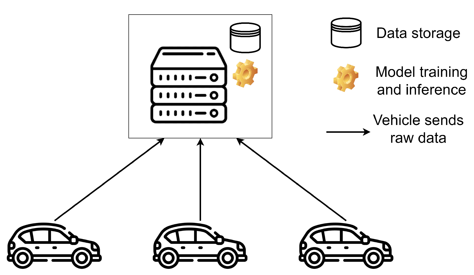
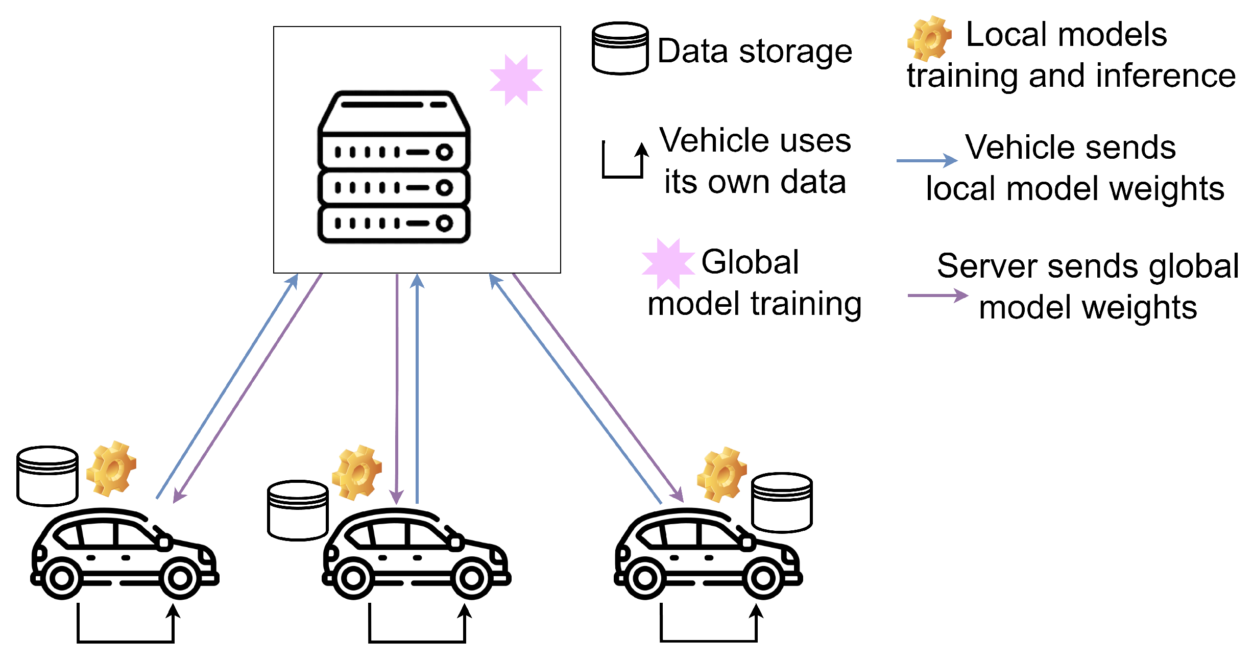
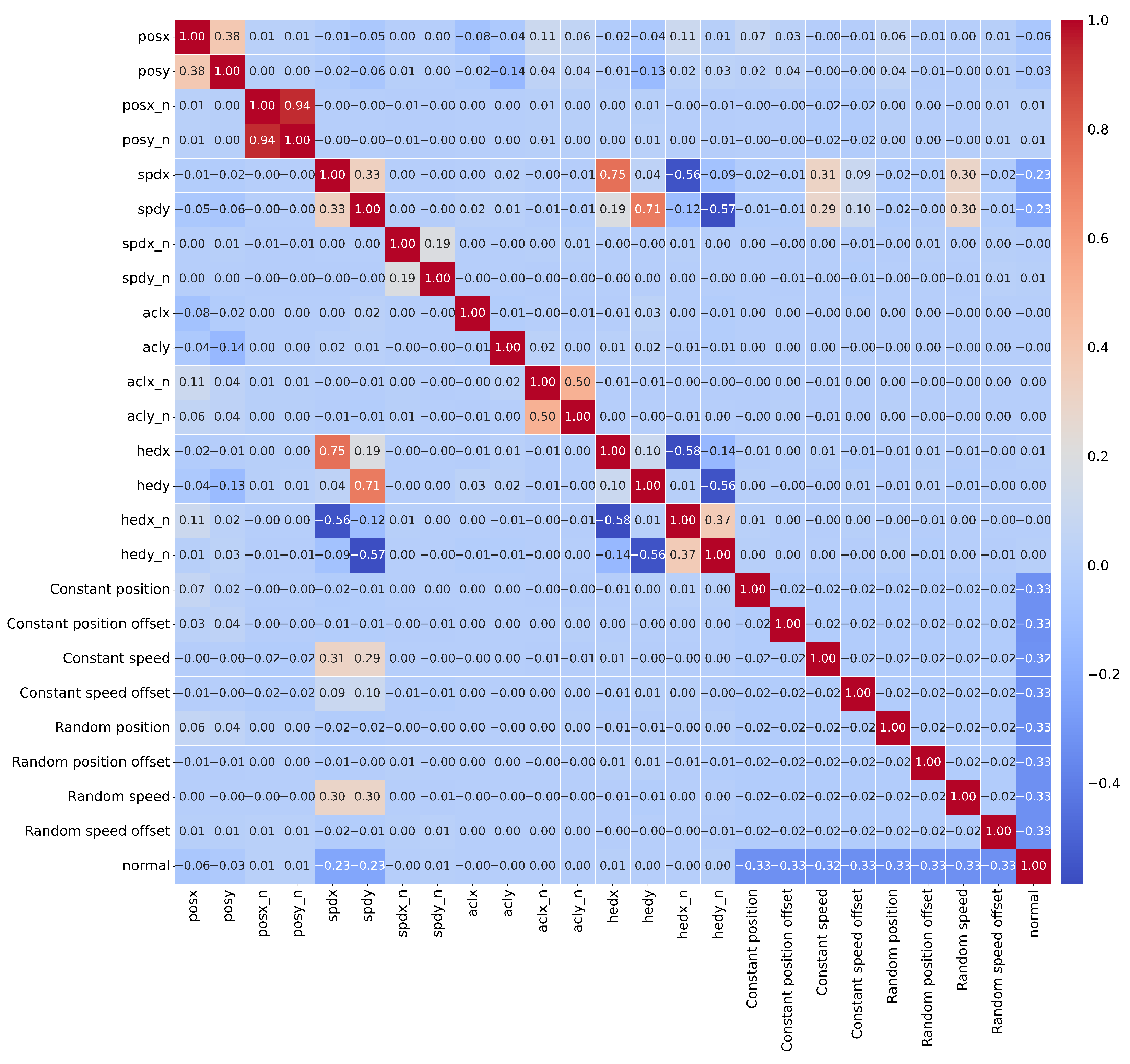
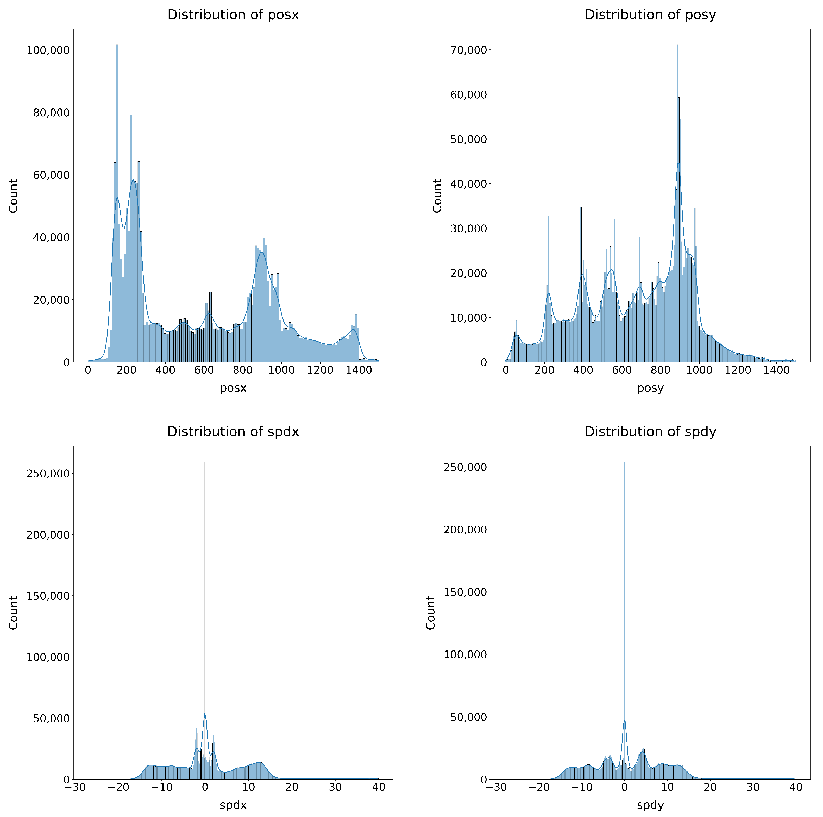
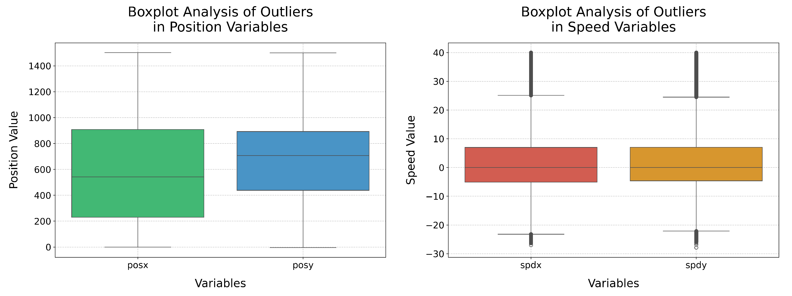
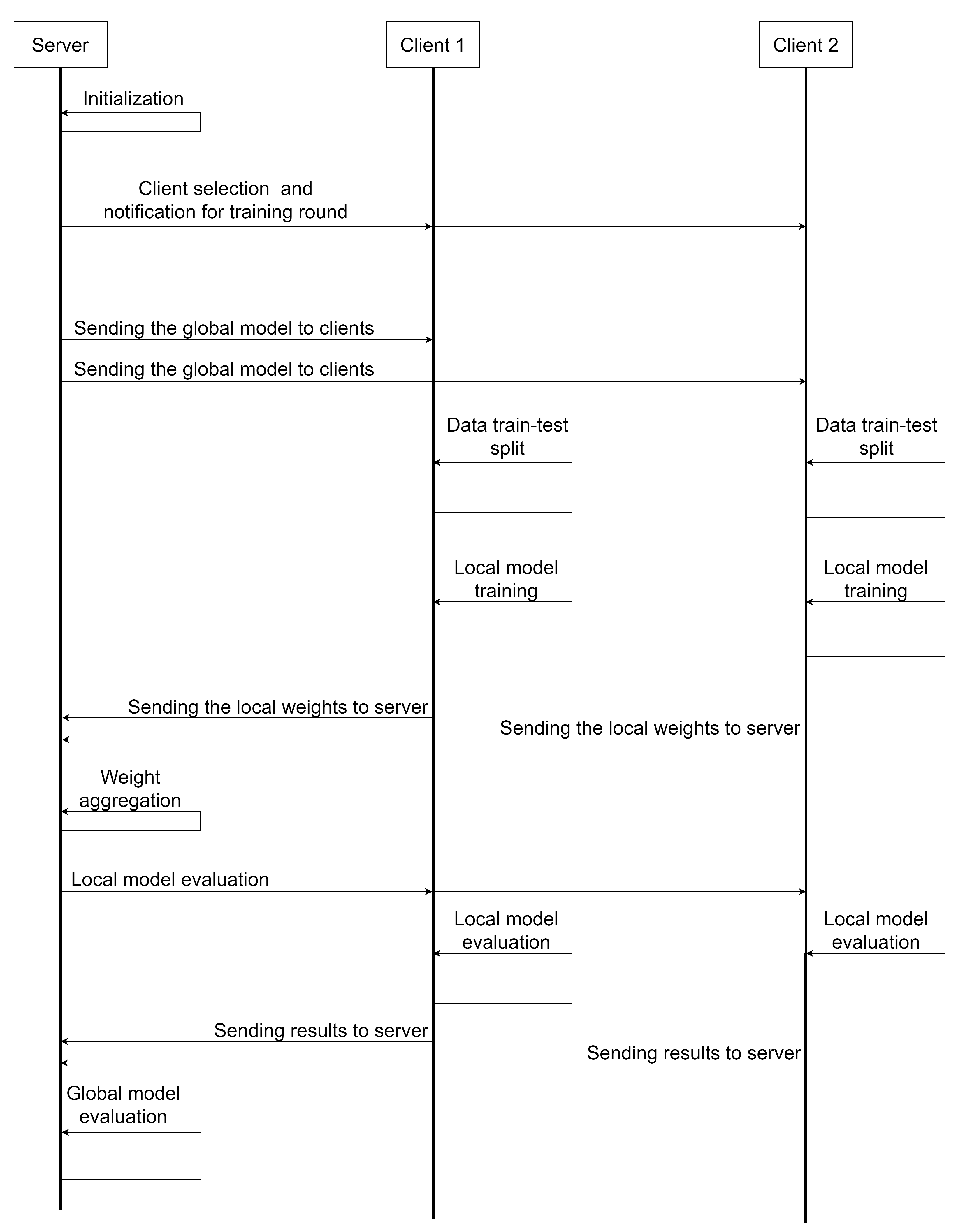

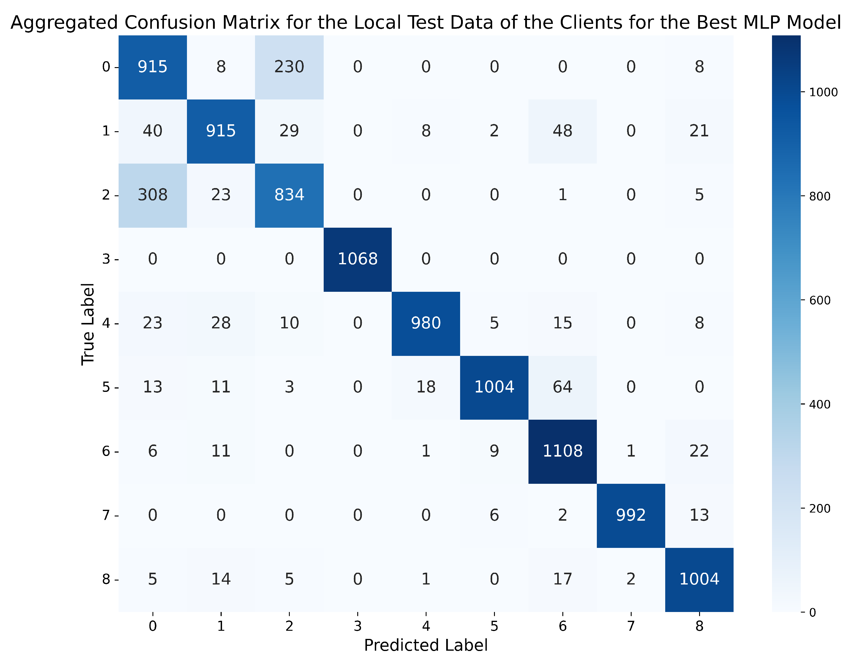

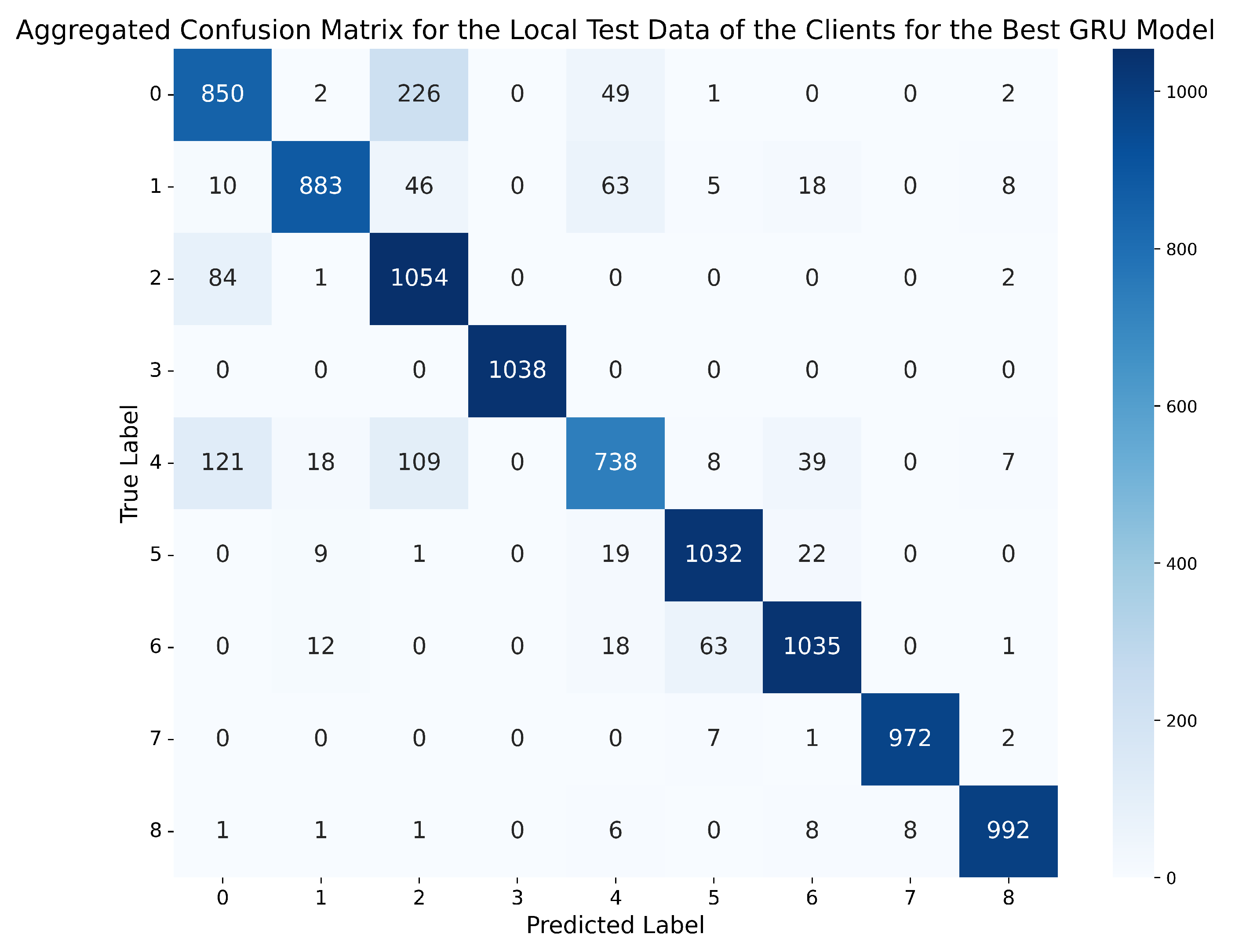

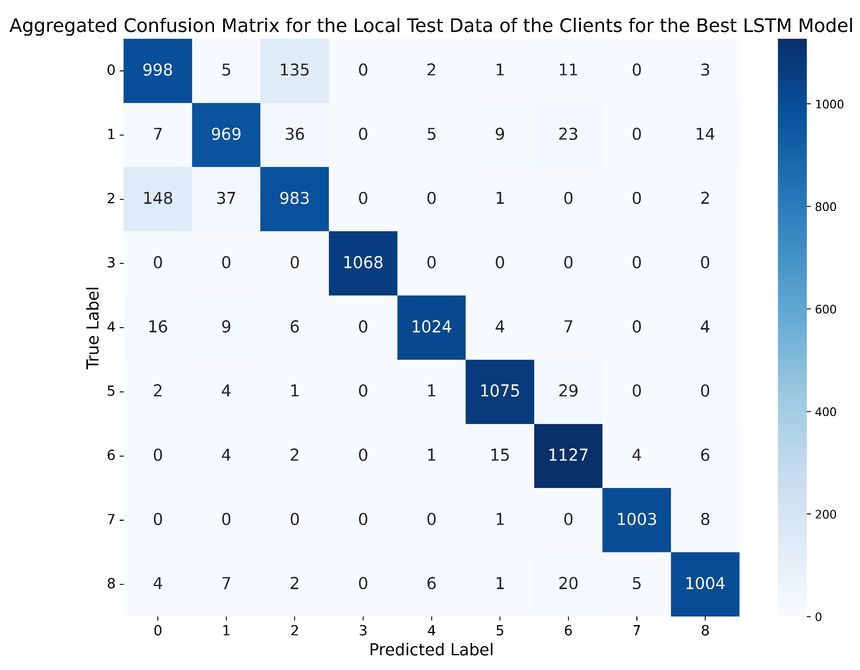
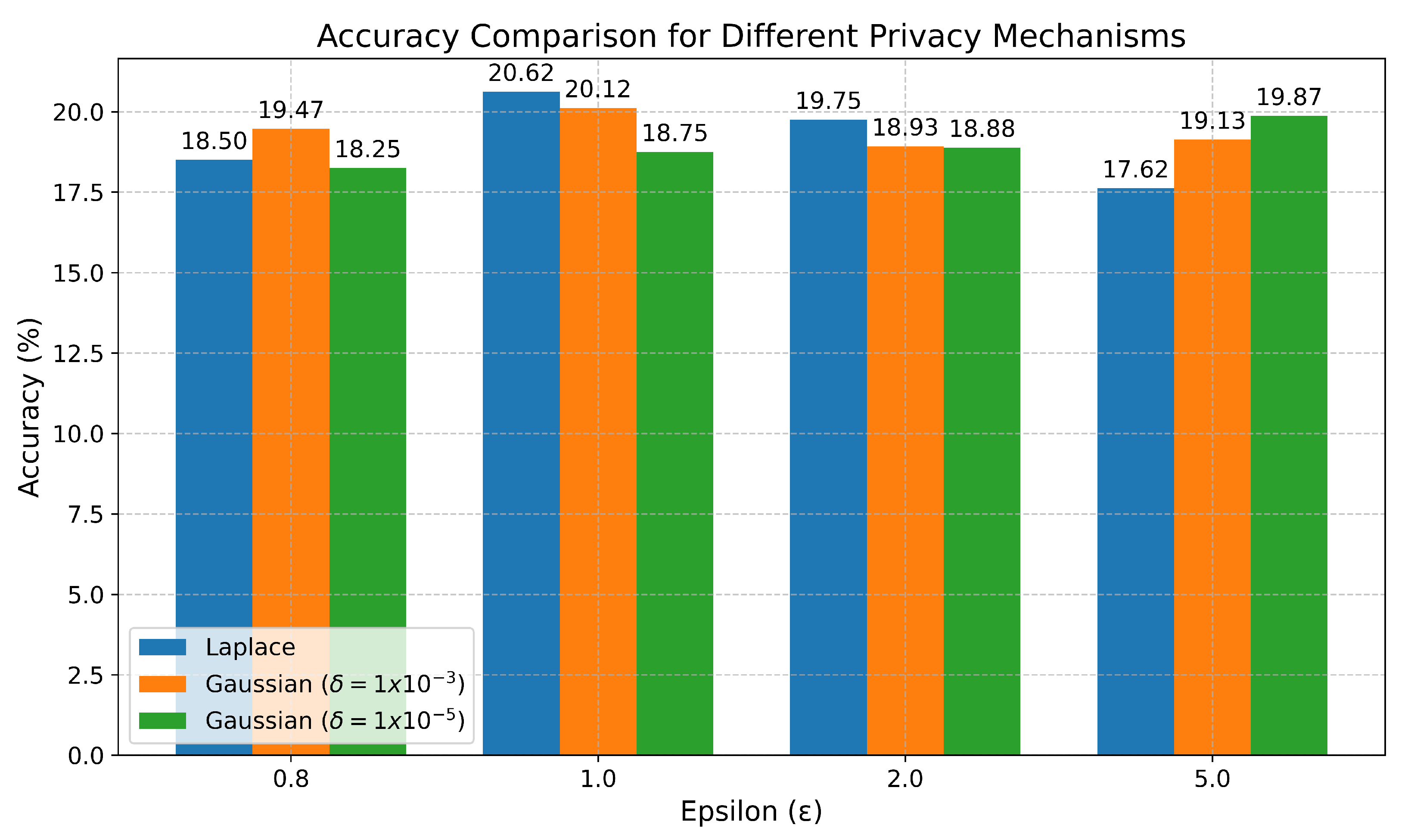
Disclaimer/Publisher’s Note: The statements, opinions and data contained in all publications are solely those of the individual author(s) and contributor(s) and not of MDPI and/or the editor(s). MDPI and/or the editor(s) disclaim responsibility for any injury to people or property resulting from any ideas, methods, instructions or products referred to in the content. |
© 2025 by the authors. Licensee MDPI, Basel, Switzerland. This article is an open access article distributed under the terms and conditions of the Creative Commons Attribution (CC BY) license (https://creativecommons.org/licenses/by/4.0/).