Active Distribution Network Source–Network–Load–Storage Collaborative Interaction Considering Multiple Flexible and Controllable Resources

Abstract

In the context of rapid advancement of smart cities, a distribution network (DN) serving as the backbone of urban operations is a way to confront multifaceted challenges that demand innovative solutions. Central among these, it is imperative to optimize resource allocation and enhance the efficient utilization of diverse energy sources, with particular emphasis on seamless integration of renewable energy systems into existing infrastructure. At the same time, considering that the traditional power system’s “rigid”, instantaneous, dynamic, and balanced law of electricity, “source-load”, is difficult to adapt to the grid-connection of a high proportion of distributed generations (DGs), the collaborative interaction of multiple flexible controllable resources, like flexible loads, are able to supplement the power system with sufficient “flexibility” to effectively alleviate the uncertainty caused by intermittent fluctuations in new energy. Therefore, an active distribution network (ADN) intraday, reactive, power optimization-scheduling model is designed. The dynamic reactive power collaborative interaction model, considering the integration of DG, energy storage (ES), flexible loads, as well as reactive power compensators into the IEEE 33-node system, is constructed with the goals of reducing intraday network losses, keeping voltage deviations to a minimum throughout the day, and optimizing static voltage stability in an active distribution network. Simulation outcomes for an enhanced IEEE 33-node system show that coordinated operation of source–network–load–storage effectively reduces intraday active power loss, improves voltage regulation capability, and achieves secure and reliable operation under ADN. Therefore, it will contribute to the construction of future smart city power systems to a certain extent.

1. Introduction

As of 2022, China’s coal consumption still accounts for 56.2% of the total energy consumption. In order to actively respond to the “dual carbon” goal and improve the proportion and efficiency of new energy utilization in smart cities, the domestic energy structure system urgently needs to be adjusted, and DG is also required to make further breakthroughs and progress [1,2]. As of December 2023, the capacity of a newly installed PV has increased to 609.49 gigawatts, an increase of 55.2% compared to the previous year. At the same time, newly installed wind energy has also achieved a significant milestone of 441.34 gigawatts, an increase of 20.7% compared to the previous year. As the “dual carbon” goal advances further, together with an increasing demand for the construction of smart cities, the rapid increase in the installed capacity of DGs also promoted the development of the energy storage industry [3,4]. However, the increase in the grid-connected capacity of DG can introduce numerous challenges to traditional distribution networks. Firstly, the volatility and intermittency of new energy will significantly increase the difficulty of grid planning and operation [5]; secondly, it greatly increases the possibility of uneven distribution of power flow, which hinders the security and stability of the power grid [6]; finally, frequent start–stops, as well as a lack of unified scheduling and planning, have increased the impact and wear on traditional power grid equipment. Based on the above challenges, active distribution network technology has emerged. ADN, with its excellent energy management strategy, achieves coordinated control over a series of flexible and controllable resources like DGs, ESs, and flexible loads to maximize the utilization of power grid resources and properly handle the aforementioned challenges [7,8].

Reactive voltage control guarantees secure and stable functioning of ADN. As such, many scholars focus on maximizing the coordinated development of flexible and controllable resources to enhance the reactive voltage dispatch capabilities [9]. The reactive power optimization in traditional distribution networks utilizes integrated planning of reactive power compensation equipment and transformer taps to reduce network losses [10,11]. With the increasing complexity of power systems, many scholars are actively exploring reactive power optimization and loss reduction measures that are more suitable for new power systems. Reference [12] proposed an approach driven by demand-side response, as well as designed a hybrid coevolutionary algorithm for solving it, effectively improving the reactive power compensation effect, as well as user satisfaction of DN. Reference [13] optimized the dynamic reactive power of ADN containing solid-state transformers, effectively solving the problems of voltage instability and increased active power loss caused by the integration of distributed generations. Reference [14] studied the reactive power optimization problem of DN, taking into account source–network–load–storage. A control method based on price driven demand response and energy storage system (ESS) coordination was proposed to enhance the safety of the system. Reference [15] found that using flexible interconnected devices (such as VSCs) to transform traditional distribution networks into AC/DC hybrid networks can enhance network flexibility and alleviate power quality issues caused by new energy and load integration.

An innovative method for renewable energy forecasting, grounded in optimized SVM parameters, as well as targeted meteorological feature selection, is proposed in reference [16] to address the random fluctuation of DG on the source side. This method can significantly improve the precision of DG prediction models as well as offer robust backing for the consumption and utilization of DG. The focus of research on the network side is on minimizing system losses, reducing voltage deviations, and ensuring stable system operation as much as possible. Reference [17] found that wind turbines can significantly reduce power losses and improve grid performance when providing reactive power, providing theoretical support for the planning and operation of DN. From the perspective of the load side, the flexible adjustment of flexible loads is beneficial for improving the response speed of the power grid to adapt to the random fluctuations of DG while maintaining optimal equilibrium between energy generation and consumption. Reference [18] established a flexible resource interaction model, including distributed photovoltaics (DPV), energy storage systems, and flexible loads. These flexible and controllable resources achieve reactive power interactions with the distribution network through different reactive power regulation capabilities and their coordination with each other. Reference [19] delves into the reactive power optimization problem of flexible controllable resources in active distribution networks, proposing the use of time-of-use electricity prices as the basis to reduce system network loss and voltage fluctuation by coordinating the comprehensive output of DG and ESS, along with reactive power compensators.

The integration of DG into the network and flexible participation of flexible loads, together with the integration of ESS, will inevitably contribute to richer strategies for reactive power dispatch in the power grid. The study systematically investigates the operational attributes of both the aforementioned heterogeneous flexible controllable resources and conventional reactive power compensation devices, with a dual optimization focus on enhancing system economic efficiency and ensuring operational stability. Combining a series of constraints, such as new energy output, energy storage characteristics, flexible load operation status, and traditional reactive power compensation equipment, a collaborative interaction model of “source-network-load-storage” under ADN, considering multiple flexible controllable resources, is finally designed. Finally, the Hybrid Whale Grey Wolf Algorithm (H-WOA-GWO) is used for computation and finding a solution. This algorithm combines the excellent local search ability of the Grey Wolf Optimizer (GWO) and the powerful global search ability and exploration of unknown regions of the Whale Optimization Algorithm (WOA), and has significant advantages in handling different types of decision variables and solving dynamic optimization problems with a large and complex number of decision variables. Modeling outcomes indicate that ADN has a stronger reactive voltage regulation capability and lower intraday active power network loss under the collaborative interaction of source–network–load–storage, while achieving reliable and steady operation under ADN and fulfilling the function of “peak shaving and valley filling”.

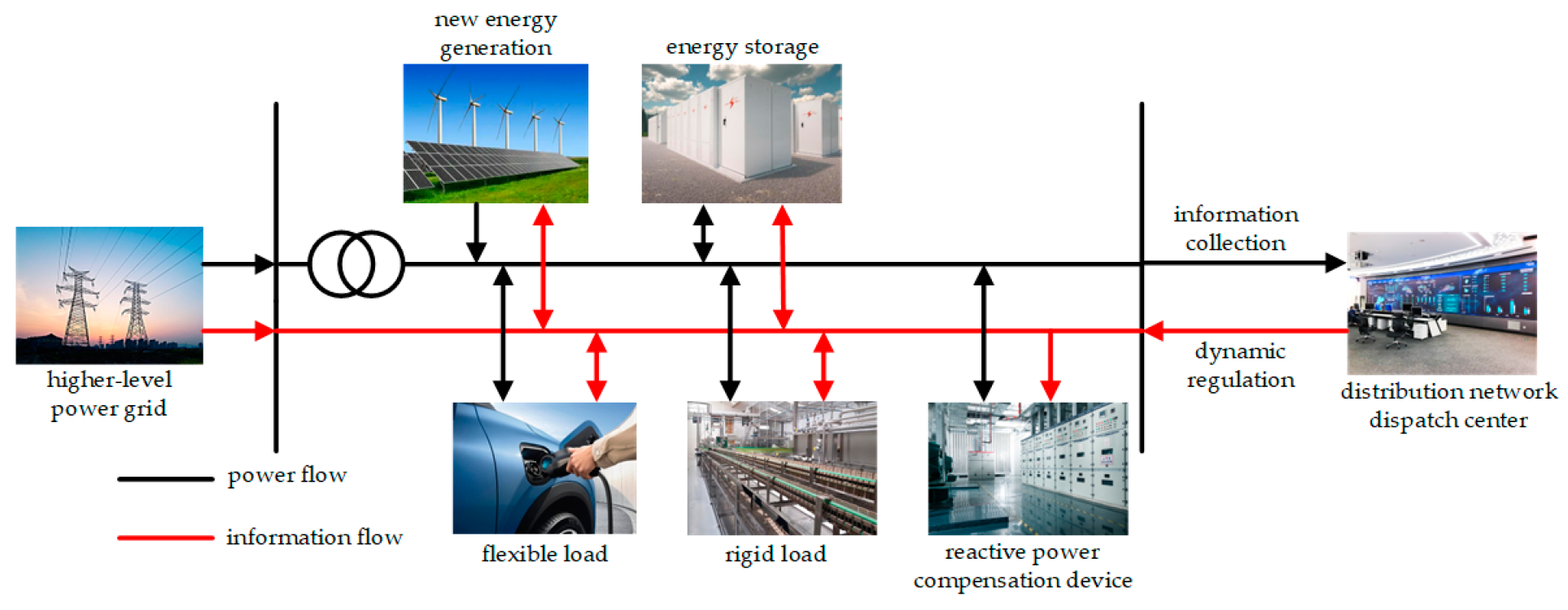
2. ADN Architecture

The most significant difference between active distribution networks and traditional distribution networks lies in their controllability and flexibility, which helps to achieve optimized scheduling and interaction in the power system. The interaction paths between each component unit in ADN, higher-level power grid, and distribution network dispatch center are mainly power flow and information flow. The former involves the actual transmission process of electrical energy, while the latter refers to the management functions of monitoring, scheduling, and fault handling achieved by various units interacting through communication networks. Power flow is regulated by information flow, and information flow relies on the state of the power flow to adjust the dynamic behavior [20].

The ADN framework has strong adaptability to future grid architectures that include HVDC interconnection and power electronic transformers (PET). ADN can maintain voltage stability and power quality of the power grid through reactive power equipment and voltage regulation, ensuring stable operation of the power grid in HVDC interconnection power grids. PET has functions such as voltage conversion and power quality control which are highly compatible with the requirements of ADN. By fully utilizing these functions of PET, intelligent and efficient operation of the power grid can be achieved [21]. The composition of the ADN is illustrated in Figure 1.

3. Distribution Network Model Considering the Interaction of Multiple Flexible and Controllable Resources

3.1. Reactive Power Interaction Model Under Distributed Photovoltaic Power Generation Grid-Connections

Considering the large proportion of DPV in the field of grid-connection DG, this article centers on exploring reactive power optimization model under grid-connection DPV. As the core equipment of distributed photovoltaics, photovoltaic inverters can not only generate reactive power, but also absorb reactive power. Their reactive power regulation ranges from the maximum generated reactive power to the highest level of absorbed reactive power. The equation for reactive power regulation range is as follows:

$$\left\{\begin{array}{l}{Q}_{\mathrm{PV}.\max }^t=\sqrt{P_{\mathrm{PV}.\max }^2-{(P_{\mathrm{PV}}^t)}^2}\\ Q_{\mathrm{PV}.\min }^t=-\sqrt{P_{\mathrm{PV}.\min }^2-{(P_{\mathrm{PV}}^t)}^2}\end{array}\right.$$

(1)

where $Q_{\mathrm{PV}.\max }^t$ and $Q_{\mathrm{PV}.\min }^t$ correspond to the peak reactive power intake and output at temporal point t. P_PV.max is rated peak active power of distributed photovoltaic equipment; and $P_{\mathrm{PV}}^t$ is active power produced by distributed photovoltaic equipment at temporal point t.

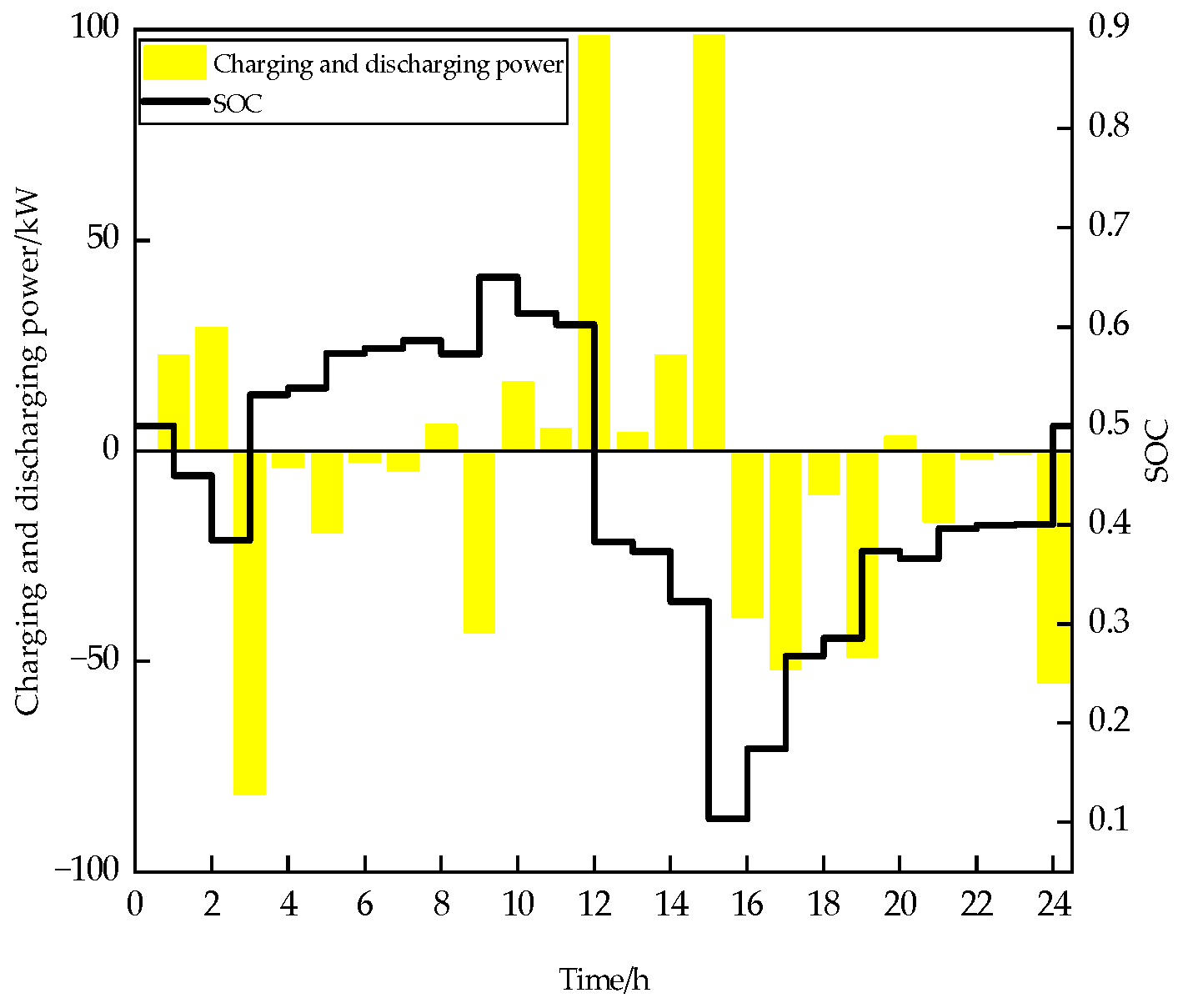
3.2. Demand-Side Energy Storage Model for Distribution Networks

Randomness in DG output and fluctuations in load demand force the distribution network to make higher requirements for stability and reliability. As a flexible resource with regulatory functions, energy storage has become an important component of ADN. From one perspective, it maintains the supply–demand balance of the system’s demand side, that is, when the power system is in a low load period, ESS stores electricity, and when it is in a high load period, they provide electricity, thereby achieving effective management and regulation of the power system’s load. From another perspective, it also supports increased utilization of renewable sources, reduces line losses, lowers transmission costs, and strengthens users’ adjustment and control of loads. In addition, the energy storage system requires frequent charging and discharging cycles during peak shaving and valley filling, but, inevitably, this will cause certain damage to the battery life. With the increase in system operating costs, accurate algorithms and reasonable control strategies are crucial to alleviate the two. Therefore, the H-WOA-GWO and on-site reactive power compensation strategy designed in research will play a guiding role in extending battery life and reducing grid costs.

The state of charge (SOC) of ESS represents the ratio between its remaining capacity and its total capacity at time t. The range of SOC values is generally from 10% to 90%. If the SOC is 0%, it signifies that ESS has been fully depleted; if the SOC is 100%, it signifies that ESS has reached full charge, and its state of charge equation is as follows [22]:

$$SO{C}_t={\displaystyle \frac{W_t}{W_{\mathrm{rate}}}}$$

(2)

where W_t represents the remaining capacity in the energy storage system at temporal point t; and W_rate denotes the total capacity in energy storage system.

To ensure the secure operation of ESS as well as to extend its service life, there is also a power limitation during its charging and discharging process, which is expressed as follows [23]:

$$P_{\mathrm{c}.\max }=\min \left\{P_{\mathrm{c}.\mathrm{rate}},{\displaystyle \frac{W_{\mathrm{ESS}}-W_{t-\Delta t}}{{\eta }_{\mathrm{c}}\Delta t}}\right\}$$

(3)

$$P_{\mathrm{d}.\max }=\min \left\{P_{\mathrm{d}.\mathrm{rate}},{\displaystyle \frac{(W_{t-\Delta t}-W_{\min }){\eta }_{\mathrm{d}}}{\Delta t}}\right\}$$

(4)

where P_c.max and P_d.max denote the maximum power levels for ESS charging and discharging operations, respectively; P_c.rate and P_d.rate, respectively, represent the rated charging and discharging power of ESS; W_ESS signifies capacity of ESS; W_t−Δt represents ESS capacity during t − Δt period; W_min indicates lower capacity limit for ESS; and η_c and η_d denote charging and discharging efficiencies for ESS, respectively.

3.3. Flexible Load Model Under Incentive-Based Demand Response

Flexible loads under an incentive-based demand response may be categorized as interruptible loads, curtailable loads, and shiftable loads based on their response characteristics and adjustment capabilities.

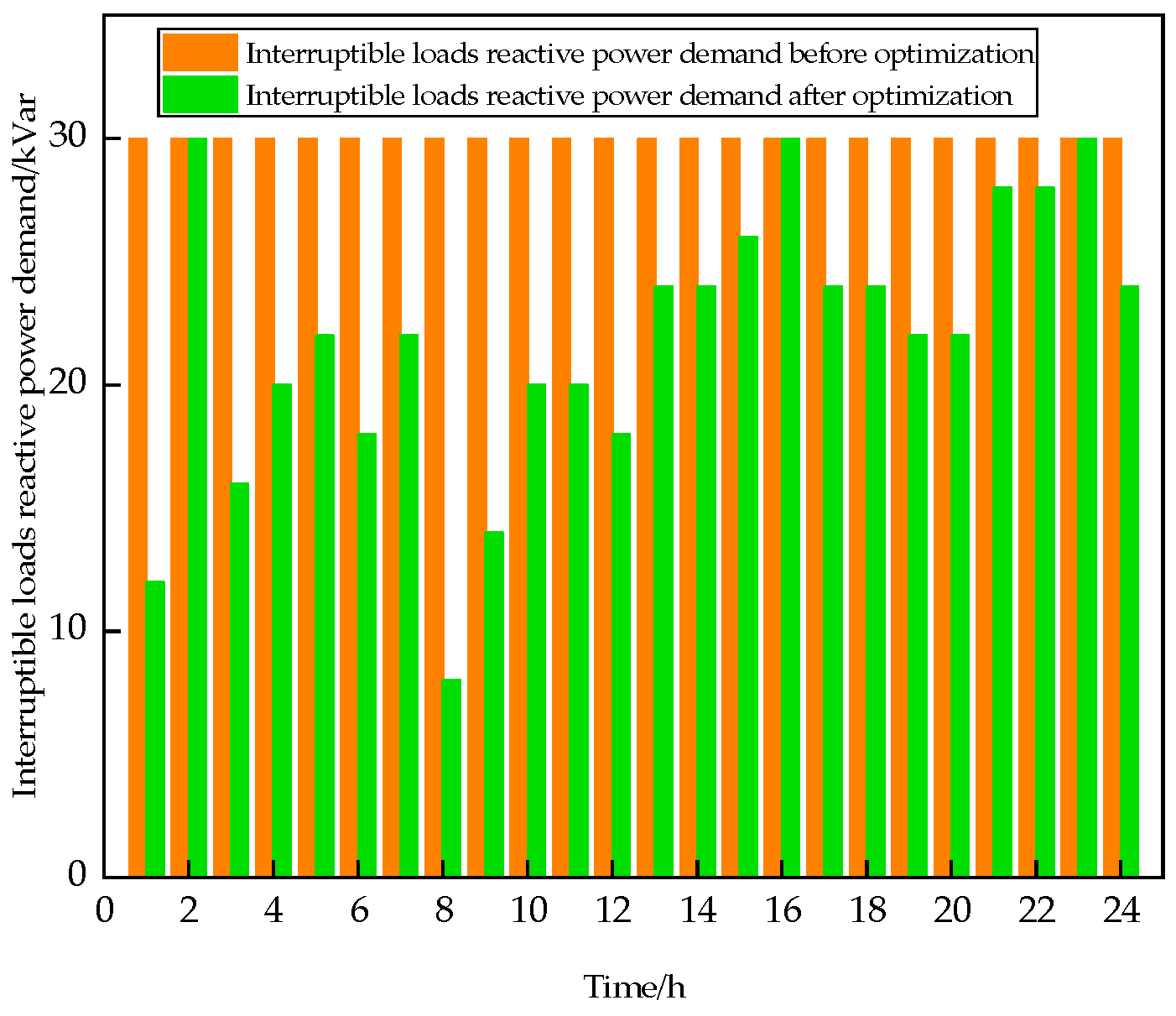
3.3.1. Interruptible Loads, IL

When the system load occurs during peak hours, intermittent start–stops of interruptible loads, represented by electric vehicles, can effectively alleviate peak load pressure on power grid. The start–stop constraint equation is as follows [24]:

$$x_{\mathrm{IL}.v}^t=\left\{\begin{array}{ll}1,\hfill & \mathrm{the}v\text{-}\mathrm{th}\mathrm{device}\mathrm{starts}\mathrm{up}\hfill \\ 0,\hfill & \mathrm{the}v\text{-}\mathrm{th}\mathrm{device}\mathrm{stops}\hfill \end{array}\right.$$

(5)

where $x_{\mathrm{IL}.v}^t$ represents the working state for the v-th interruptible load at temporal point t.

The equation for interruptible load reactive power output is as follows:

$$Q_{\mathrm{IL}.v}^t=P_{\mathrm{IL}.v}^t\tan {\phi }_{\mathrm{IL}.v}^t$$

(6)

where $P_{\mathrm{IL}.v}^t$ indicates active power for the v-th interruptible load at temporal point t; $Q_{\mathrm{IL}.v}^t$ represents reactive power demand for the v-th interruptible load at temporal point t; and ${\phi }_{\mathrm{IL}.v}^t$ indicates power factor angle for the v-th interruptible load at temporal point t.

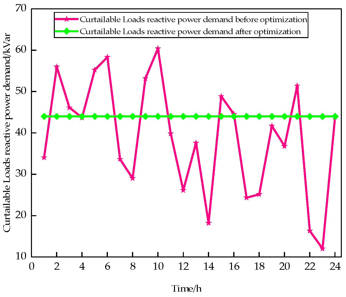
3.3.2. Curtailable Loads, CL

Taking air conditioning and HVAC equipment as an example, they have high power and great potential for load reduction. Such devices can be curtailable as needed during peak electricity consumption to sustain stable operation of the power grid. The equation for reactive power output is as follows:

$$Q_{\mathrm{CL}.m}^t=P_{\mathrm{CL}.m}^t\tan {\phi }_{\mathrm{CL}.m}^t$$

(7)

where $P_{\mathrm{CL}.m}^t$ indicates active power for the m-th curtailable load at temporal point t; $Q_{\mathrm{CL}.m}^t$ indicates reactive power demand for the m-th curtailable load at temporal point t; and ${\phi }_{\mathrm{CL}.m}^t$ indicates power factor angle for the m-th curtailable load at temporal point t.

The constraint equation for the curtailment amount of curtailable loads can be formulated as follows:

$$0⩽Q_{\mathrm{CL}.m}^t⩽Q_{\mathrm{CL}.m.\max }$$

(8)

where Q_CL.m.max indicates the maximum reactive power demand for the m-th curtailable load.

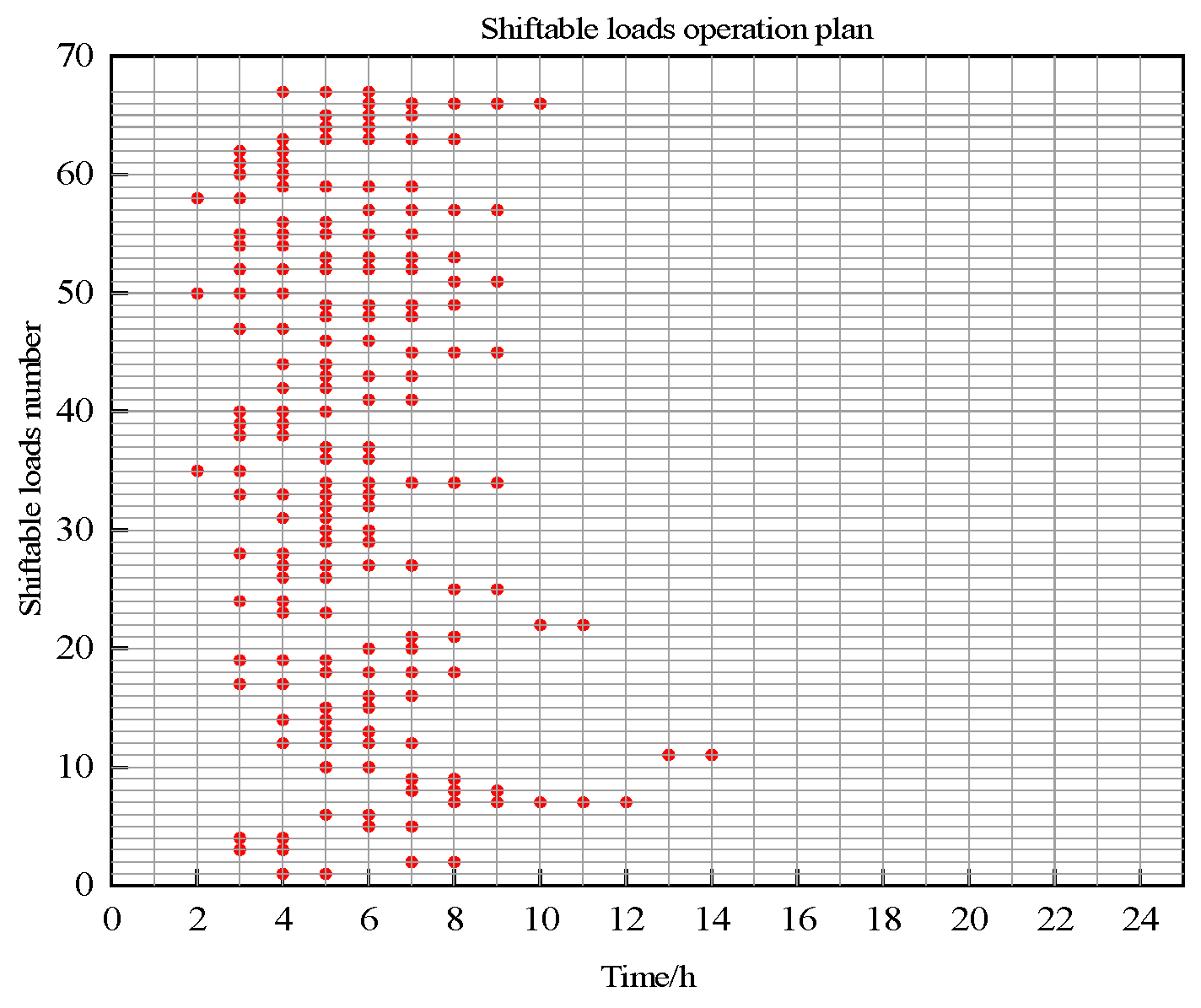
3.3.3. Shiftable Loads, SL

Shiftable loads can flexibly adjust their electricity consumption time within a specified time range. Taking household loads such as dryers and water heaters as examples, shiftable loads have power factor correction capabilities, so the power factor remains consistent before and after scheduling. The reactive power demand equation is as follows:

$$Q_{\mathrm{SL}.n}^t=P_{\mathrm{SL}.n}^t\tan {\phi }_{\mathrm{SL}.n}^t$$

(9)

where $P_{\mathrm{SL}.n}^t$ represents the active power for the n-th shiftable load at temporal point t; $Q_{\mathrm{SL}.n}^t$ indicates reactive power demand for the n-th shiftable load at temporal point t; and ${\phi }_{\mathrm{SL}.n}^t$ indicates power factor angle for the n-th shiftable load at temporal point t.

Shiftable loads, constrained by time windows, do not have a negative impact on users’ functional requirements and grid operation. Their equation is as follows:

$$\left\{\begin{array}{l}{Q}_{\mathrm{SL}.n}^{\mathrm{start}}=Q_{\mathrm{SL}.n}^{\mathrm{end}}\hfill \\ t_{\mathrm{SL}.n}^{\mathrm{start}}⩽t_{\mathrm{SL}.n}⩽t_{\mathrm{SL}.n}^{\mathrm{end}}-T_{\mathrm{SL}.n}\hfill \end{array}\right.$$

(10)

where $Q_{\mathrm{SL}.n}^{\mathrm{start}}$ and $Q_{\mathrm{SL}.n}^{\mathrm{end}}$ represent reactive power before and after transfer for the n-th shiftable load, respectively; $t_{\mathrm{SL}.n}^{\mathrm{start}}$ and $t_{\mathrm{SL}.n}^{\mathrm{end}}$ denote the allowable start and end time points for the n-th shiftable load within its time window constraint; t_SL.n signifies the starting point of the operational time for the n-th shiftable load after it responds; and T_SL.n indicates the continuous operational duration without interruption for the n-th shiftable load.

The electricity consumption demand of shiftable loads remains constant, with only the time period of consumption changing. Such loads exhibit significant regulation potential in demand response, peak shaving, and valley filling. These loads require continuous operation without interruption, and their operational state must satisfy the following constraints:

$$\left\{\begin{array}{l}{x}_{\mathrm{SL}.n}^t{x}_{\mathrm{SL}.n}^{t+1}\dots x_{\mathrm{SL}.n}^{t+u-1}=1\hfill \\ u=T_{\mathrm{SL}.n}/\Delta t\hfill \end{array}\right.$$

(11)

where $x_{\mathrm{SL}.n}^t$ indicates working state for the n-th shiftable load during time period t; u denotes number of regulation periods within operational time for the n-th shiftable load; and Δt signifies the scheduling time step.

4. Static Voltage Stability Index Under Active Distribution Network

4.1. Static Voltage Stability

With the diversification of load demand, the distribution network load also presents complex and diversified characteristics. Studying static voltage stability is conducive to further understanding the influence of load behavior regarding voltage stability, optimizing load management strategies, and enhancing ADN capability to adapt to large load fluctuations. Generally, the point of analysis is whether a voltage collapse will occur after a slow increase in load or small disturbances. From a mathematical perspective, static voltage stability essentially involves observing whether the equilibrium point of the PV curve or QV curve is in a stable region. The voltage of a network is usually supported by reactive power, and in severe cases of insufficient reactive power, the voltage cannot be maintained stably, resulting in instability.

The static voltage stability index can be categorized into the following main types: voltage margin index, voltage state index, etc. The voltage margin index (VSM) measures the system voltage stability margin by evaluating the gap between the present operating condition and the system collapse point. It finds the “nose tip point” by plotting the curve between the load power and voltage, and the disparity between the current load and point of collapse load is called the margin. The voltage state index (VSI) aims to assess the node voltage deviation extent from normal levels and predict the possible risk of voltage collapse based on this. The calculation of its index value is generally obtained through power flow calculation and sensitivity analysis [25].

4.2. Static Voltage Stability Index

The voltage stability index is often employed to evaluate the voltage stability of the network while quantifying the voltage stability status of a certain section of the line and node [26]. When facing complex power systems with multiple nodes, performing Thevenin equivalence at load node j can transform the complex power system into a simplified two nodes system. Figure 2 shows a simplified two nodes system.

The static voltage stability index Load_j is shown in the following equation [27,28]:

$$Loa{d}_j={\displaystyle \frac{4[V_i{V}_j\cos ({\delta }_i-{\delta }_j)-V_j^2{\cos }^2({\delta }_i-{\delta }_j)]}{V_i^2}}$$

(12)

where V_i, V_j are the voltage amplitudes at nodes; and δ_i, δ_j are the voltage phase angles at nodes.

The closer Load_j is to 0, the more stable the voltage state of line is; when the index approaches 1, it signifies that the system is tending towards instability and voltage collapse may occur. By calculating the Load_j index of all branches in ADN, the maximum Load_j index value is defined as the static voltage stability index of the entire ADN, which also symbolizes the characteristics of the weakest and most unstable branches in the system. The expression is shown in Equation (13):

$$Load=\max \left\{Loa{d}_1\right.,Loa{d}_2,\dots ,\left.Loa{d}_N\right\}$$

(13)

where N indicates number of branches in ADN.

5. Reactive Power Optimization Model

5.1. Optimization Variables

The reactive power $Q_{\mathrm{PV}.i}^t$ absorbed/emitted by the photovoltaic at bus i at temporal point t, the active power $P_{\mathrm{c}}^t$ and $P_{\mathrm{d}}^t$ charged/discharged by ESS at temporal point t, the working state $x_{\mathrm{IL}.v}^t$ for the v-th interruptible load at temporal point t, the reactive power $Q_{\mathrm{CL}.\mathrm{m}}^t$ for the m-th curtailable load at temporal point t, the working start time $t_{\mathrm{SL}.n}^{\mathrm{start}}$ and its sustainable working time $T_{\mathrm{SL}.n}$ for the n-th shiftable load, the number $u_{\mathrm{PCB}.i}^t$ of shunt capacitor banks (SCBs) put into operation at bus i at temporal point t, the tap position $u_{\mathrm{OLTC}}^t$ for on-load tap-changing transformer (OLTC) at time t, as well as the reactive power $Q_{\mathrm{STATCOM}}^t$ for static synchronous compensator (STATCOM) at time t.

5.2. Optimization Objectives

(1) Static voltage stability index. The static voltage stability index can effectively measure the system’s ability to resist collapse. With load dispatches or disturbances, this index can avoid power grid instability as much as possible, thereby ensuring its safe and stable operation. Therefore, it is set as one of the objective functions.

$$f_1=\min {\displaystyle \sum _{t=1}^{24}Loa{d}^t}$$

(14)

where Load^t is the static voltage stability index for ADN during time period t.

(2) Intraday nodal voltage deviation. The load and distributed generations in the active distribution network system of source–network–load–storage coordination have obvious temporal variation characteristics. Optimizing the node voltage deviation in the first 24 h of the day can effectively reduce such fluctuations, smooth the voltage changes in different time periods, and maintain a stable system during both peak and low load periods. Therefore, the 24 h voltage deviation is included in the optimization objective, and its expression is shown in Equation (15):

$$f_2=\min {\displaystyle \sum _{t=1}^{24}({\displaystyle \sum _{i=1}^{33}\left|U_i^t-1\right|})}$$

(15)

where $U_i^t$ indicates the voltage per unit value at bus i at temporal point t.

(3) Intraday network loss. Various flexible resources like DGs, ESSs, and flexible loads in active distribution networks affect the power flow and voltage distribution of power lines to a certain extent. By adjusting the charging and discharging behavior of ESS and utilizing peak shaving and valley filling to adjust load demand, the losses of lines can be greatly reduced. The equation for the current active power loss is as follows:

$$f_3=\min {\displaystyle \sum _{t=1}^{24}(U_i^t{\displaystyle \sum _{i,j\in 33}{G}_{ij}}(}{(U_i^t)}^2+{(U_j^t)}^2-2U_i^t{U}_j^t\cos {\theta }_{ij}^t))$$

(16)

where G is the conductivity; and ${\theta }_{ij}^t$ indicates phase difference of branch ij at time t.

(4) Punishment function. Given that the deviation range of the node voltage needs to be kept within ±5%, in order to encourage the algorithm to constrain it within a reasonable range, an additional penalty function is set, expressed as follows:

$$f_4=\min {\displaystyle \sum _{t=1}^{24}{\displaystyle \sum _{i=1}^{33}{\rho }_i}}{\left({\displaystyle \frac{\Delta U_i^t}{(U_{i.\max }-U_{i.\min })}}\right)}^2$$

(17)

where ρ_i is the penalty factor at node i; and U_i.max and U_i.min are set to 1.05 and 0.95, respectively.

To unify the dimensions, first, perform linear normalization on each sub-objective function, and finally convert it into a single objective function by assigning weights. Its equation is as follows:

$$F=\min \left({\omega }_1{F}_1+{\omega }_2{F}_2+{\omega }_3{F}_3+{\omega }_4{F}_4\right)$$

(18)

where F₁, F₂, F₃, and F₄ are the normalized values of each sub target, respectively; and ω₁, ω₂, ω₃, and ω₄ represent weights for each sub-objective, respectively. After simulation verification through numerical examples, it was found that taking ω₁ = ω₃ = 0.4 and ω₂ = ω₄ = 0.1 yields the best results.

5.3. Constraint Condition

Constraint on reactive power output for PV is as follows:

$$Q_{\mathrm{PV}.\min }^t<Q_{\mathrm{PV}.i}^t<Q_{\mathrm{PV}.\max }^t$$

(19)

Constraints for ESS are as follows:

$$\left\{\begin{array}{l}0.1⩽SO{C}_t⩽0.9\\ P_{\mathrm{c}.\min }⩽P_{\mathrm{c}}^t⩽P_{\mathrm{c}.\max }\\ P_{\mathrm{d}.\min }⩽P_{\mathrm{d}}^t⩽P_{\mathrm{d}.\max }\end{array}\right.$$

(20)

where P_c.min and P_d.min denote the minimum power levels for ESS charging and discharging operations, respectively.

Flexible load constraints are shown in Equations (5)–(11).

Given the inherent characteristics of shunt capacitor banks, the following constraints must also be met [29]:

$$\left\{\begin{array}{l}{Q}_{\mathrm{SCB}.i}^t=u_{\mathrm{SCB}.i}^t{Q}_{\mathrm{SCB}.\mathrm{rate}}\\ u_{\mathrm{SCB}.i}^t\in \{0,1,\cdots ,N_{\mathrm{SCB}}\}\end{array}\right.$$

(21)

where $Q_{\mathrm{SCB}.i}^t$ indicates the total reactive power generation from the shunt capacitor bank at bus i at temporal point t; Q_SCB.rate indicates the rated reactive power of a single capacitor; and N_SCB indicates the number of units assembled in shunt capacitor bank.

The amplitude of the primary side voltage for OLTC and its tap position must meet the following constraints [30]:

$$\left\{\begin{array}{l}{U}_{\mathrm{OLTC}.\mathrm{J}}^t=U_{\mathrm{OLTC}.\mathrm{S}}^t(1+u_{\mathrm{OLTC}}^{t}D)\\ u_{\mathrm{OLTC}}^t\in \{-N_{\mathrm{OLTC}},\cdots ,0,\cdots ,N_{\mathrm{OLTC}}\}\end{array}\right.$$

(22)

where $U_{\mathrm{OLTC}.\mathrm{J}}^t$ and $U_{\mathrm{OLTC}.\mathrm{S}}^t$ are the primary and secondary voltages for OLTC at temporal point t, respectively; D is the voltage difference among consecutive tap positions for OLTC; and N_OLTC is the gear position for OLTC.

The reactive power of a static synchronous compensator must meet following constraints [31]:

$$Q_{\mathrm{STATCOM}.\min }^t⩽Q_{\mathrm{STATCOM}}^t⩽Q_{\mathrm{STATCOM}.\max }^t$$

(23)

where $Q_{\mathrm{STATCOM}.\max }^t$ and $Q_{\mathrm{STATCOM}.\min }^t$ denote the upper and lower limits for static synchronous compensator at temporal point t, respectively.

The constraint equation for power flow balance is expressed as follows [32]:

$$\left\{\begin{array}{l}{P}_i^t=G_{ii}{\left(U_i^t\right)}^2+U_i^t{\displaystyle \sum _{j=1}^N}{U}_j^t(G_{ij}\cos {\theta }_{ij}^t+B_{ij}\sin {\theta }_{ij}^t)\\ Q_i^t=-B_{ii}{\left(U_i^t\right)}^2+U_i^t{\displaystyle \sum _{j=1}^N}{U}_j^t(G_{ij}\sin {\theta }_{ij}^t-B_{ij}\cos {\theta }_{ij}^t)\end{array}\right.$$

(24)

Among them:

$$P_i^t=P_{\mathrm{PV}.i}^T+P_{\mathrm{ESS}}^t-{\displaystyle \sum _{i=1}^{ILK}}{x}_{\mathrm{IL}.i}^t\frac{Q_{\mathrm{IL}.i}^t}{\tan {\phi }_{\mathrm{IL}.i}^t}-{\displaystyle \sum _{m=1}^{CLK}}\frac{Q_{\mathrm{CL}.m}^t}{\tan {\phi }_{\mathrm{CL}.m}^t}-{\displaystyle \sum _{n=1}^{SLK}}{x}_{\mathrm{SL}.n}^t\frac{Q_{\mathrm{SL}.n}^t}{\tan {\phi }_{\mathrm{SL}.n}^t}$$

(25)

$$Q_i^t=Q_{\mathrm{PV}.i}^T+Q_{\mathrm{PCB}.i}^t+Q_{\mathrm{STATCOM}}^t-{\displaystyle \sum _{i=1}^{ILK}}{x}_{\mathrm{IL}.i}^t{Q}_{\mathrm{IL}.i}^t-{\displaystyle \sum _{m=1}^{CLK}}{Q}_{\mathrm{CL}.m}^t-{\displaystyle \sum _{n=1}^{SLK}}{x}_{\mathrm{SL}.n}^t{Q}_{\mathrm{SL}.n}^t$$

(26)

where $P_{\mathrm{ESS}}^t$ represents the active power output from ESS at temporal point t; B is the susceptance between branches; ILk is the number of installed equipment with interruptible loads; CLk is the number of installed equipment with curtailable loads; and SLk is the number of installed equipment with shiftable loads.

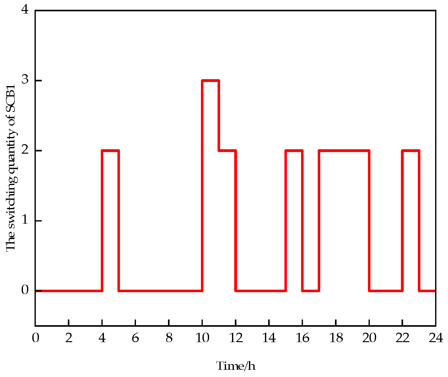
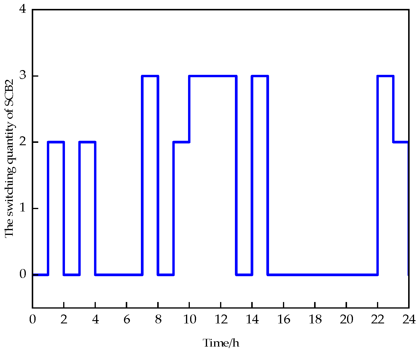
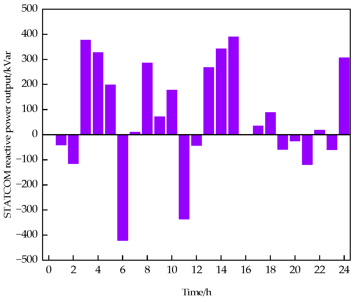
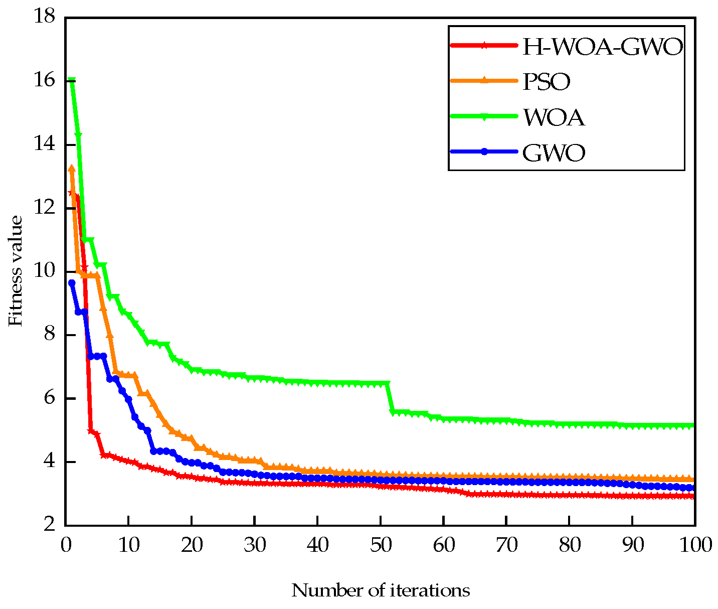
6. Case Studies and Analysis

The improved IEEE 33-bus DN, as shown in Figure 3, was used as the simulation experiment object while maintaining its line parameters unchanged. Node 14 and Node 33 were set as the grid-connection points for distributed generations DG1 and DG2, respectively. An energy storage system was installed at Node 6. SCBs were installed at Node 6 and Node 31 respectively, with N_SCB = 4, Q_SCB.rate = 150 kvar. OLTC was installed on branch 1–2, taking N_OLTC = 8, D = 0.0125. A STATCOM device was installed at Node 3, with $Q_{\mathrm{STATCOM}.\max }^t$ = 500 kvar, and $Q_{\mathrm{STATCOM}.\min }^t$ = −500 kvar. Interruptible loads were installed at Node 16. Curtailable loads were installed at Node 8. Shiftable loads were installed at Node 7. The collaborative interaction model is also effective in addressing communication latency and data synchronization challenges. The model can reduce communication latency to a certain extent and improve real-time data synchronization through the collaborative interaction of data between nodes.

The simulation analysis data selected in the article are the 24 h distributed photovoltaic active output and the IEEE 33 distribution network intraday load demand coefficient on a typical day. The curve variation is shown in Figure 4.

The various departments of the distribution network system achieve corresponding reactive power optimization strategies through data sharing and scheduling with each other, including the regulation of reactive power compensation devices and energy storage systems. Among them, STATCOM completes dynamic reactive power compensation by constructing self-commutation bridge circuits with switchable power electronic devices such as IGBT. Therefore, it is generally regarded as a continuous control variable, while the number of switching groups on the SCB and the tap position of the OLTC determine that it cannot continuously regulate reactive power output. Therefore, it is divided into discrete control variables. Considering the long response time and limited operating life of the SCB and OLTC, the control time interval is finally set to 1 h.

In the case of only considering the distributed grid-connection photovoltaic, the average static voltage stability index Load_j of all branches within 24 h was calculated using the MATPOWER 7.1 power flow calculation toolbox [33], as illustrated in

Table 1. Average static voltage stability index Load_j.

Line	Sending-End Bus	Terminal Bus	Loadj	Line	Sending-End Bus	Terminal Bus	Loadj
1	1	2	0.012769	17	17	18	0.003221
2	2	3	0.059920	18	2	19	0.002519
3	3	4	0.032175	19	19	20	0.016902
4	4	5	0.032135	20	20	21	0.003455
5	5	6	0.078774	21	21	22	0.003176
6	6	7	0.020878	22	3	23	0.016421
7	7	8	0.027288	23	23	24	0.031080
8	8	9	0.033033	24	24	25	0.015671
9	9	10	0.030902	25	6	26	0.006813
10	10	11	0.004488	26	26	27	0.008894
11	11	12	0.007929	27	27	28	0.036931
12	12	13	0.034187	28	28	29	0.026018
13	13	14	0.013688	29	29	30	0.011357
14	14	15	0.010880	30	30	31	0.018046
15	15	16	0.010922	31	31	32	0.003734
16	16	17	0.011822	32	32	33	0.000297

.

It is not difficult to see from Table 1 that the Load_j index of the fifth line is the highest, so its static voltage stability is the most vulnerable in the IEEE 33 node distribution network. Considering that ESS can not only peak load shifting and valley filling, enhance power supply reliability, but also effectively improve grid stability and reduce fluctuations and faults, the grid-connection point of ESS is set as the end node 6 of this branch, which greatly improves the overall static voltage stability. The simulation process adopts H-WOA-GWO for solving. The node voltages before and after optimization are shown in Figure 5 and Figure 6, and the average voltage values of each node prior to and following optimization are presented in Figure 7.

Through Figure 5, it was found that some nodes in the distribution network had voltage values below the lower limit before optimization, with the lowest value reaching 0.861015. At the same time, due to the high residential load level and lack of distributed photovoltaic output at night, the overall voltage level at that time was significantly lower than the normal level. However, with ESS and reactive power compensation device integration, the voltage amplitude for the distribution network system after source–network–load–storage joint planning was significantly improved, as shown in Figure 7.

The sum of active network losses, voltage deviations, static voltage stability indicators, and related penalty functions for the IEEE 33 node system within 24 h before and after various flexible resource collaborative interactions appear in

Table 2. Total 24 h data for ADN before and after collaborative interaction.

Optimization Objective	Before Collaborative Interaction	After Collaborative Interaction
Network loss	5.8216	5.0315
Voltage deviation	44.1509	20.6276
Static voltage stability index	1.8906	1.7060
Punishment function	6.3616	0

.

According to Table 2, compared to before the participation of various flexible resources in the interaction, network loss of the ADN decreased by 13.5719%. There has also been a significant improvement in voltage deviation, from 44.1509 before the interaction to 20.6276, which was 46.7207% before the interaction. Looking at Figure 7, it is found that the participation of various flexible resources and reactive power compensation devices is the main reason for the significant reduction in voltage deviation. The voltage fluctuation penalty function of the system before the interaction is still in a relatively dangerous range. However, the optimized system voltage will no longer exceed the limit, and voltage performance for ADN has been greatly enhanced. Finally, observations indicated that sum of the static index of the system decreased from 1.8906 to 1.7060, indicating that the interaction between various flexible resources and reactive power compensation devices further improved the static voltage stability of system.

The reactive power before and after the participation of various flexible resources is shown in Figure 8. In the former, photovoltaics only absorb reactive power, and after cooperating with other reactive power compensation devices, they will promptly supplement reactive power to ADN, greatly improving the overall voltage stability of system.

The charge–discharge cycle and state of charge of ESS within a 24 h period are shown in Figure 9, which plays multiple roles in improving the stability of ADN and flexibly adjusting active output throughout entire collaborative process.

The reactive power demand before and after the participation of multiple flexible loads in collaborative interaction is shown in Figure 10 and Figure 11.

The operation plan and reactive power demand after the participation of shiftable loads in collaborative interaction are shown in Figure 12 and Figure 13. The working period is mainly shifted to around 6:00. Therefore, from one perspective, peak reactive power demand is reduced by shifting the operation period, thus completing peak shaving and valley filling for the reactive power load curve. From another perspective, combined with Figure 10 and Figure 11, it is found that the overall reactive power demand is reduced after optimizing the multiple flexible loads, thereby reducing the reactive power flow on the branch and achieving the goal of reducing losses.

The switching process of shunt capacitor banks is shown in Figure 14 and Figure 15, where SCB1 outputs 300 kvar of reactive power during periods 4, 11, 15, 17–19, and 22, respectively. Only three sets of parallel capacitor units were switched during period 10. At the same time, SCB2 outputs 300 kvar of reactive power during periods 1, 3, 9, and 23. However, three sets of parallel capacitor units are also used during periods 7, 10–12, 14, and 22. It is not difficult to see that SCB significantly improves system stability through dynamic reactive power compensation.

Using ESS and reactive power compensation equipment to smooth out output power fluctuations of DG can reduce the regulation pressure of OLTC. In addition, when voltage fluctuates greatly, it is advisable to adopt a gradual adjustment method, observe for a period of time after each adjustment, and then decide whether to proceed with the next adjustment based on the actual situation. The process of changing the tap position of OLTC is shown in Figure 16. By introducing a transition circuit when switching the tap position, the current is limited to ensure a continuous current and regulation of the output voltage.

Considering that the system may experience transient instability when facing large disturbances such as sudden load changes, STATCOM can control the flow of reactive power by adjusting its output voltage and current, thereby improving the transient response of system, reducing system oscillation, accelerating voltage recovery, and enhancing system stability and reliability. The reactive power output for STATCOM is shown in Figure 17, which can achieve fast switching between inductive and capacitive reactive power, making STATCOM more suitable for situations that require fast, dynamic reactive power compensation, thereby improving power quality and reducing line losses.

The H-WOA-GWO designed in study can simultaneously integrate excellent local search capability of GWO and powerful global search capability of WOA, as well as ability to explore unknown areas. It also has significant advantages in handling different types of decision variables and solving dynamic reactive power optimization with a large and complex number of decision variables. The fitness value iteration curve is plotted as shown in Figure 18.

By combining the leader wolf mechanism of GWO, spiral update and contraction wrap mechanism of WOA, and speed update strategy of PSO, this multi strategy fusion helps balance global exploration and local exploitation in the search space, increasing the probability of the algorithm jumping out of local optima. Additionally, by introducing the strategy based on a covariance matrix and eigenvalue decomposition to capture distribution information of population, a statistical basis is provided for the adoption of GED strategy for high-quality solutions. As shown in Figure 18, H-WOA-GWO has faster convergence speed and higher convergence accuracy, as well as strong local development ability, making it less likely to fall into local optima.

7. Conclusions

This article mainly focuses on the voltage stability problem for ADN. By coordinating active and reactive power outputs of multiple flexible controllable resources, and introducing the Load_j index, a source–network–load–storage collaborative interaction model is formulated with the objectives of reducing intraday network loss, minimizing intraday voltage deviation, and optimizing static voltage stability. Based on this, optimization schemes for distributed photovoltaic, energy storage systems, multiple flexible loads, as well as reactive power compensation equipment are formulated. Finally, the following conclusions are drawn:

(1)

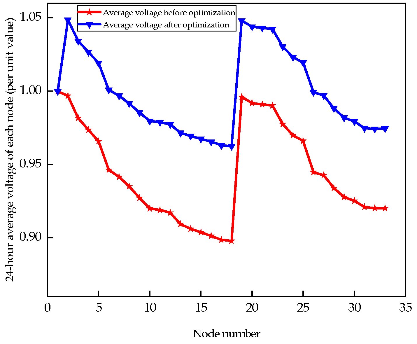
Simulation data shows that by coordinating distributed photovoltaics, energy storage, and multiple flexible loads to output each other, the voltage stability index of the network has been reduced by 9.7641% in comparison to the pre-optimization state, effectively improving the static voltage stability and voltage stability margin of network.

(2)

Intraday network loss of ADN has been reduced to 86.4281% of the original, and the overall voltage deviation has also been reduced to 46.7207% before optimization, effectively reducing operating costs and greatly avoiding the possibility of the voltage surpassing the threshold.

(3)

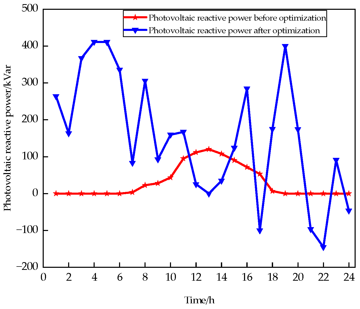
In the reactive power optimization model for ADNs incorporating collaborative interaction among sources, networks, loads, and storage, the voltage regulation capability is significantly enhanced through the classification of various types of flexible loads. This approach not only improves the network’s adaptability to intermittent fluctuations in renewable energy generation but also strengthens its overall responsiveness and operational efficiency.

The established source–network–load–storage collaborative interaction model contributes to the construction of smart cities, not only improving energy utilization efficiency to a certain extent, but also enhancing the stability of the power system, while providing strong support for the sustainable development of smart cities.

References

- Cui, Y.; An, N.; Fu, X.; Zhao, Y.; Zhong, W. Low-carbon economic dispatching of power system considering joint peak shaving of generalized energy storage and carbon capture equipment. Electr. Power Automat. Equip. 2023, 43, 40–48. [Google Scholar]
- Li, H.; Zhang, X.; Li, F.; Zhang, H.; Li, N.; Ma, X. Qinghai energy demand forecasting and development strategy research under the background of construction of clean energy demonstration province. Electr. Power. 2021, 54, 1–10+26. [Google Scholar]
- Yuan, J.H.; Zhang, H.N.; Zhang, J. Actively promoting power structure adjustment and accelerating the construction of a new power system. China Electr. Power Enterp. Manag. 2024, 13, 29–32. (In Chinese) [Google Scholar]
- Hou, H.; Chen, Y.; Liu, P.; Xie, C.; Huang, L.; Zhang, R. Multisource Energy Storage System Optimal Dispatch Among Electricity Hydrogen and Heat Networks From the Energy Storage Operator Prospect. IEEE Trans. Ind. Appl. 2022, 58, 2825–2835. [Google Scholar] [CrossRef]
- Wang, J.; Zhou, B.; Wang, T.; Lu, S. Design and implementation of decision support software for power grid planning with high proportion of renewable energy. Guangdong Electr. Power. 2021, 34, 50–59. [Google Scholar]
- Ai, H.; Wang, H. Distributionally robust optimization of load recovery for a multi-infeed HVDC receiving-end systems. Power Syst. Prot. Control. 2022, 50, 24–33. [Google Scholar]
- Zeng, G.; Ye, R.; Liu, W.; Huang, Y.; Li, J. The collaborative optimal dispatching of the medium voltage DC distribution network based on power flow calculation. Power Syst. Clean Energy. 2024, 40, 98–104. [Google Scholar]
- Wu, W.; Lin, C.; Sun, H.; Wang, B.; Liu, H.; Wu, G.; Li, P.; Sun, S.; Lu, J. Machine learning based energy management and operation control for active distribution networks. Autom. Electr. Power Syst. 2024, 48, 2–11. [Google Scholar]
- Zhou, L.; Zhou, Y.; Shen, W.; Huang, Z.; Li, L.; Li, Y. Reactive voltage optimization control of novel power system based on deep reinforcement learning. Electr. Meas. Instrum. 2024, 61, 182–189. [Google Scholar]
- Ai, Y.; Du, M.; Pan, Z.; Li, G. The optimization of reactive power for distribution network with PV generation based on NSGA-III. CPSS Trans. Power Electron. Appl. 2021, 6, 193–200. [Google Scholar] [CrossRef]
- Ren, Y.; Song, J.; Yu, R.; Wang, W.; Xing, B.; Wu, J. Coordinated optimization of reactive power compensation device in distribution network considering on demand-side response. Smart Power. 2024, 52, 79–86. [Google Scholar]
- Chen, Q.; Wang, W.; Wang, H.; Wu, J. Research on dynamic reactive power compensation optimization strategy of distribution network with distributed generation. Acta Energ. Sol. Sin. 2023, 44, 525–535. [Google Scholar]
- Sun, R.; Yuan, Z.; Wang, W.; He, S. Multi-objective optimization of dynamic reactive power in a new distribution network with a solid state transformer. Power Syst. Prot. Control. 2023, 51, 104–114. [Google Scholar]
- Qiao, L.; Wang, T.; Liu, J.; Li, X.; Wu, C. Distribution network reactive power optimization considering generation network load storage interaction. Electr. Meas. Instrum. 2024, 61, 146–151+189. [Google Scholar]
- Liu, Y.; Huang, M.; Zhang, Y.; Zhang, L.; Liu, W.; Yu, H.; Wang, F.; Li, L. Coordinated Optimization Method of Electric Buses and Voltage Source Converters for Improving the Absorption Capacity of New Energy Sources and Loads in Distribution Networks. Energies 2025, 18, 832. [Google Scholar] [CrossRef]
- Chen, Y.; Ma, X.; Cheng, K.; Bao, T.; Chen, Y.; Zhou, C. Ultra-short-term power forecast of new energy based on meteorological feature selection and SVM model parameter optimization. Acta Energ. Sol. Sin. 2023, 44, 568–576. [Google Scholar]
- Phan, T.M.; Duong, M.P.; Doan, A.T.; Duong, M.Q.; Nguyen, T.T. Optimal Design and Operation of Wind Turbines in Radial Distribution Power Grids for Power Loss Minimization. Appl. Sci. 2024, 14, 1462. [Google Scholar] [CrossRef]
- Ma, X.; Li, Y.; Liang, C.; Dong, X.; Xu, R. Reactive power optimization for loss reduction of distribution network considering interactions of high penetration level of multiple regulating energy resources. Electr. Power 2024, 57, 123–132. [Google Scholar]
- Zhang, Y.; Chen, J.; Guo, L.; Shen, J.; Zhai, W.; Dong, H.; Zhang, J.; Fang, R. Research on dynamic reactive power optimization method of active distribution network considering flexible and controllable resources. Electr. Automat. 2023, 45, 30–33. [Google Scholar]
- Lei, C.; Bu, S.; Chen, Q.; Wang, Q.; Wang, Q.; Srinivasan, D. Decentralized Optimal Power Flow for Multi-Agent Active Distribution Networks: A Differentially Private Consensus ADMM Algorithm. IEEE Trans. Smart Grid. 2024, 15, 6175–6178. [Google Scholar] [CrossRef]
- Zhang, X.; Xu, Y.; Xu, S.; Xiao, X. Fundamental Approximation Model and Frequency Characteristics of CPS-PWM with Asymmetric Regular Sampling. Autom. Electr. Power Syst. 2020, 44, 91–97. [Google Scholar]
- Mitra, S.K.; Karanki, S.B. An SOC Based Adaptive Energy Management System for Hybrid Energy Storage System Integration to DC Grid. IEEE Trans. Ind. Appl. 2023, 59, 1152–1161. [Google Scholar] [CrossRef]
- Xiao, Y.; Xiao, X.; Jin, X.; He, X.; Feng, J.; He, X. Multi-objective optimization of distribution network system with energy storage and distributed photovoltaic considering static voltage stability. Guangdong Electr. Power 2024, 37, 24–32. [Google Scholar]
- Dehghani, M.; Bornapour, S.M.; Sheybani, E. Enhanced Energy Management System in Smart Homes Considering Economic, Technical, and Environmental Aspects: A Novel Modification-Based Grey Wolf Optimizer. Energies 2025, 18, 1071. [Google Scholar] [CrossRef]
- Wang, G.; Xin, H.; Wu, D.; Li, Z.; Ju, P. Grid Strength Assessment for Inhomogeneous Multi-infeed HVDC Systems via Generalized Short Circuit Ratio. J. Mod. Power Syst. Clean Energy 2023, 11, 1370–1374. [Google Scholar] [CrossRef]
- Xu, J.; Lan, T.; Liao, S.; Sun, Y.; Ke, D.; Li, X. An on-line power/voltage stability index for multi-infeed HVDC systems. J. Mod. Power Syst. Clean Energy 2019, 7, 1094–1104. [Google Scholar] [CrossRef]
- Makasa, K.J.; Venayagamoorthy, G.K. Venayagamoorthy. Estimation of voltage stability index in a power system with Plug-in Electric Vehicles. In Proceedings of the 2010 IREP Symposium Bulk Power System Dynamics and Control-VIII (IREP), Rio de Janeiro, Brazil, 1–6 August 2010. [Google Scholar]
- Li, S.; Gao, Y.; Jiang, C. A static voltage stability index based on PV curve for the medium-voltage distribution network with distributed PV. J. Phys. Conf. Ser. 2023, 2591, 12042. [Google Scholar] [CrossRef]
- Wang, H.; Li, C.; Zhu, G.; Liu, Y.; Wang, H. Model-Based Design and Optimization of Hybrid DC-Link Capacitor Banks. IEEE Trans. Power Electron. 2020, 35, 8910–8925. [Google Scholar] [CrossRef]
- Jafari, M.R.; Parniani, M.; Ravanji, M.H. Decentralized Control of OLTC and PV Inverters for Voltage Regulation in Radial Distribution Networks With High PV Penetration. IEEE Trans. Power Del. 2022, 37, 4827–4837. [Google Scholar] [CrossRef]
- Sonawane, A.J.; Umarikar, A.C. Voltage and Reactive Power Regulation With Synchronverter-Based Control of PV-STATCOM. IEEE Access 2023, 11, 52129–52140. [Google Scholar] [CrossRef]
- Li, P.; Wu, W.; Wang, X.; Xu, B. A Data-Driven Linear Optimal Power Flow Model for Distribution Networks. IEEE Trans. Power Syst. 2023, 38, 956–959. [Google Scholar] [CrossRef]
- Zimmerman, R.D.; Murillo-Sánchez, C.E.; Thomas, R.J. MATPOWER: Steady-State Operations, Planning, and Analysis Tools for Power Systems Research and Education. IEEE Trans. Power Syst. 2011, 26, 12–19. [Google Scholar] [CrossRef]