Abstract
Traditional clustering methods are often ineffective in extracting relevant features from high-dimensional, nonlinear near-infrared (NIR) spectra, resulting in poor accuracy of detecting lactose-free milk adulteration. In this paper, we introduce a clustering model based on Gram angular field and convolutional depth manifold (GAF-ConvDuc). The Gram angular field accentuates variations in spectral absorption peaks, while convolution depth manifold clustering captures local features between adjacent wavelengths, reducing the influence of noise and enhancing clustering accuracy. Experiments were performed on samples from 2250 milk spectra using the GAF-ConvDuc model. Compared to K-means, the silhouette coefficient (SC) increased from 0.109 to 0.571, standardized mutual information index (NMI) increased from 0.696 to 0.921, the Adjusted Randindex (ARI) increased from 0.543 to 0.836, and accuracy (ACC) increased from 67.2% to 88.9%. Experimental results indicate that our method is superior to K-means, Variational Autoencoder (VAE) clustering, and other approaches. Without requiring pre-labeled data, the model achieves higher inter-cluster separation and more distinct clustering boundaries. These findings offer a robust solution for detecting lactose-free milk adulteration, crucial for food safety oversight.
1. Introduction
Lactose intolerant individuals may experience digestive discomfort and health issues if they consume lactose. Traditional methods for detecting milk adulteration adopt reagent-based approaches, such as enzyme-linked immunosorbent assay (ELISA) [1], which can damage the sample and are costly and inefficient. It is difficult to detect low concentration adulterated substances. High-performance liquid chromatography (HPLC) [2] is a separation method with high sensitive, but it is costly, complex to operate, and has a long detection time. Therefore, it is necessary to research and develop a rapid, non-destructive, and highly sensitive method for detecting milk adulteration.
In recent years, molecular biology methods and optical sensor methods have achieved some results in the detection of milk adulteration. Tsakali et al. [3] proposed the polymerase chain reaction (PCR) method for detecting cow’s milk adulteration in 40 goat milk products. Harini et al. [4] developed a fiber optic sensor based on the lossy mode resonance method, which can detect formaldehyde and water adulteration in three types of milk. Although the costs of these two methods have decreased, they require high laboratory standards, or different types of adulterants require different sensor strategies, which increase the complexity of their technical applications.
With the development of computer application technology, there is a growing trend in milk adulteration detection to integrate physicochemical analytical techniques with chemometrics, especially near-infrared spectroscopy (NIR) analysis techniques. NIR analysis technology has the advantages of non-destructive testing, high detection efficiency, and simultaneous analysis of multiple components. At present, this detection method can be divided into three types as follows: statistical methods, machine learning methods, and deep learning methods. Statistical methods mainly include principal component analysis (PCA), partial least squares regression (PLS), and linear discriminant analysis (LDA). Feng et al. [5] selected the 4000–400 cm−1 wavenumber range as variables to perform PCA on the obtained spectral data, identifying five categories of milk. Huang et al. [6] used near-infrared spectroscopy combined with PLS to quickly determine the urea content adulterated in milk. Wei et al. [7] used PCA, LDA, and PLS to perform discriminant analysis on the NIR data of pure milk and milk adulterated with melamine at different concentrations. These methods are simple and fast, but the generalization ability of the models is limited, sensitive to outliers, and the model performance decreases when dealing with nonlinear relationships.
Machine learning methods mainly include decision tree (DT), support vector machine (SVM), and random forest (RF). Currently, it is common to combine statistical methods and machine learning methods for milk adulteration detection to improve the accuracy and reliability of detection. Farah [8] used differential scanning calorimetry combined with machine learning methods to detect adulterants such as formaldehyde, whey, and urea in raw milk. The RF model performed the best. Cai et al. [9] used a data-driven soft independent classification model (DD-SIMCA) to classify camel milk powder samples, and employed the RF algorithm to improve classification accuracy, which could distinguish between different types of adulteration in camel milk powder. Wu et al. [10] proposed the FiNLDA method, which extracts features from milk near-infrared spectral data and combines them with a K-nearest neighbor classifier, effectively classifying milk brands better than LDA and iNLDA. Yu et al. [11] proposed a new method for near-infrared spectral feature extraction, using GADF to convert one-dimensional spectra into two-dimensional images. A multi-scale CNN model containing an Inception structure was constructed to discriminate pesticide types, and good discrimination performance was obtained.
Deep learning methods mainly include convolutional neural networks (CNNs), recurrent neural networks (RNNs), and autoencoders. Traditional statistical and machine learning methods perform well when dealing with modeling problems with moderate data volumes and appropriate feature selection, but they perform poorly when faced with large data volumes and complex features. Deep learning excels at automatically learning features from datasets. Neto et al. [12] used CNN to directly analyze the Fourier transform infrared (FTIR) spectra of adulterated milk without preprocessing, identifying more effectively than traditional methods. Chu et al. [13] improved the accuracy of milk adulteration detection by combining FTIR spectroscopy with machine learning algorithms, including multi-layer perceptron (MLP), bayesian regularized neural network (BRNN), extreme gradient boosting (XGB), and projection pursuit regression (PPR) algorithms. Similar studies have been conducted in other quality detection applications. Rashvand [14] used hyperspectral imaging (HSI) technology to evaluate carbohydrate content. They developed partial least squares regression (PLSR), SVM regression, and temporal convolutional network attention (TCNA) to estimate the carbohydrate content in soy flour. Ninh et al. [15] employed NIR spectroscopy technology to evaluate fish quality by measuring histamine levels, collecting spectral data from 284 fish samples across eight distinct body sites. They developed machine learning models, including DT, K-Nearest Neighbors (KNNs), SVM, and XGB, as well as CNNs. The experimental results indicated that the CNN model outperformed traditional machine learning in evaluating fish quality.
However, the above methods employ supervised learning approaches, which are highly dependent on labeled data and have poor recognition capabilities for unknown adulterated samples. It is difficult and costly to obtain a large number of adulterated samples in practical applications. Therefore, in order to solve the above problems, one might consider studying unsupervised learning methods for milk adulteration detection. Zain et al. [16] used PCA and hierarchical cluster analysis to study 24 essential and trace elements in 231 samples of raw and factory milk. They found that eight trace elements were discriminative factors for separating Malaysian milk samples from those of some other regions worldwide. Crase et al. [17] investigated the latest progress in clustering analysis of infrared and NIR spectral data. According to the characteristics of high-dimensional and low-sample spectral data, they pointed out the shortcomings of quantitative analysis and evaluation in current practice. The clustering analysis model and workflow suitable for NIR spectral data were proposed. Buoio et al. [18] proposed a method based on a portable FTIR spectrometer and a VC-SVM hybrid model. By using variable clustering for data preprocessing and feature selection, the performance of the SVM model was optimized to achieve rapid identification of milk with different fat contents. Guan et al. [19] used PCA to reduce the dimension of the spectral data for each sample, followed by analysis of 11 types of soil from different regions using the K-means clustering algorithm. The clustering after dimensionality reduction can reduce the impact of outliers on clustering performance. All these show that traditional clustering algorithms can classify samples with similar spectral features into one class, revealing the inherent structure of the data itself. However, since traditional clustering algorithms rely on distance metrics to evaluate the similarity between points, they encounter the “curse of dimensionality” problem in high-dimensional spaces, so the clustering performance is difficult to improve.
Compared with traditional clustering, deep clustering methods have the powerful feature extraction ability of deep learning and data grouping ability of clustering algorithms. At present, deep clustering methods have been widely applied in image recognition and bioinformatics, but their application in NIR spectral analysis has not yet been seen. Deep clustering methods mainly include the autoencoder (AE) [20], variational autoencoder (VAE) [21], and deep embedding clustering (DEC) [22]. These methods can find complex data structures that are difficult for traditional clustering methods to capture. They perform better when handling high-dimensional data. Jo et al. [23] studied the geographical source discrimination methods of eight different agricultural products. Using AE for the feature extraction of near-infrared spectra can improve the SVM classification accuracy for the geographical traceability of agricultural products, which is better than the direct use of the original spectrum. However, this method fails to achieve end-to-end learning and increases the computational complexity and time cost. The autoencoder only plays a role in reconstructing the input data, rather than obtaining features optimized for the classification task. The deep embedded clustering method calculates similarity based on the Euclidean distance between data points and cluster centers. The method is sensitive to the choice of initial centers. If there is a lot of noise in the input data, it will reduce clustering performance, and some clustering boundaries will be blurred.
In summary, the deep clustering method is applied to NIR spectral analysis, which can reduce the reliance on labeled data, decrease modeling costs, and improve the recognition ability of unknown class samples. Due to the presence of noise in the NIR spectra of milk, the severe overlap of absorption peaks and peak shapes is wide. The spectral features of low-concentration adulterants are easily obscured by the strong absorption peaks of the main components of milk. Therefore, we introduces the Gram angular field method to enhance the ability of the convolutional encoder to extract detailed features, and we combine it with deep manifold clustering to propose a hybrid model named GAF-ConvDuc.
The remaining part of this article is organized as follows: Section 2 introduces the related work of feature imageization and deep clustering. Section 3 describes in detail the principle of the GAF-ConvDuc algorithm, network structure, and model evaluation indicators. Section 4 provides the experimental results, conducting in-depth analysis from multiple perspectives such as parameter influence, ablation experiments, and model comparison to verify the validity of the model. Finally, the work is concluded in Section 5.
2. Related Work
2.1. Feature Imageization
The feature imageization method is used to transform the features of high-dimensional data into images through visualization techniques. Common methods include principal component analysis projection plots, heat maps, wavelet plots, spectrograms, recurrence plots, GAF, and the Markov transition field (MTF). In fields such as fault detection, behavior recognition, biometric signal processing, and climate change analysis, time series visualization methods are being gradually more widely applied. Hu et al. [24] proposed a gear fault classification method based on root strain and pseudo-images. The method involves preprocessing the strain signals, converting them into 2D images, and extracting features using CNN-EfficientNet, with excellent performance in experiments. Lei et al. [25] proposed a method for diagnosing rolling bearing faults based on MTF and a pyramid cascaded multi-dimensional CNN model. MTF converts one-dimensional vibration signals into two-dimensional images, and CNN extracts fault information from these feature maps, improving the diagnostic accuracy and versatility of rolling bearing diagnosis.
Feature visualization methods are gradually being applied in NIR spectral analysis as well. Zhao et al. [26] proposed a method to distinguish between normal and watercored apples, combining GAF encoding and the ConvNeXt model, using near-infrared spectroscopy. By converting spectral data into two-dimensional images and inputting them into the ConvNeXt model, deep feature information can be extracted, thereby improving classification accuracy. Liu et al. [27] proposed a data fusion modeling method based on NIR spectral imaging. After preprocessing the reflectance spectra using continuous wavelet transform (CWT), the one-dimensional spectra are converted into Gramian angular difference field and Gramian angular sum field images through GAF encoding, and fused images are generated. The ViT-2D/1D-CNN-DF model extracts features from the GADF images preprocessed by CWT, significantly improving the model’s accuracy.
The above-mentioned study demonstrates that feature visualization methods, by converting one-dimensional signals into two-dimensional images, can intuitively display the spatiotemporal changes of data and extract subtle variations that were previously difficult to detect, thereby enhancing the features for fault signal detection and item classification. Therefore, this paper introduces the feature visualization method of Gramian Angular Fields to enhance the features of milk near-infrared spectra, providing effective features for convolutional autoencoders, and thus improving the clustering performance of deep clustering models.
2.2. Autoencoder
Autoencoders are primarily utilized for unsupervised learning and data dimensionality reduction, comprising encoders and decoders. The encoder learns to compress input data into a low-dimensional representation, while the decoder reconstructs the original input from this representation. Autoencoders primarily include variational autoencoders, denoising autoencoders, sparse autoencoders, and convolutional autoencoders. Deng et al. [28] utilized a one-dimensional convolutional autoencoder (1D-CAE) to compress spectral data. The compressed features were integrated with SVM and PLS models to develop an evaluation model for the antioxidant level of edible oil. Zhuang et al. [29], in view of the limitations of the traditional dimensionality reduction methods in near-infrared spectroscopy, applied the contrastive variational autoencoder to the detection of melamine adulteration in milk, achieving the decoupling of nonlinear features and parametry-free adaptive separation. Du et al. [30] designed CAE for spectral feature extraction and classification, which includes an encoding, decoding, and classification network. In the experiment on classifying hot jet streams of an aero-engine, the CAE demonstrated higher precision and efficiency, outperforming PCA and various classic classifiers, as well as other deep learning methods. Yang et al. [31] proposed the two-stage model TMC-SAE, which combines the two sub-models, SAE-1 and SAE-2. SAE-1 is based on fully connected layers and one-dimensional convolutional autoencoders and is used to reduce the spectral dimension. SAE-2 is a hybrid autoencoder composed of 2D and 3D convolution operations, which is used to extract spectral–spatial features and improve the classification accuracy of hyperspectral images.
In this paper, in order to capture the spatial hierarchical structure in GAF images and demonstrate higher accuracy and efficiency in reconstructing GAF images, we will use a convolutional autoencoder as the pre-training and embedding module for deep clustering. During the encoding and decoding processes, convolutional operations are used to better extract the local features of the GAF image.
2.3. Deep Embedded Clustering Framework
Deep embedded clustering algorithms address the limitations of traditional clustering methods in handling high-dimensional, complex data. They are currently mainly applied in image segmentation, object recognition, and lesion identification tasks in the medical field. Deep embedded clustering can learn low-dimensional embedded representations of data, capture nonlinear structures and complex patterns, and perform more effective clustering in the embedded space. Mengli L et al. [32] proposed a deep embedded clustering algorithm based on a residual autoencoder (DECRA). By introducing an adaptive weighting layer in the feature representation, it can achieve good robustness, accomplish generalization for specific tasks, and adaptively learn better feature embeddings based on classification. Bai et al. [33] proposed a DEC method for clustering load curves and extracting representative patterns. This method involves the feature extraction of user electricity load data using one-dimensional convolutional autoencoders, followed by optimization through low-dimensional embedding clustering. Compared with K-means and IDEC methods, the clustering performance index has been significantly improved. Duan et al. [34] proposed a method for clustering image and text data using deep embedding, cluster estimation, and metric learning. Low-dimensional representations are generated through a deep autoencoder, the number of clusters is estimated using a softmax autoencoder, and a distance metric is learned via a Siamese network to enhance clustering performance.
Feng [35] proposes a dimensionality reduction method using Variational Autoencoder Uniform Manifold Approximation and Projection to address the crowding problem in existing dimensionality reduction methods. First, the data are compressed into latent variables using a Variational Autoencoder and then further reduced through Uniform Manifold Approximation and Projection, maintaining the similarity of the data. Nie [36] addressed the detection accuracy issue of YOLOv5 by proposing an improved model based on multi-task loss optimization. This model enhances the accuracy of position and classification by applying clustering adaptive loss weight allocation to the predicted bounding boxes of the same target across feature maps of different resolutions.
Due to the random initialization of the initial cluster centers in deep embedded clustering, the algorithm is prone to getting stuck in local optima, which reduces clustering performance. Therefore, it is necessary to consider robust initialization methods, combined with the K-means++ algorithm to select the initial center points, improving the quality of the initial clustering.
In summary, VAE clustering may result in an over-smoothing latent space, causing cluster boundaries to become blurred. When the model structure and parameter selection are inappropriate, convolutional autoencoders (CAE) can lead to inadequate feature representation or overfitting. In this paper, considering that deep embedded clustering has advantages in automatic feature extraction and identifying unknown classes and robustness, we replace the feedforward neural network autoencoder with a CAE to more effectively capture local features in GAF images and remove noise and redundant data. The uniform manifold approximation is introduced into the clustering module to improve the quality and distribution of the clustering centers. The adaptive boundary loss function is introduced into the loss function to reduce the ambiguity on the clustering boundary, increase the degree of separation between classes, and improve the generalization ability of clustering.
3. Method
3.1. Gramian Angular Fields
The GAF method pairs data points from a sequence, computing the cosine of the angles between them and converting these results into pixel intensities within an image [37,38]. Original NIR data are represented as , where is the absorbance at the i-th wavelength. By applying min–max normalization to scale the series S to the range [−1, 1], a new sequence is obtained, as shown in Equation (1):
The arccosine of the normalized near-infrared spectra is calculated using in polar coordinates, defined in Equation (2), expressed as follows:
GAF consists of summation fields (GASFs) and difference fields (GADFs). By employing cosine functions, these fields calculate the sum or difference of angles, respectively, resulting in the generation of the Gramian matrix. The calculation of GASF appears in Equation (3) as follows:
Finally, the matrix values are mapped to the pixel values of an image for imageization. The image data serve as the input to the convolutional autoencoder.
3.2. Convolution Embedding Manifold Clustering
3.2.1. Convolution Autoencoder
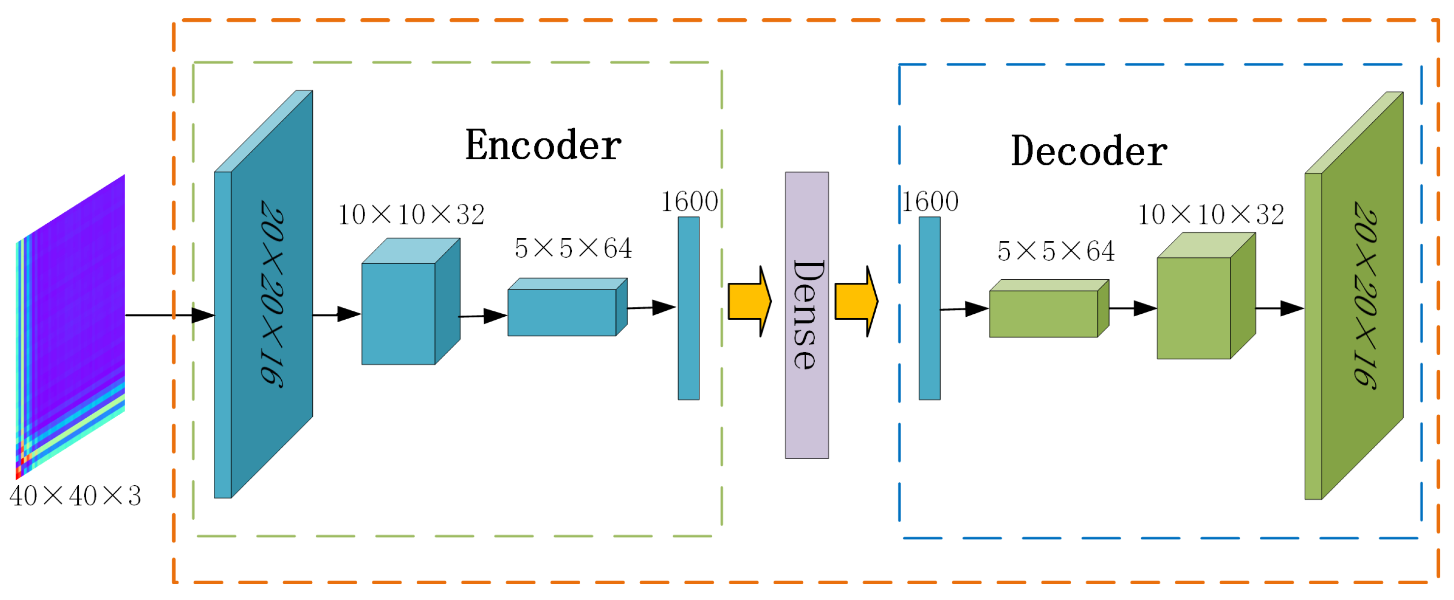
Autoencoders [39] are unsupervised neural network models used for tasks such as dimensionality reduction, feature extraction, and data reconstruction. Compared to feedforward neural networks, the convolutional autoencoders are more capable of extracting features from images generated by GAF. As shown in Figure 1, in this paper, the convolutional autoencoder consists of two parts. The encoder consists of three convolutional layers that transform the input image to low-dimensional feature vectors, along with a flattening layer. The decoder consists of three transposed convolutional layers, which reconstruct the latent representation back to the original image, also incorporating a flattening layer. The reconstruction loss function is defined as in Equation (4), expressed as follows:
where denotes the i-th image, represents the encoder function, and represents the decoder function. The autoencoder is trained by minimizing this reconstruction loss. During the pre-training phase, the low-dimensional embedding representations of all image samples are obtained through the convolutional autoencoder, denoted as .

Figure 1.
Architecture of the convolutional autoencoder.
3.2.2. Integrating Uniform Manifold Clustering
During the fine-tuning phase, deep clustering comprises three main steps as follows: initializing cluster centers, calculating soft assignments and target distributions, and iteratively optimizing the encoder parameters and cluster centers.
Due to its sensitivity to noise and parameter k, K-means clustering often falls into local optima and fails to handle clusters with uneven density distributions effectively. To overcome these issues, we introduce uniform manifold approximation for dimensionality reduction before K-means clustering, improving the selection of initial cluster centers.
Uniform manifold approximation [40,41] can map high-dimensional data while retaining the original structure of the data. It involves calculating the Euclidean distance matrix D, identifying the nearest neighbors for each data point, and constructing a weighted graph in the high-dimensional space. The objective function minimizes the cross-entropy between the probability distributions in the high-dimensional and low-dimensional spaces, defined as in Equation (5), as follows:
where and , respectively, represent the similarity probabilities between the data before and after mapping.
Our algorithm incorporates uniform manifold approximation for mapping high-dimensional data to a low-dimensional space. Initial cluster centers are derived using the K-means++ algorithm [42] on dimension-reduced data. Subsequently, the algorithm computes soft assignments Q between data points and cluster centers, optimizes the target distribution P, and iteratively minimizes the KL divergence [43,44,45] between P and Q to form the clustering loss. This process is detailed in Equations (6)–(8), as follows:
Here, represents the j-th centroid, and denotes the degrees of freedom parameter.
Following numerous learning iterations, each data point is assigned to the cluster center with the highest probability, yielding the final clustering output .
3.2.3. Improved Adaptive Margin Loss
Some sample points have features that are similar to multiple clusters, and their clustering results are located at the boundaries of multiple clusters, rendering them prone to misclassification. Additionally, noise points can also cause the clustering boundary areas to become more blurred. In order to solve this problem, on the basis of reconstruction loss and clustering loss, the total loss function has been improved by adding an adaptive margin loss [46]. The adaptive margin loss dynamically adjusts boundaries between data points, better distinguishing the clusters to which samples belong during the training process.
Let the low-dimensional embedding feature vector be . Adaptive margin loss consists of intra-cluster loss, inter-cluster loss, and boundary loss, defined as in Equation (9), as follows:
where is the number of sample pairs within cluster C and is the number of sample pairs between different clusters. is the initial boundary threshold (initial value = 0.5), is the adjustment factor, and and represent the average distances between samples of the same and different clusters, respectively. The indicator variable equals 1 when two samples are in the same cluster and −1 otherwise. The variable represents the distance between these samples.
The total loss is defined as the sum of reconstruction loss, adaptive margin loss, and clustering loss. The Adam optimization algorithm minimizes the total loss by continuously updating model parameters. This process improves the discrimination of the latent space and strengthens cluster associations. The total loss function, incorporating as the regularization intensity and as the margin trade-off parameter, is defined in Equation (10) as follows:
3.3. Framework of GAF-ConvDuc Algorithm
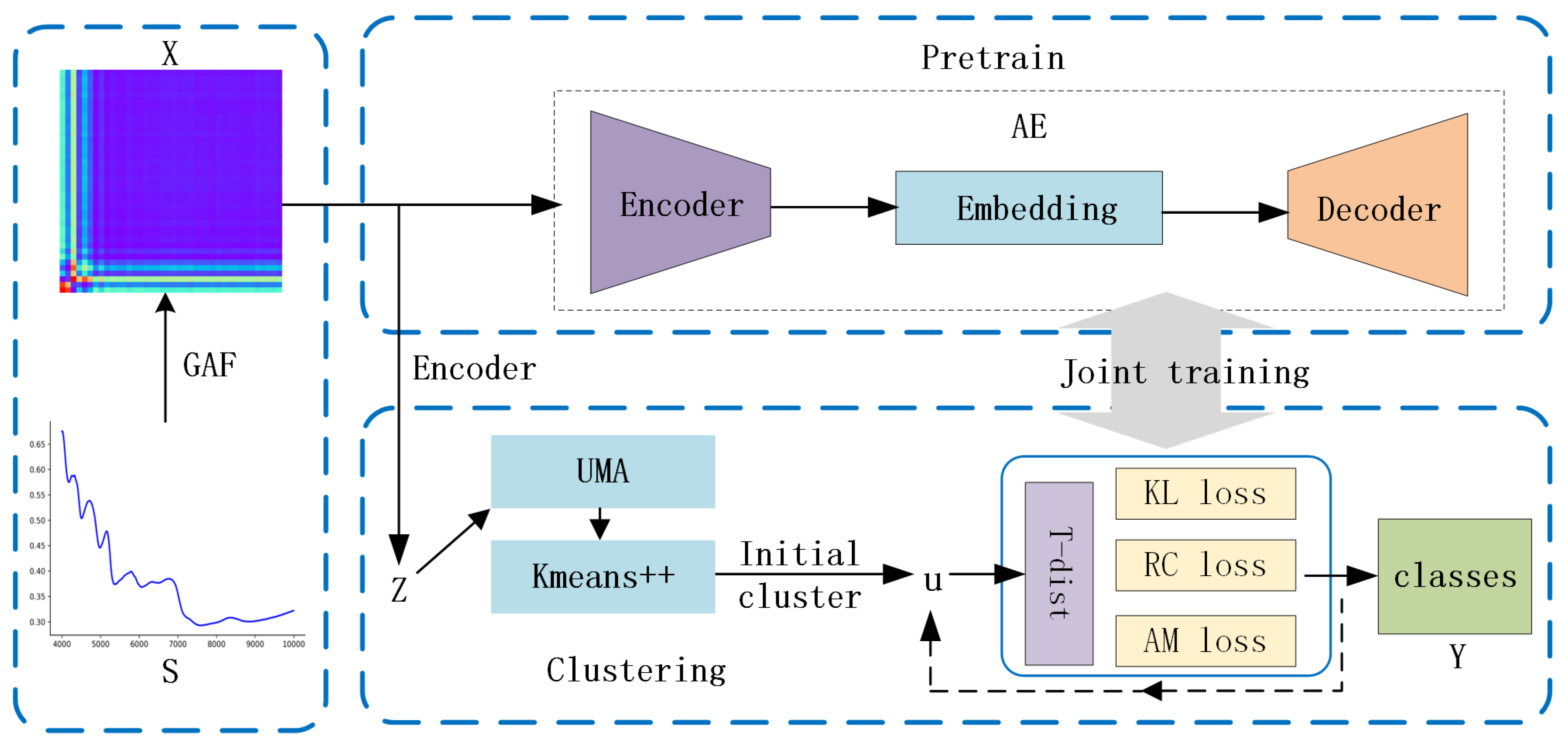
The GAF-ConvDuc model, illustrated in Figure 2, consists of the following three primary modules: feature imageization, pre-training, and joint optimization. Feature imageization can capture high-dimensional neighborhood structures. The pre-trained convolutional autoencoder can obtain low-dimensional embedding features. The final model parameters and cluster allocation can be obtained by joint optimization.
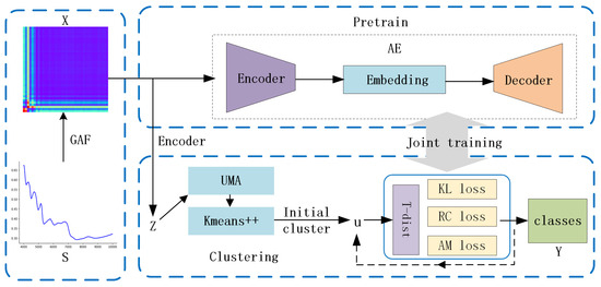
Figure 2.
The architecture of the GAF-ConvDuc clustering model.
The proposed deep clustering model involves the following specific steps:
1. Set the image size and polar coordinate mapping parameters. By using GAF, one-dimensional NIR spectra are converted into two-dimensional color images, which will serve as the input for the deep clustering algorithm.
2. During the pre-training stage, GAF images are encoded into a reduced-dimensional latent representation Z by the encoder. The reconstruction error is minimized using Adam optimization, updating the parameters of the autoencoder.
3. In the fine-tuning phase, the low-dimensional embedding representation Z serves as the input for processing the data through uniform manifold approximation. K-means++ clustering is performed on the embedding data. The initial clustering center is obtained, and then, the results are linearly mapped back to the embedding layer.
4. Calculate the soft assignment Q between data points and cluster centers, as well as the target distribution P.
5. Steps 3–4 are repeated until the loss function converges, and the cluster labels for each sample are output.
The steps of the algorithm are presented in the form of pseudo-code in Algorithm 1.
| Algorithm 1 GAF-ConvDuc |
|
4. Results and Discussion
4.1. Data and Software
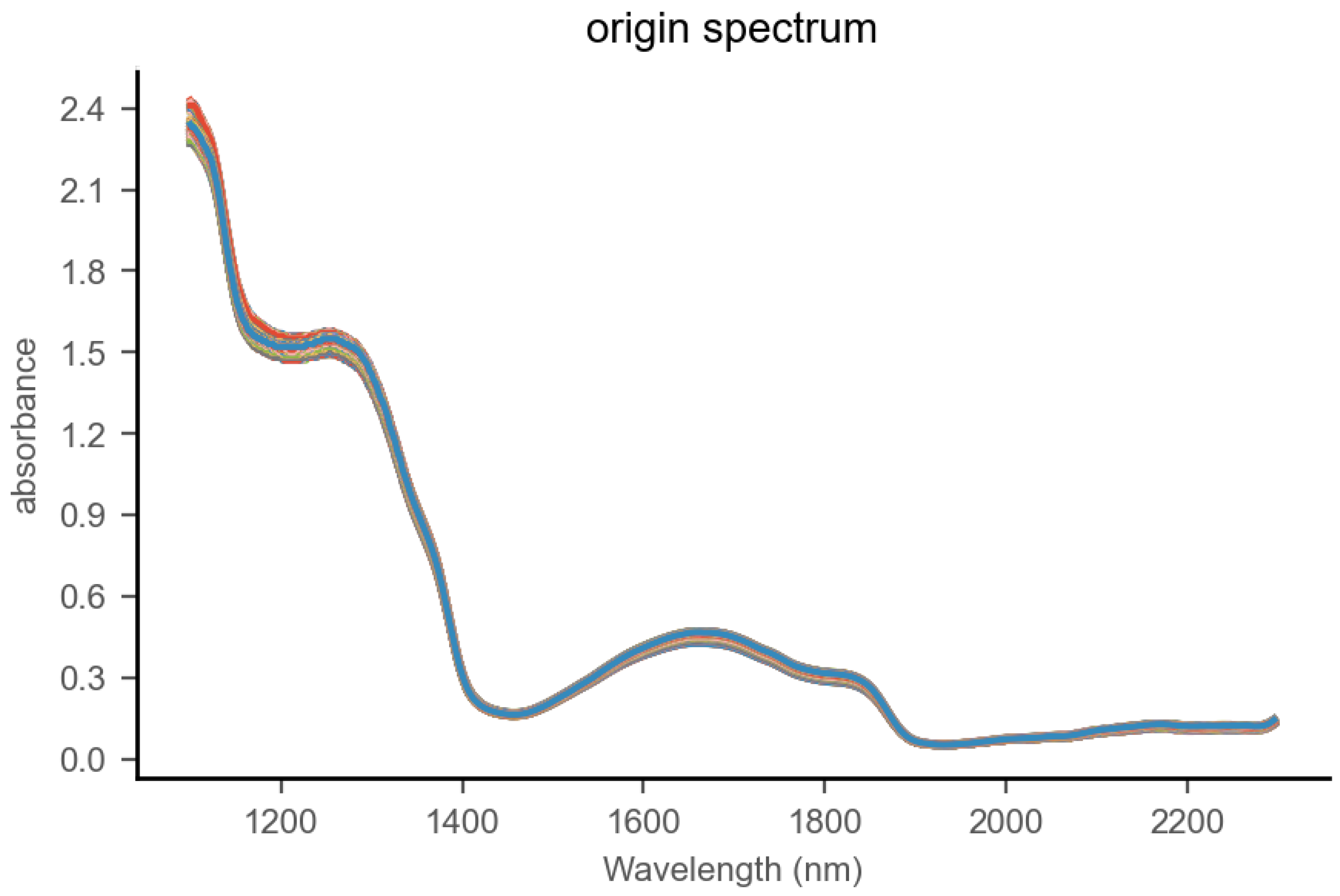
We purchased regular milk and lactose-free milk of the same brand but from different batches from the supermarket. The lactose content of the regular milk was found to be approximately 4.6%. We selected 25 samples of regular milk and 25 samples of lactose-free milk, with each sample being 200 milliliters. Using lactose-free milk as a base, we blended in regular milk at mass percentages of 0%, 12.5%, 25%, 37.5%, 50%, 62.5%, 75%, 87.5%, and 100%, where 100% means the sample contains only regular milk. The 25 samples were thoroughly mixed at different concentration gradients to produce 225 adulterated samples. Each sample was divided into 10 portions for testing, resulting in a total of 2250 adulterated samples. The samples were placed in 2-milliliter sample cups and stored at 40 ± 0.1 °C constant temperature. A 2 mm liquid optical fiber probe was adopted. The spectral range spanned from 1100 to 2300 nanometers with 2-nanometer intervals. Each sample underwent 20 scans, and the average was calculated. The spectral graph of milk samples is shown in Figure 3.
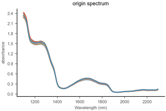
Figure 3.
Near-infrared spectrum of milk.
We collected 2250 spectral data points in the laboratory using an MPA Fourier transform near-infrared spectrometer. There are a total of nine classes, with class labels ranging from 0 to 8. A class label of 0 indicates 100% lactose-free milk, meaning 0% regular milk has been added. A class label of 1 indicates 87.5% lactose-free milk, meaning 12.5% regular milk has been added, and so on. We selected 1800 pieces of data as the training set and the remaining data as the testing set.
The experiments were performed on a system equipped with an Intel Core i7-8750H CPU (2.20 GHz) and an NVIDIA GeForce RTX 4090D GPU. Spectral preprocessing and the neural network model were implemented using Python 3.10 and PyTorch 2.1.2.
4.2. Model Performance Evaluation Metrics
The model’s performance are evaluated using clustering accuracy (ACC) [22], the Normalized Mutual Information index (NMI) [47], Adjusted Rand Index (ARI) [48], and Silhouette Coefficient (SC) [49]. The unsupervised clustering ACC is specified in Equation (11) as follows:
where is the true label, and is the predicted cluster label. is the optimization function that maps the cluster label to the true label based on the Hungarian algorithm. is the indicator function.
An ACC value close to 1 signifies excellent clustering performance, while an ACC below 0.5 indicates unsatisfactory performance. The NMI index evaluates the alignment between clustering results and true labels. An NMI value near 1 indicates high consistency with the true labels. A value near 0 suggests minimal relevance. The ARI value quantifies the similarity between true labels and clustering results, with values nearing 1 indicating greater similarity. The SC value assesses intra-cluster cohesion and inter-cluster separation. An SC value close to 1 signifies strong clustering performance, a value near 0 indicates ambiguous clustering, and a value approaching −1 denotes poor clustering performance.
4.3. Spectrum vs. Image
When acquiring NIR spectra of milk, scattering effects, baseline drift, and environmental noise can interfere with the measurement accuracy. In order to enhance the signal-to-noise ratio and spectral resolution while eliminating baseline drift and emphasizing spectral features, we adopted a processing method integrates standard normal variate (SNV), Savitzky–Golay (SG) smoothing, and first derivative preprocessing. Savitzky–Golay smoothing utilized a fifth-order polynomial with a 25-point window.
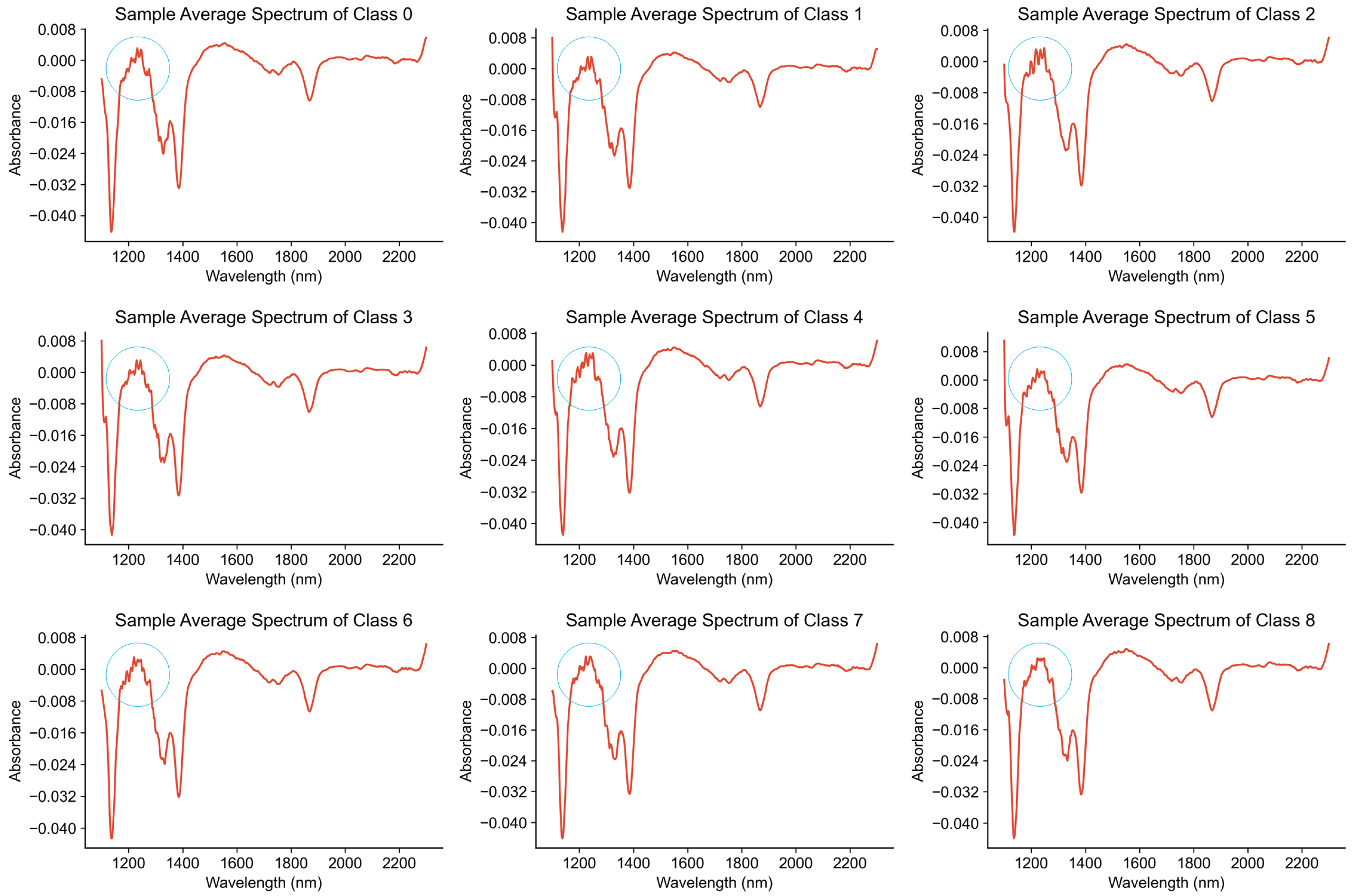
In this experiment, the adulterated milk samples are divided into nine classes, represented as class 0, class 1, through to class 8. The specific meanings are described in Section 4.1. We calculated the average of the spectra for the samples in each class to obtain the average spectrum for that class. As shown in Figure 4, in the range from 1200 to 1400 nanometers, the subtle characteristic differences in the absorption peaks of the nine types of milk spectra are highlighted. However, the absorption peaks of the spectra in other wavelength intervals are still very similar, and more effective feature extraction methods are needed to increase the discrimination of different classes.

Figure 4.
Average spectra of milk with different lactose contents.
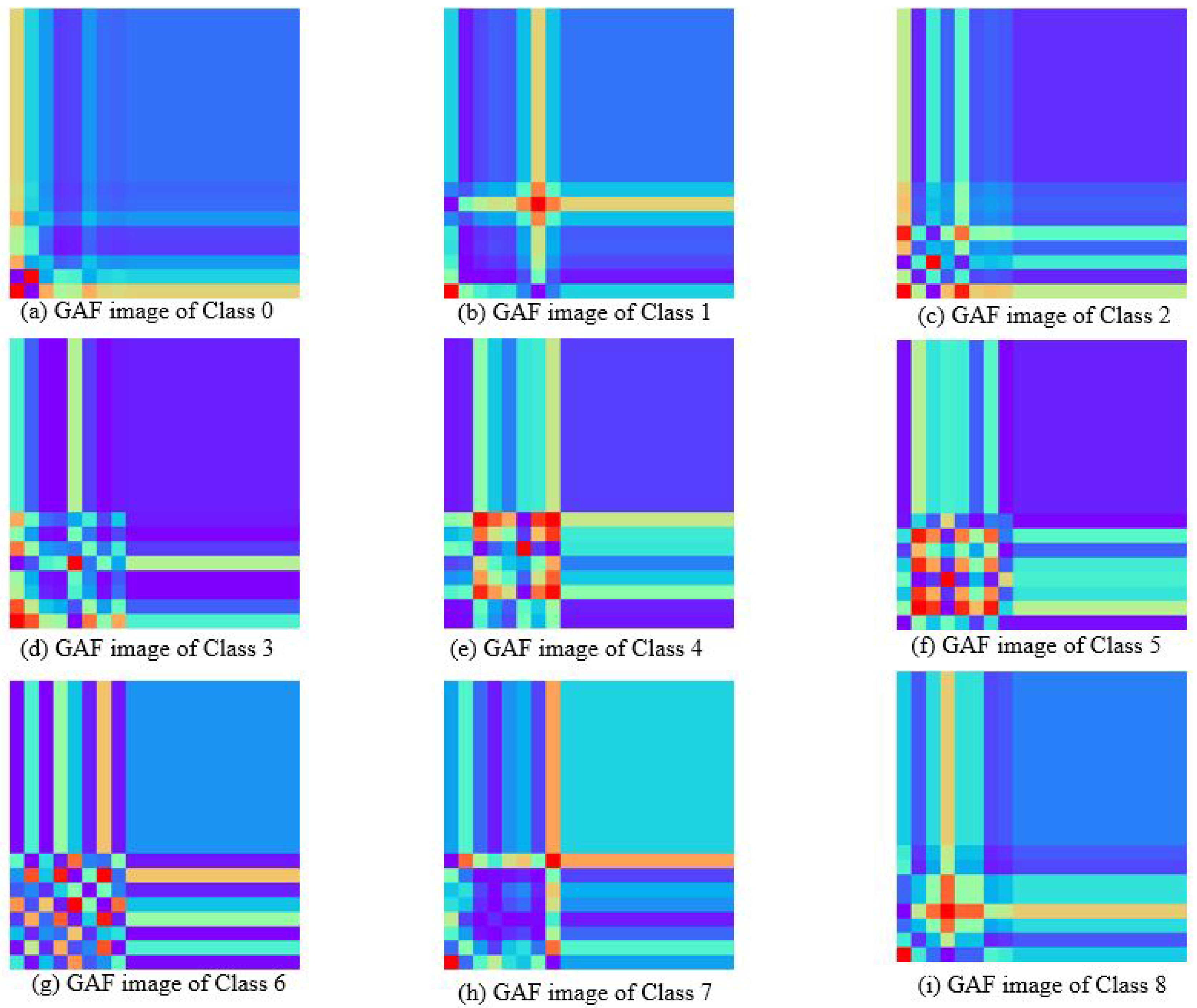
The milk spectra were transformed into two-dimensional color images using the GAF and MTF method. Figure 5 illustrates the feature images of nine types of milk samples generated through GAF. There are significant differences in the characteristics between them. GAF captures changes in time series through angle coding, it can better retain some characteristics corresponding to lactose in the original spectrum. The lower left corner of the image reflects the correlation of absorbance changes in the initial part of the spectral sequence. Classes 0, 1, and 7 exhibit small changes in this segment, while classes 4, 5, and 6 display substantial variations. The change of cross-texture indicates the difference of absorbance amplitude across different wavelength points. There are many red blocks in the GAF plots of classes 4 and 5, indicating that the corresponding lactose bands of these classes have strong correlation characteristics. There are more cross textures in classes 1, 2, 4, and 8, which correspond to the positions of the characteristic peaks in the spectrum, highlighting the important features in the original data. The absorption peaks of classes 0, 2, and 3 appear earliest, while classes 4, 6, and 7 show the latest absorption peaks.
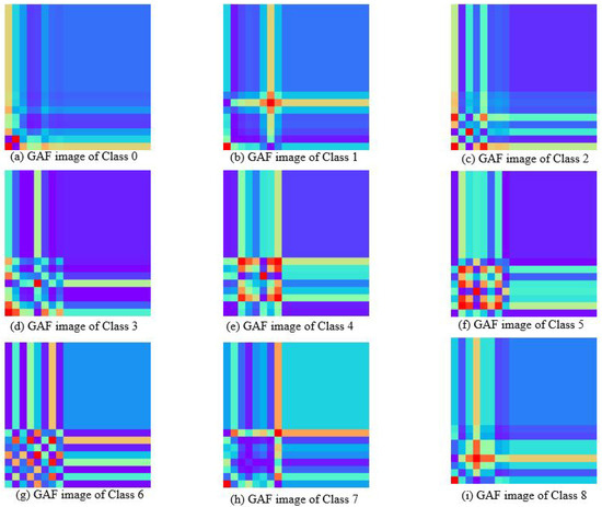
Figure 5.
Gram angular field images of milk spectra with different lactose contents.
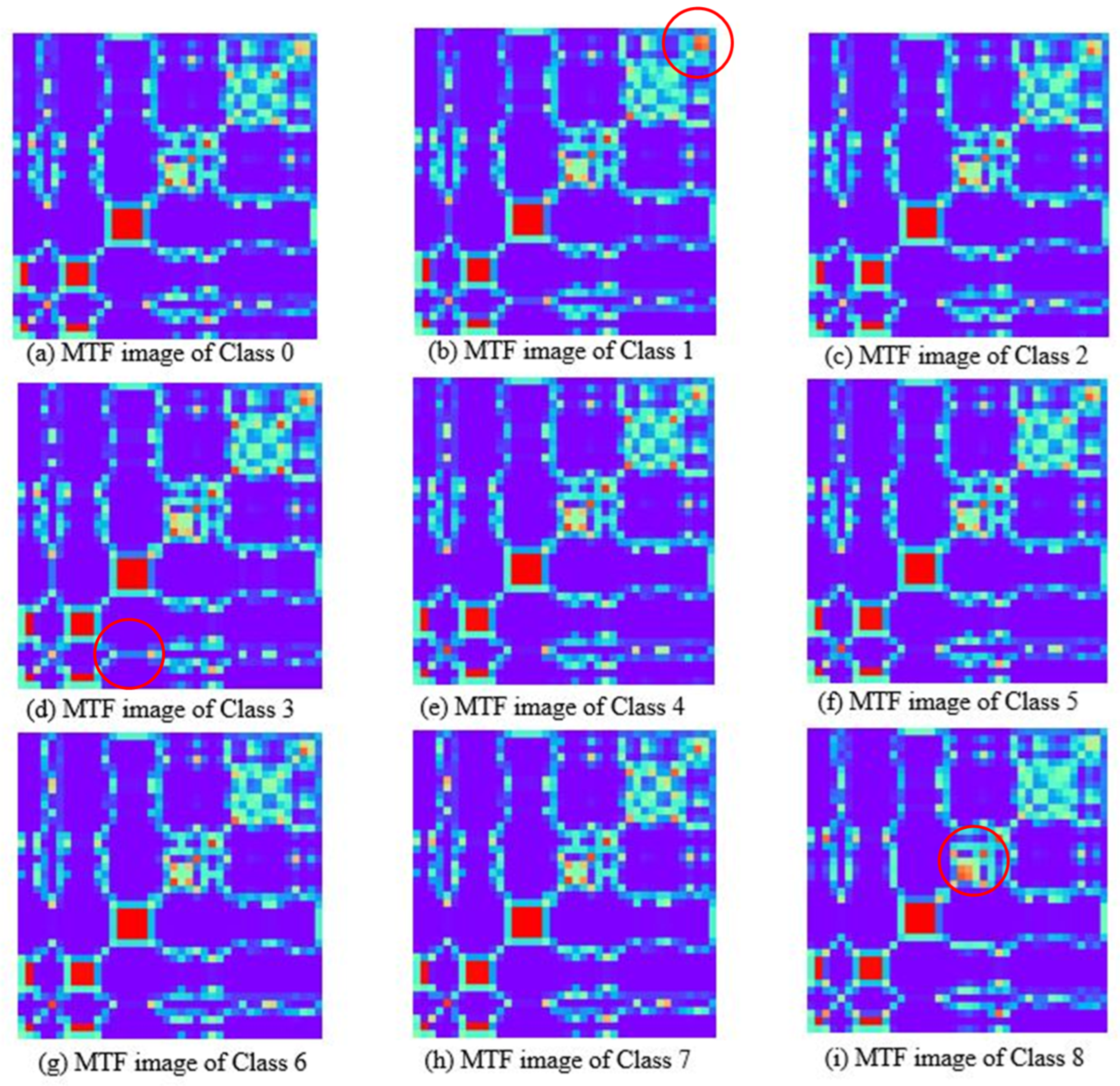
Figure 6 depicts the MTF feature images, showing that the features of most areas in the images are similar, their color and shape distributions are very close, and there are few areas with differences. Observed from the upper right corner, there are local color and texture differences among different feature images. Among them, the red circled regions in Figure 6b,d,i show that the features of classes 1, 3, and 8 exhibit high discriminability from other classes. It is indicated that the transfer probability of the average spectrum of the sample between the initial wavelength point and the intermediate wavelength point is a discriminative feature. The comparison shows that the GAF charts of the milk spectrum exhibit consistent and distinct patterns, and there are significant differences among the images of different classes. The MTF images show complex textures, and the class discrimination features contained in the images are relatively few, which poses challenges to feature extraction and recognition. The reason for this is that near-infrared spectroscopy has the characteristic of continuous variation. The state transition probabilities captured by MTF cannot better reflect the differences in the composition of substances, while GAF can more effectively reflect the minute changes of absorption peaks. Therefore, this paper selects the GAF feature image as the input of the deep clustering model, which can extract features conducive to class division through deep learning.
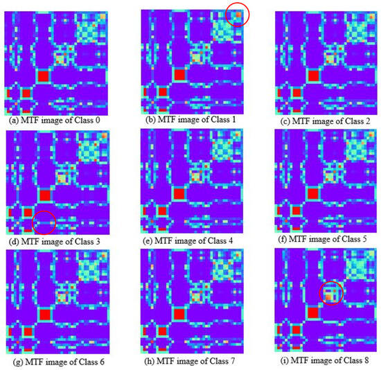
Figure 6.
Markov transition field images of milk spectra with different lactose contents.
4.4. Ablation Study of the GAF-ConvDuc Algorithm
To verify the effectiveness of the GAF and the convolutional embedding manifold clustering module, we performed an ablation study on the proposed model using a milk spectral dataset. Only one of the modules was added to each model. Each model was augmented with only one module, denoted by “w” for inclusion and “w/o” for exclusion. The baseline model employed K-means, and we compared the performance differences of these models. The experimental results are shown in Table 1.

Table 1.
Comparison of clustering performance for different module combinations.
The findings demonstrated that integrating GAF and convolutional embedding manifold clustering can significantly improve clustering performance. In comparison to the baseline K-means model, the inclusion of the GAF module led to a 9.5% increase in ACC, along with notable improvements in other metrics. This suggested that GAF transformation effectively extracted key features hidden in the time series data and improved class differentiation.
When the GAF module was not added, only the convolution embedding manifold clustering module was added, and the model’s input was the original spectral data. The model performance improved significantly. ACC rose by 14.5%, NMI increased by approximately 0.14, and SC increased by 0.38. It was indicated that K-means clustering primarily depended on original features for basic clustering. In contrast, convolutional embedding manifold clustering excelled at capturing correlations among spectral wavelengths and reducing dimensionality.
When the GAF and convolution embedding manifold clustering module were added at the same time, in comparison to the baseline model, ACC had increased by 21.7%, NMI by 0.215, ARI by 0.293, and SC by 0.462. The result indicated that convolutional embedding manifold clustering effectively captures absorption peak features and spatial structures from spectral GAF images while reducing noise interference. Following convolutional embedding, the visualization of dimensionally reduced data improved. The improved loss function and manifold clustering techniques widen the cluster separation gap and reduce clustering boundary ambiguity.
4.5. Model Performance Analysis
Key parameters within the GAF module and convolutional embedding manifold clustering module encompass feature image size, the GAF transformation method, and the embedding feature dimension. These parameters are set in different ranges, as shown in Table 2. The GAF transformation methods include two kinds as follows: GASF and GADF. The impact of modifying these parameters on the model’s performance is discussed below.
Table 2.
GAF parameters discussed.
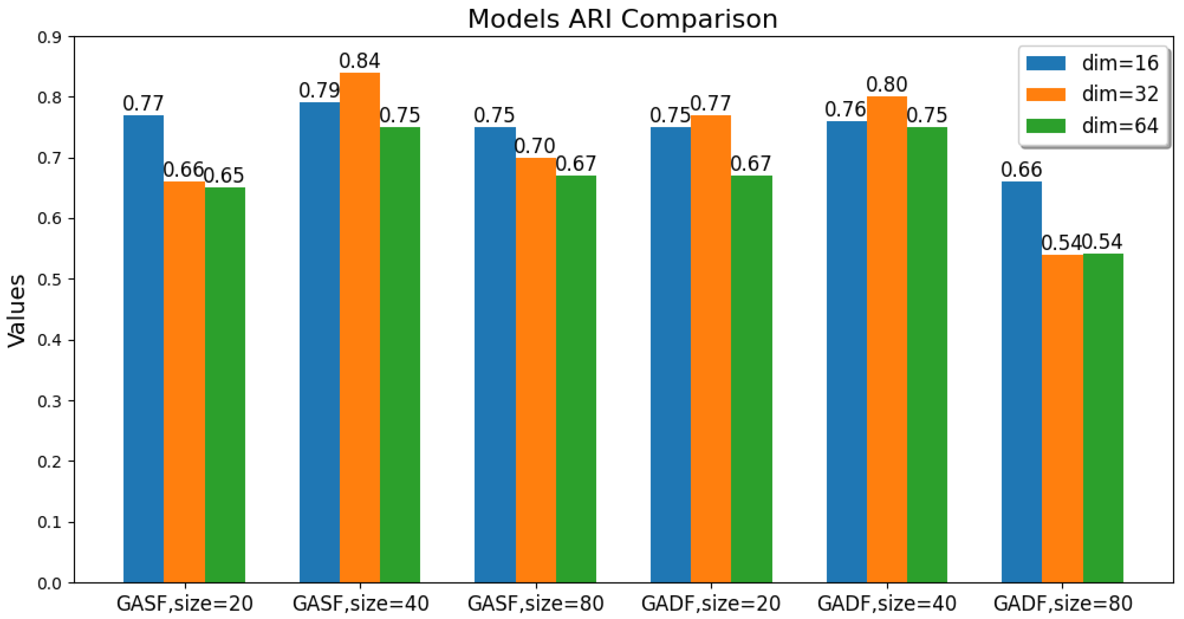
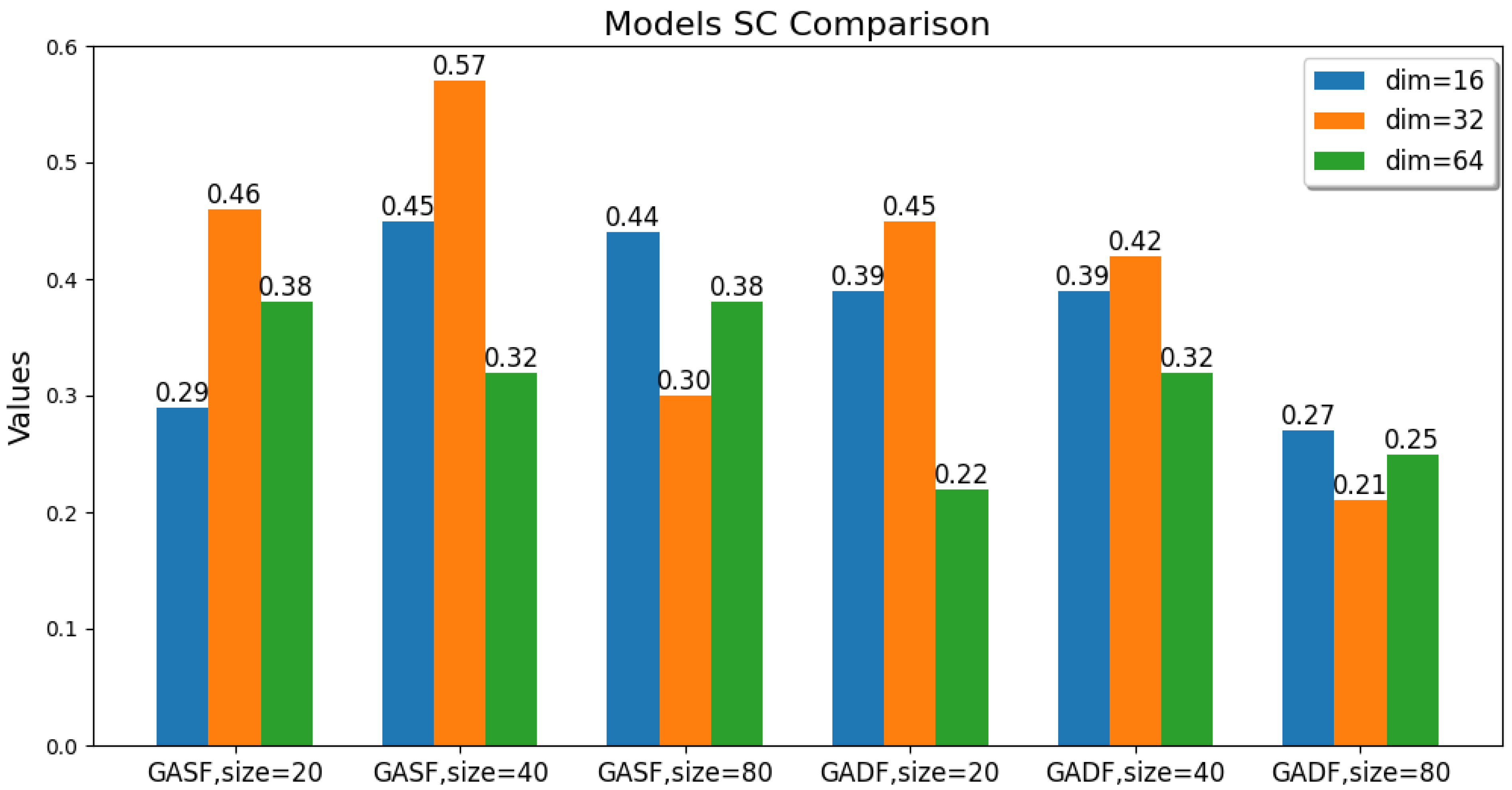
The values of these parameters, including the GAF transformation method, image size, and latent feature dimension, are changed. The ACC, ARI, and SC metric values of the GAF-ConvDuc clustering model are recorded, as shown in Figure 7, Figure 8 and Figure 9. The model performs best when the parameter combination is GASF, size = 40, and dim = 32. The clustering accuracy is 0.89, and the adjusted Rand index is 0.84, indicating a high consistency between the clustering results and the true class labels. The silhouette coefficient improves from 0.29 to 0.57, signifying a significant improvement in clustering quality, with increased intra-cluster tightness and inter-cluster separation and relatively clear boundaries.
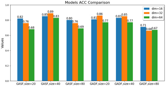
Figure 7.
Comparison of the models’ accuracy.
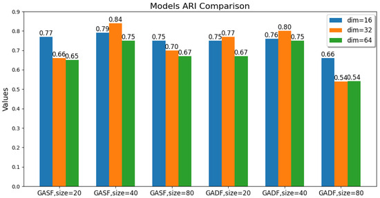
Figure 8.
Comparison of the models’ Adjusted Rand Index.
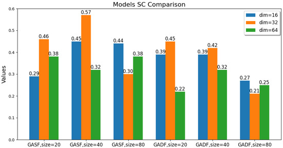
Figure 9.
Comparison of the models’ Silhouette Coefficient.
Overall, the clustering models based on GASF-generated images generally outperform those based on GADF. This is because GASF-generated images can better preserve the amplitude information of the original spectral points, retaining the height, width, and position of absorption peaks more effectively and highlighting the peaks with stronger intensities. Although GADF-generated images can emphasize high-frequency information and local changes in the spectrum, some key features are lost during the subtraction process, making deep clustering models more sensitive to noise and minor variations, thus leading to a decline in clustering performance.
A special case is when the generated image size is 20 and the performance of the clustering model obtained from GASF is inferior to that from GADF. The reason is that GAF image size is too small, the GASF method results in a significant loss of intensity information from the original spectrum, but GADF captures the relative changes and shape differences of the spectrum, and its image patterns can more clearly reflect the differences between classes. When the GAF image size is too small, the information about the shape and peak position shifts in the absorption peaks in the original spectrum is significantly compressed, causing the convolutional autoencoder to be unable to effectively learn multi-scale features. Additionally, when the image size is too large, the computational burden increases significantly, and there is an increase in redundant information and noise. The convolutional autoencoder is forced to learn and encode this information, leading to a decline in model accuracy. The clustering silhouette coefficient significantly decreases, mainly because the feature space dimension extracted by the convolutional autoencoder is too high, failing to form tight and well-separated clusters.
During the training of the GAF-ConvDuc model, the network parameters and clustering centers are iteratively optimized, with the goal of minimizing the loss function and the intra-cluster distance. To prevent the model from overfitting or underfitting, it was trained for 600 epochs, and the training and validation set loss were recorded, as shown in Figure 10. Model training adopts a learning rate of = 0.001, embedding a feature dimension of dim = 32, utilizing the Adam optimizer.
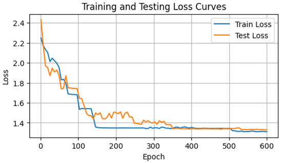
Figure 10.
Loss curve of GAF-ConvDuc.
Based on the loss curves of the training and validation sets, the loss value drops rapidly within the first 100 iterations. Between 200 and 300 iterations, the validation loss experiences a slight increase. With Adam optimization, the loss value resumes declining, suggesting improved clustering performance and more suitable assignment of data points to clusters. After 400 iterations, the algorithm starts to converge, displaying no indications of overfitting.
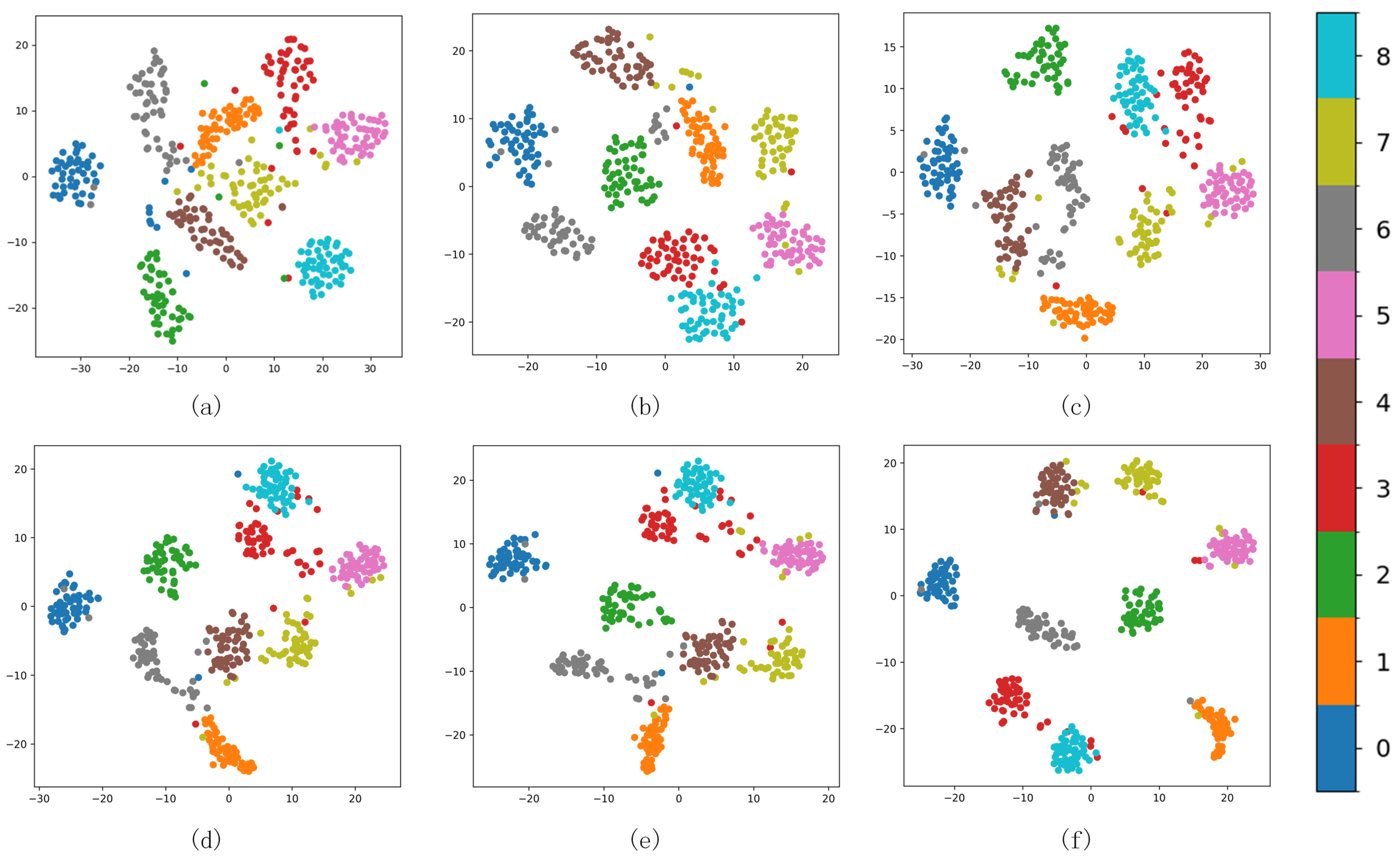
As shown in Figure 11 from (a) to (f), it can be seen that, initially, the boundaries between the nine clusters are seriously confused. As the number of iterative optimization steps increases, the distances between different types of milk samples are also increasing. With continuous optimization, ambiguous boundary points in Figure 11c progressively migrate towards the true class centers, intra-cluster data distributions become markedly denser. In Figure 11f, only a few samples are confused. It demonstrates that integrating uniform manifold approximation with K-means++ clustering enhances the initial clustering centers. During the joint clustering optimization, the incorporation of an adaptive margin loss sharpens the boundaries between classes, thereby improving both inter-cluster separation and intra-cluster cohesion.
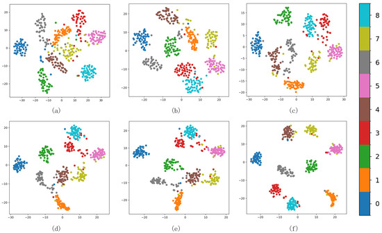
Figure 11.
Cluster changes of different epochs in the iterative process (a) 0, (b) 100, (c) 200, (d) 350, (e) 500, and (f) 600.
We compare model performance using eight benchmark models and GAF-ConvDuc. These eight models are obtained by combining feature visualization methods with traditional clustering and deep clustering methods, respectively. GAF and MTF are selected for feature visualization. The model training uses the optimal parameters and the five-fold cross-validation method, with the results presented in Table 3.
Table 3.
Clustering performance evaluation: traditional vs. deep learning algorithms for detection of lactose content in milk.
The analysis reveals that the traditional clustering algorithm is generally inferior to the deep clustering algorithm on the milk spectral dataset. The clustering quality of spectra after GAF transformation is better than the original spectral clustering results, and it is also better than the clustering after MTF transformation. The GAF-Kmeans clustering algorithm is the best performance model among traditional clustering. In the deep clustering algorithm, VAE uses the autoencoder of the feedforward network to extract features directly from the original spectrum. Its performance is slightly lower than that of GAF-DEC model, and its accuracy reaches 81.7%. The latter uses a convolutional autoencoder, which is superior to the former in its ability to extract local features of spectral images.
Our proposed GAF-ConvDuc model has the best overall performance, with the ACC value reaching 88.9% and the SC value increasing to 0.571. Compared with VAE deep clustering, ACC and SC increased by 7.2% and 0.101, respectively. The data suggest that the clustering results of milk spectra are highly consistent with the real labels, and most of the samples can be assigned to the correct classes. The SC value is lower, which indicates that the inter-cluster separation and intra-cluster cohesion is small, and there are some overlapping clusters.
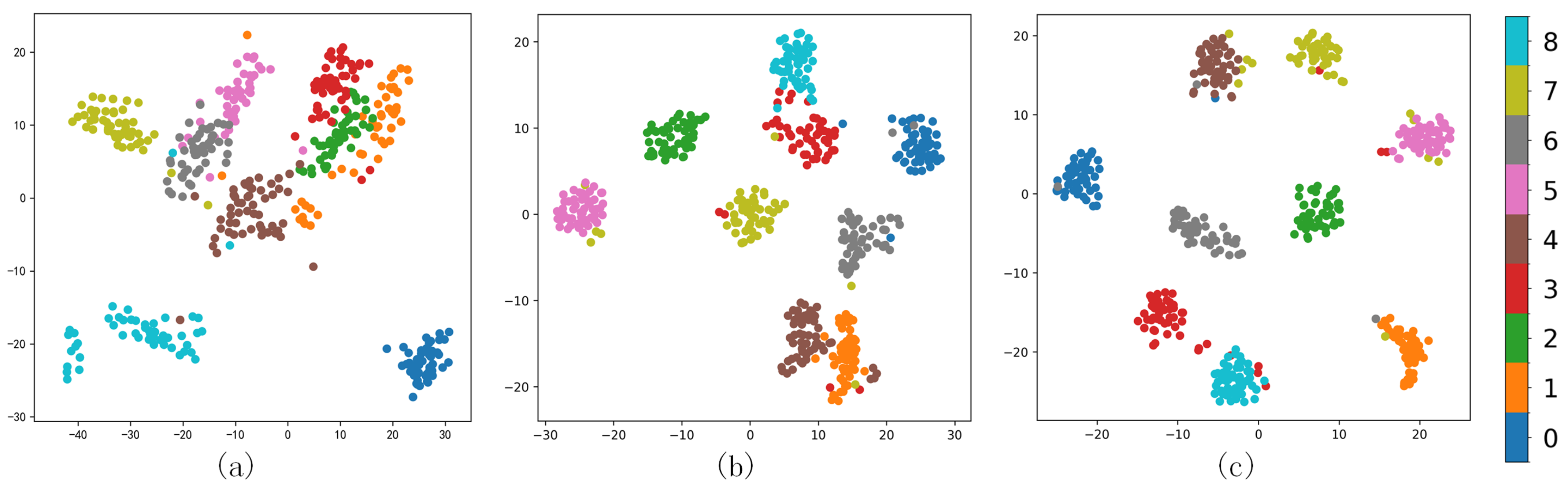
We further analyzed the clustering effect of the GAF-Kmeans, VAE, and GAF-ConvDuc models on nine types of milk samples. The milk spectral data were clustered and projected onto a two-dimensional plane to observe whether different clusters were clearly separated and evaluate the quality differences of different clusters, as shown in Figure 12.
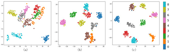
Figure 12.
Different methods’ comparison (a) GAF-Kmeans, (b) VAE, and (c) GAF-ConvDuc.
For milk spectral data with complex cluster shapes, the projection graph of GAF-Kmeans clustering results shows that there are many overlapping data points in the clustering boundary of traditional clustering methods. Especially for the samples of class 1, 2, and 3, the inter-cluster separation is low, so the silhouette coefficient is low. The VAE clustering results show that the inter-cluster separation has increased, and the boundary ambiguity problem is improved to a certain extent, but the intra-cluster cohesion is only slightly increased, and some samples of classes 2 and 3 are still confused in other classes. GAF-ConvDuc clustering not only increases the inter-cluster separation, but it also increases the intra-cluster cohesion and separates samples of different classes more clearly.
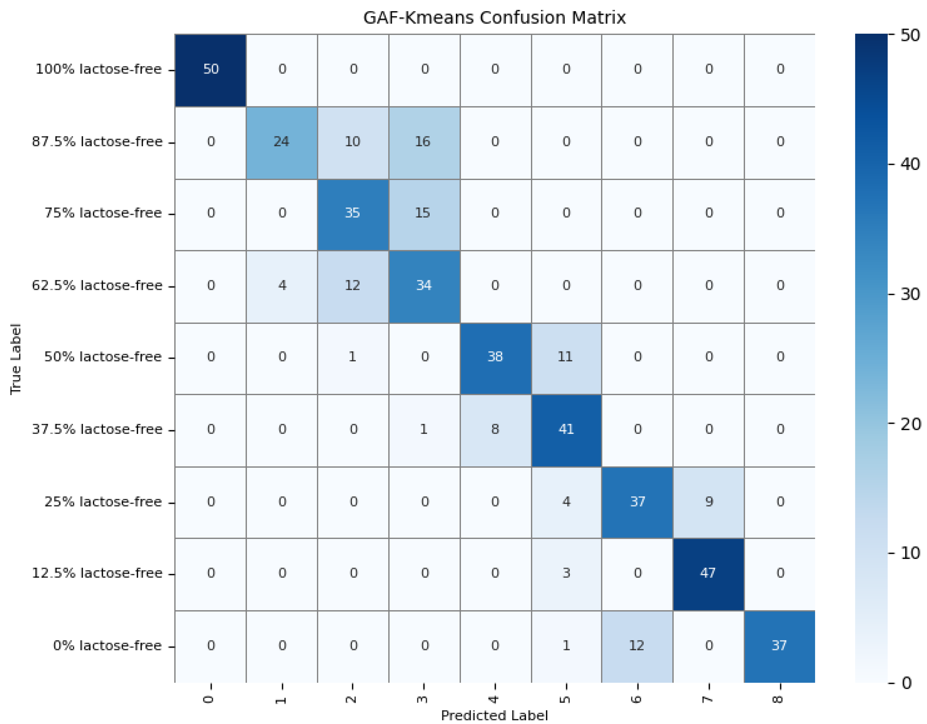
To further understand the model’s detection accuracy on different types of milk samples, 450 randomly selected test samples were predicted using the GAF-Kmeans, VAE, and GAF-ConvDuc models, respectively. The confusion matrices are shown in Figure 13, Figure 14 and Figure 15.
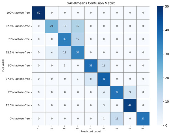
Figure 13.
Confusion matrix of the GAF-Kmeans model.
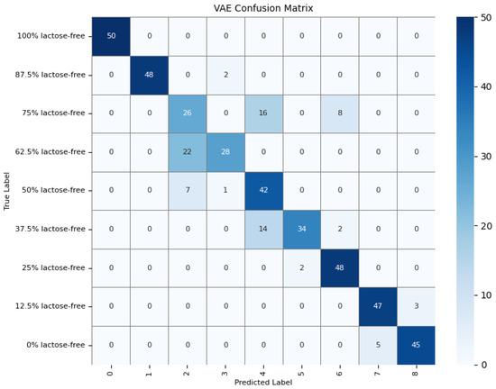
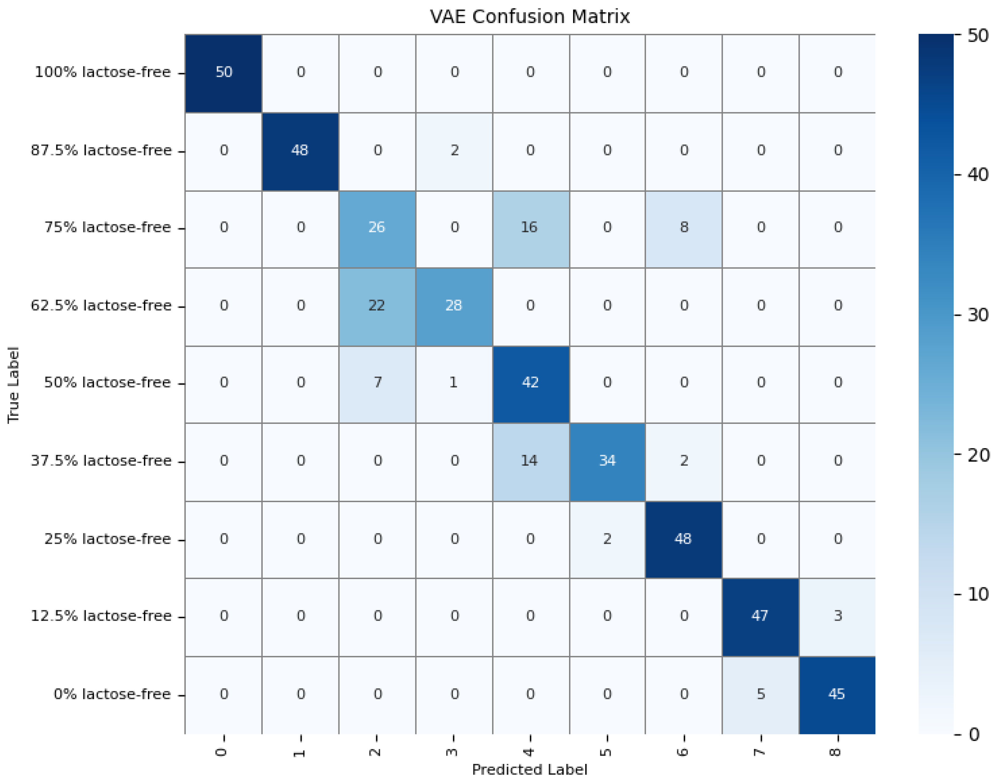
Figure 14.
Confusion matrix of the VAE model.

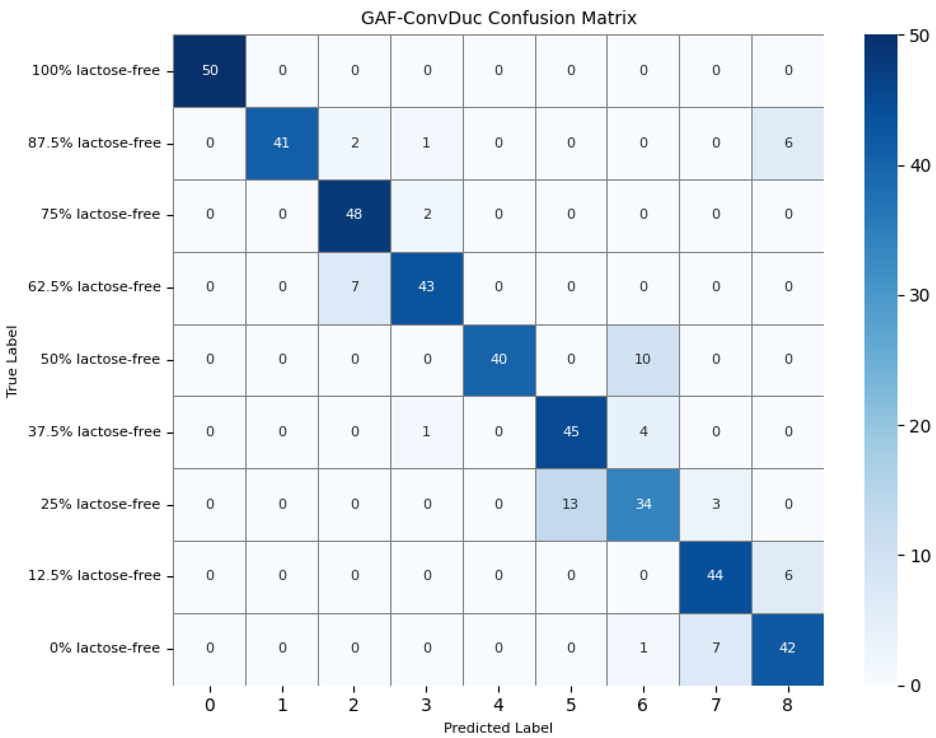
Figure 15.
Confusion matrix of the GAF-ConvDuc model.
The results indicate that 100% lactose-free milk samples can be correctly identified by all three models. The total number of misclassified samples for the GAF-Kmeans, VAE, and GAF-ConvDuc models are 95, 71, and 63, respectively. GAF-ConvDuc model performs the best. GAF-Kmeans model has an average precision of 0.786, a recall of 0.762, and an F1-score of 0.764. The VAE model has an average precision of 0.841, a recall of 0.818, and an F1-score of 0.819. The GAF-ConvDuc model has an average precision of 0.879, a recall of 0.86, and an F1-score of 0.871. The proposed model achieves the highest recall, reducing the rate of missed detections of adulterated samples.
The GAF-Kmeans model has a higher error rate when identifying adulterated samples containing 87.5%, 75%, and 62.5% lactose-free milk. The VAE model has a higher error rate when identifying adulterated samples containing 75% and 62.5% lactose-free milk. The GAF-ConvDuc model has a higher error rate when identifying adulterated samples containing 25% lactose-free milk. Compared to the GAF-Kmeans model, the model proposed in this paper shows the greatest improvement in detection accuracy for samples containing 87.5%, 75%, and 62.5% lactose-free milk, with increases of 34%, 26%, and 18%, respectively. This indicates that after GAF transformation and deep manifold clustering, the model is able to extract subtle compositional differences and correctly distinguish the features of different classes of samples.
4.6. Model Complexity Analysis
In order to evaluate the computational requirements and efficiency of the clustering algorithm, the accuracy, computational complexity, and running time of the five models are compared in Table 4.
Table 4.
Complexity of different models.
The results show that compared with the deep clustering method, the traditional clustering model has significant advantages in training time and prediction time. K-means clustering directly on raw milk spectra takes only 1.28 s and prediction takes only 0.13 s. This model has the lowest complexity and also the lowest accuracy. K-means clustering’s time complexity is associated with the sample count, class number, input dimension, and iteration count. The time complexity of the deep clustering model is related to the network structure, potential spatial dimension, and number of classes, so the computational complexity is higher than that of traditional methods. In terms of clustering accuracy, the deep clustering model is superior to traditional clustering. It is more suitable for processing high-dimensional NIR data.
The accuracy of the VAE clustering model is not the best, but its computational efficiency is better than that of the GAF-ConvDuc model. VAE has a simpler structure and does not require the optimization of cluster centers. If the computing resources and clustering accuracy are considered comprehensively, VAE is a better choice. The GAF-ConvDuc model has the highest complexity, with MFLOPs of 19.18 and training time of 43.82 s. However, it performs best in accuracy. In general, this computing resource requirement is relatively easy to meet, so considering that the goal of lactose-free milk adulteration detection is high-precision identification, the GAF-ConvDuc model is a better choice. Although the training time of the GAF-ConvDuc model is longer than that of the traditional clustering model, its testing time is within a few seconds and it can be applied in engineering. The model generated based on the PyTorch framework is relatively small, only 12.7 MB, and can be deployed to hardware devices through the NVIDIA Jetson platform.
5. Conclusions
In this study, we introduce a method for detecting lactose-free milk adulteration based on deep clustering. Our method demonstrates enhanced accuracy and robustness, achieving an accuracy rate of 88.9%. By transforming the intricate spectral data dynamics into image spatial structures, the convolutional autoencoder effectively captures low-dimensional embedding features that retain crucial information, including the location and strength of absorption peaks in the spectrum. Furthermore, the improvements in initial clustering and loss function make the clustering boundaries clearer.
Future work will focus on feature selection, model generalizability across different devices, and real-time model deployment. Advanced heuristic feature subset selection methods will be studied to extract key features that have a significant impact on classification tasks. Near-infrared spectroscopy data from different devices are collected, and model transfer methods are combined to improve the prediction accuracy of the model across various devices. We plan to explore model quantization and hardware acceleration methods with the aim of deploying the model on a portable near-infrared spectrometer to further enhance the efficiency of milk adulteration detection.
In summary, the outcomes of this study have improved the accuracy of milk adulteration detection in the absence of labeled data, providing an effective solution for food safety supervision.
Author Contributions
Conceptualization, C.Z. and Y.H.; methodology, C.Z. and S.D.; software, C.Z. and S.D.; validation, C.Z.; formal analysis, C.Z.; investigation, S.D.; writing—original draft preparation, C.Z.; writing—review and editing, Y.H. and S.D. All authors have read and agreed to the published version of the manuscript.
Funding
This research received no external funding.
Institutional Review Board Statement
This is not applicable for studies not involving humans or animals.
Informed Consent Statement
Not applicable.
Data Availability Statement
The data presented in this study are available from the first author upon request.
Conflicts of Interest
The authors declare no conflicts of interest.
References
- Ren, Q.; Zhang, H.; Guo, H.; Jiang, L.; Tian, M.; Ren, F. Detection of cow milk adulteration in yak milk by ELISA. J. Dairy Sci. 2014, 97, 6000–6006. [Google Scholar] [CrossRef] [PubMed]
- Poonia, A.; Jha, A.; Sharma, R.; Singh, H.B.; Rai, A.K.; Sharma, N. Detection of adulteration in milk: A review. Int. J. Dairy Technol. 2017, 70, 23–42. [Google Scholar] [CrossRef]
- Tsakali, E.; Agkastra, C.; Koliaki, C.; Livanios, D.; Boutris, G.; Christopoulou, M.I.; Koulouris, S.; Koussissis, S.; Impe, J.F.M.V.; Houhoula, D. Milk Adulteration: Detection of Bovine Milk in Caprine Dairy Products by Real Time PCR. J. Food Res. 2019, 8, 52. [Google Scholar] [CrossRef]
- Harini, V.; Meher, S.; Alex, Z. A novel refractive index based-fiber optic sensor for milk adulteration detection. Opt. Mater. 2024, 154, 115810. [Google Scholar] [CrossRef]
- Feng, Y.; Zhang, Y. Rapid ATR-FTIR Principal Component Analysis of Commercial Milk. Spectrosc. Spectr. Anal. 2023, 43, 838–841. [Google Scholar]
- Huang, Y.; Guo, X.; Tang, G.; Xiong, Y.; Min, S. Quantitative Analysis of Urea Adulteration in Milk by Near-Infrared Spectroscopy. Spectrosc. Spectr. Anal. 2023, 43, 65–66. [Google Scholar]
- Wei, Y.; Li, L.; Yang, X.; Li, D.; Fu, H.; Yang, T. Near-Infrared Spectroscopy Pattern Recognition of Melamine-Adulterated Milk. China Dairy Ind. 2016, 44, 48–51. [Google Scholar]
- Farah, J.S.; Cavalcanti, R.N.; Guimarães, J.T.; Balthazar, C.F.; Coimbra, P.T.; Pimentel, T.C.; Esmerino, E.A.; Duarte, M.C.K.; Freitas, M.Q.; Granato, D.; et al. Differential scanning calorimetry coupled with machine learning technique: An effective approach to determine the milk authenticity. Food Control 2021, 121, 107585–107593. [Google Scholar] [CrossRef]
- Cai, L.; Zheng, Y.; Liu, Y.; Zhou, R.; Ma, M. Near-infrared (NIR) spectroscopy combined with chemometrics for qualitative and quantitative detection of camel milk powder adulteration. J. Food Compos. Anal. 2025, 143, 107571. [Google Scholar] [CrossRef]
- Wu, X.; Fang, Y.; Wu, B.; Liu, M. Application of Near-Infrared Spectroscopy and Fuzzy Improved Null Linear Discriminant Analysis for Rapid Discrimination of Milk Brands. Foods 2023, 12, 3929. [Google Scholar] [CrossRef]
- Yu, G.; Ma, B.; Chen, J.; Dang, F.; Li, X.; Li, C.; Wang, G. Discrimination Method of Pesticide Residues on Hami Melon Surface Based on GADF Transform and Multi-scale CNN Using Visible-Near Infrared Spectroscopy. Spectrosc. Spectr. Anal. 2021, 41, 3701–3707. [Google Scholar]
- Neto, H.A.; Tavares, W.L.; Ribeiro, D.C.; Alves, R.C.; Fonseca, L.M.; Campos, S.V. On the utilization of deep and ensemble learning to detect milk adulteration. BioData Min. 2019, 12, 1–13. [Google Scholar] [CrossRef] [PubMed]
- Chu, C.; Wang, H.; Luo, X.; Fan, Y.; Nan, L.; Du, C.; Gao, D.; Wen, P.; Wang, D.; Yang, Z.; et al. Rapid detection and quantification of melamine, urea, sucrose, water, and milk powder adulteration in pasteurized milk using Fourier transform infrared (FTIR) spectroscopy coupled with modern statistical machine learning algorithms. Heliyon 2024, 10, e32720. [Google Scholar] [CrossRef] [PubMed]
- Rashvand, M.; Paterna, G.; Laveglia, S.; Zhang, H.; Shenfield, A.; Gioia, T.; Altieri, G.; Renzo, G.C.D.; Genovese, F. Quality detection of common beans flour using hyperspectral imaging technology: Potential of machine learning and deep learning. J. Food Compos. Anal. 2025, 142, 107424. [Google Scholar] [CrossRef]
- Ninh, D.K.; Phan, K.D.; Vo, C.T.; Dang, M.N.; Thanh, N.L. Classification of Histamine Content in Fish Using Near-Infrared Spectroscopy and Machine Learning Techniques. Information 2024, 15, 528. [Google Scholar] [CrossRef]
- Zain, S.M.; Behkami, S.; Bakirdere, S.; Koki, I.B. Milk authentication and discrimination via metal content clustering—A case of comparing milk from Malaysia and selected countries of the world. Food Control 2016, 66, 306–314. [Google Scholar] [CrossRef]
- Crase, S.; Hall, B.; Thennadil, S.N. Cluster Analysis for IR and NIR Spectroscopy: Current Practices to Future Perspectives. Comput. Mater. Contin. 2021, 69, 1945–1965. [Google Scholar] [CrossRef]
- Buoio, E.; Colombo, V.; Ighina, E.; Tangorra, F. Rapid Classification of Milk Using a Cost-Effective Near Infrared Spectroscopy Device and Variable Cluster-Support Vector Machine (VC-SVM) Hybrid Models. Foods 2024, 13, 3279. [Google Scholar] [CrossRef]
- Guan, C.; Liang, S.; Chen, J.; Wang, Z. Research on Split-Type LIBS Detection Method for Soil Heavy Metals Based on Clustering Analysis. Spectrosc. Spectr. Anal. 2024, 44, 2506–2513. [Google Scholar]
- Rumelhart, D.E.; Hinton, G.E.; Williams, R.J. Learning representations by back-propagating errors. Nature 1986, 323, 533–536. [Google Scholar] [CrossRef]
- Kingma, D.P.; Welling, M. Auto-encoding variational bayes. arXiv 2013, arXiv:1312.6114. [Google Scholar] [CrossRef]
- Xie, J.; Girshick, R.B.; Farhadi, A. Unsupervised Deep Embedding for Clustering Analysis. arXiv 2015, arXiv:1511.06335. [Google Scholar] [CrossRef]
- Jo, S.; Sohng, W.; Lee, H.; Chung, H. Evaluation of an autoencoder as a feature extraction tool for near-infrared spectroscopic discriminant analysis. Food Chem. 2020, 331, 127332. [Google Scholar] [CrossRef] [PubMed]
- Hu, D.; Niu, H.; Wang, G.; Karimi, H.R.; Liu, X.; Zhai, Y. Planetary gearbox fault classification based on tooth root strain and GAF pseudo images. ISA Trans. 2024, 153, 11–15. [Google Scholar] [CrossRef]
- Lei, C.; Wang, L.; Zhang, Q.; Li, X.; Feng, R.; Li, J. Rolling bearing fault diagnosis method based on MTF and PC-MDCNN. J. Mech. Sci. Technol. 2024, 38, 3315–3325. [Google Scholar] [CrossRef]
- Zhao, C.; Yin, Z.; Zhang, W.; Guo, P.; Ma, Y. Identification of apple watercore based on ConvNeXt and Vis/NIR spectra. Infrared Phys. Technol. 2024, 142, 105575. [Google Scholar] [CrossRef]
- Liu, Q.; Zhang, J.; Lin, S.; Yu, P.; Liu, Z.; Guan, X.; Huang, J. Discriminating moisture content in Fraxinus mandshurica Rupr logs using fusion of 2D GADF spectral images and 1D NIR spectra. Microchem. J. 2025, 208, 112394. [Google Scholar] [CrossRef]
- Deng, J.; Chen, Z.; Jiang, H.; Chen, Q. High-precision detection of dibutyl hydroxytoluene in edible oil via convolutional autoencoder compressed Fourier-transform near-infrared spectroscopy. Food Control 2025, 167, 110808. [Google Scholar] [CrossRef]
- Yuan, Z.; Dong, D. Near-Infrared Spectroscopy Measurement with Contrasted Variational Autoencoders and Its Application in Liquid Sample Detection. Spectrosc. Spectr. Anal. 2022, 42, 3637–3641. [Google Scholar]
- Du, S.; Han, W.; Kang, Z.; Liao, Y.; Li, Z. A Convolution Auto-Encoders Network for Aero-Engine Hot Jet FT-IR Spectrum Feature Extraction and Classification. Aerospace 2024, 11, 933. [Google Scholar] [CrossRef]
- Bai, Y.; Sun, X.; Ji, Y.; Fu, W.; Zhang, J. Two-stage multi-dimensional convolutional stacked autoencoder network model for hyperspectral images classification. Multimed. Tools Appl. 2023, 83, 23489–23508. [Google Scholar] [CrossRef]
- Li, M.; Cao, C.; Li, C.; Yang, S. Deep Embedding Clustering Based on Residual Autoencoder. Neural Process. Lett. 2024, 56, 127. [Google Scholar] [CrossRef]
- Bai, Y.; Zhou, Y.; Liu, J. Clustering Analysis of Daily Load Curves Based on Deep Convolutional Embedded Clustering. Power Syst. Technol. 2022, 46, 2104–2113. [Google Scholar] [CrossRef]
- Duan, L.; Ma, S.; Aggarwal, C. Improving spectral clustering with deep embedding, cluster estimation and metric learning. Knowl. Inf. Syst. 2021, 63, 675–694. [Google Scholar] [CrossRef]
- Feng, L.; Wang, C.; Wu, T.; Zhang, J. Dimensionality Reduction Method Based on Manifold Learning with Variational Autoencoder. J. Comput.-Aided Des. Comput. Graph. 2025, 37, 439–445. [Google Scholar]
- Nie, P.; Xiao, H.; Yu, C. Improved Model of YOLOv5 Prediction Bounding Box Clustering Adaptive Loss Weight. Control Decis. 2023, 38, 645–653. [Google Scholar] [CrossRef]
- Li, Q.; Zou, Y.; Long, G.H.; Wu, W. Ferromagnetic resonance over-voltage identification method based on Gram angle field. Energy Rep. 2022, 8, 546–558. [Google Scholar] [CrossRef]
- Hu, Y.; Luo, P.; Liu, H.; Shi, P.; Jiang, N.; Deng, Q.; Liu, S.; Zhou, J.; Han, H. Open-circuit fault diagnosis method of inverter in wind turbine yaw system based on GADF image coding. Comput. Electr. Eng. 2024, 117, 109252–109263. [Google Scholar] [CrossRef]
- Cheng, X.; Zhang, Z.; Bao, Y.; Zheng, H. Identification of High-Risk Scenarios for Cascading Failures in New Energy Power Grids Based on Deep Embedding Clustering Algorithms. Energy Eng. 2023, 120, 2517–2529. [Google Scholar] [CrossRef]
- Becht, E.; Mcinnes, L.; Healy, J.; Dutertre, C.A.; Kwok, I.W.H.; Ng, L.G.; Ginhoux, F.; Newell, E.W. Dimensionality reduction for visualizing single-cell data using UMAP. Nat. Biotechnol. 2018, 37, 38–43. [Google Scholar] [CrossRef]
- Ireneusz, S.; Anna, S.C.; Marek, F.; Paulina, J. Dimensionality reduction by UMAP for visualizing and aiding in classification of imaging flow cytometry data. iScience 2022, 25, 105142. [Google Scholar] [CrossRef]
- Zhao, H.; Yang, Y. The research on two phase pickup vehicle routing based on the K-means++ and genetic algorithms. Int. J. Web Eng. Technol. 2020, 15, 32–52. [Google Scholar] [CrossRef]
- Wu, Z.; Fang, G.; Wang, Y.; Xu, R. An End-to-end Deep Clustering Method with Consistency and Complementarity Attention Mechanism for Multisensor Fault Diagnosis. Appl. Soft Comput. 2024, 158, 111594. [Google Scholar] [CrossRef]
- Ji, S.; Zhu, H.; Wang, P.; Ling, X. Image clustering algorithm using superpixel segmentation and non-symmetric Gaussian–Cauchy mixture model. IET Image Process. 2020, 14, 4132–4143. [Google Scholar] [CrossRef]
- Kouser, K.; Priyam, A.; Gupta, M.; Kumar, S.; Bhattacharjee, V. Genetic Algorithm-Based Optimization of Clustering Algorithms for the Healthy Aging Dataset. Appl. Sci. 2024, 14, 5530. [Google Scholar] [CrossRef]
- Chen, B.; Deng, W. Deep embedding learning with adaptive large margin N-pair loss for image retrieval and clustering. Pattern Recognit. 2019, 93, 353–364. [Google Scholar] [CrossRef]
- Abdallah, T.; Jrad, N.; Hajjar, S.E.; Abdallah, F.; Humeau-Heurtier, A.; Howayek, E.E.; Van Bogaert, P. Deep Clustering for Epileptic Seizure Detection. IEEE Trans. Biomed. Eng. 2025, 72, 480–492. [Google Scholar] [CrossRef]
- Warrens, M.J.; van der Hoef, H. Understanding the Adjusted Rand Index and Other Partition Comparison Indices Based on Counting Object Pairs. J. Classif. 2022, 39, 487–509. [Google Scholar] [CrossRef]
- Min, Y.; Hao, D.; Wang, G.; He, Y.; He, J. Reactor voiceprint clustering method based on the deep adaptive K-means++ algorithm. Power Syst. Prot. Control 2025, 53, 1–13. [Google Scholar] [CrossRef]


Disclaimer/Publisher’s Note: The statements, opinions and data contained in all publications are solely those of the individual author(s) and contributor(s) and not of MDPI and/or the editor(s). MDPI and/or the editor(s) disclaim responsibility for any injury to people or property resulting from any ideas, methods, instructions or products referred to in the content. |
© 2025 by the authors. Licensee MDPI, Basel, Switzerland. This article is an open access article distributed under the terms and conditions of the Creative Commons Attribution (CC BY) license (https://creativecommons.org/licenses/by/4.0/).