Abstract
Biological networks such as protein interaction networks, gene regulation networks, and metabolic pathways are examples of complex networks that are large graphs with small-world and scale-free properties. An analysis of these networks has a profound effect on our understanding the origins of life, health, and the disease states of organisms, and it allows for the diagnosis of diseases to aid in the search for remedial processes. In this review, we describe the main analysis methods of biological networks using graph theory, by first defining the main parameters, such as clustering coefficient, modularity, and centrality. We then survey fundamental graph clustering methods and algorithms, followed by the network motif search algorithms, with the aim of finding repeating subgraphs in a biological network graph. A frequently appearing subgraph usually conveys a basic function that is carried out by that small network, and discovering such a function provides an insight into the overall function of the organism. Lastly, we review network alignment algorithms that find similarities between two or more graphs representing biological networks. A conserved subgraph between the biological networks of organisms may mean a common ancestor, and finding such a relationship may help researchers to derive ancestral relationships and to predict the future evolution of organisms to enable the design of new drugs. We provide a review of the research studies in all of these methods, and conclude using the current challenging areas of biological network analysis, and by using graph theory and parallel processing for high performance analysis.
1. Introduction
Graphs are commonly used to model networks of any kind; a node in a graph may represent a protein in a protein interface network, with interactions being represented by edges; a router in a computer network, with edges showing the links between the routers; a person in a social network, with edges displaying friendships; or a node may show a Web page, with the edges being assigned as hyperlinks between the pages.
Biological networks have genes, proteins, DNA, RNA, and metabolites as their nodes, and the edges show interactions such as biochemical reactions between the nodes in such networks. At a coarser level, a brain functional network is modeled by a graph showing the interactions between functional regions of the brain. The biological networks at the molecular level are large, consisting of thousands of nodes and tens of thousands of edges between the nodes, and they are considered as a class of networks called complex networks. These networks exhibit some interesting properties: they have few nodes with many connections to other nodes where the rest of the nodes have very few connections. These so-called scale-free networks also have small diameters with a relatively small number of hops between two farthest nodes, and they are called small-world networks for this reason. Contemporary areas of research studies in biological networks may be classified as follows:
- Topological Analysis: This analysis is based on the topological properties of the network, providing information to be used in further analysis, as described in the following sections.
- Clustering: This is the process of discovering dense regions of a biological network that may indicate important activity for the survival of the organism, or sometimes, disease states.
- Network Motifs: These are frequently repeating subgraph patterns in biological networks that may indicate some specific function performed by them.
- Network Alignment: The alignment of two networks shows the similarity between them, which may be used to deduce hereditary relationships. This affinity may help to discover conserved regions in organisms to aid with the understanding of the evolutionary process.
An analysis of biological networks is imperative for a number of reasons; firstly, it may provide an insight into the functioning of organisms, to aid with understanding life better. Finding cures for diseases and designing drug therapies all need data that are obtained from these analyses. Graphs are increasingly being used for the qualitative analysis of biological networks, and many results from graph theory and graph algorithms can be conveniently used to obtain imperative results for mainstream problems in medicine, to help with providing a better and a healthy life. In this survey, we first revise the graph-theoretic analysis basics of biological networks; then we review fundamental concepts and research studies in three distinct areas of this topic; clustering, network motif search, and network alignment.
2. Biological Networks
Biological processes may be conveniently modeled by networks, with nodes representing biological entities, and the connections between the nodes showing the interactions between the entities. An analysis of these networks provides an insight into their structure, which may help with developing therapeutic treatment procedures for complex diseases such as cancer [1], schizophrenia, refs. [2,3] and Parkinson’s disease. Biological networks are basically composed of two kinds: networks in the cell and networks outside the cell, the latter comprising diverse examples of such networks.
Biological networks are dynamic, changing and evolving with time, which makes their analysis difficult. These networks are very large, preventing their precise analysis as a whole network in general. Random sampling is commonly used to analyze samples obtained from a large network, and to estimate its approximate structure and functionality, based on these samples [4].
2.1. Networks in the Cell
The main networks in the cell can be classified as follows.
- Protein Networks: Proteins are the workhorses of the cell, performing the vital functions of organisms. A protein is basically a sequence of amino acids constructed by the code in a gene, which is part of the DNA. The 3-D structure of a protein plays an important role in its function, so that various drug treatment methods use this property to disable the functioning of a disease-causing virus such as the HIV. A protein interacts with various other proteins through biochemical reactions forming a protein–protein-interaction (PPI) network. Nodes with high degrees in a PPI network has fundamental functions in the cell [5]. The PPI network of T. pallidum is depicted in Figure 1, where proteins involved in DNA metabolism are shown as enlarged red circles.
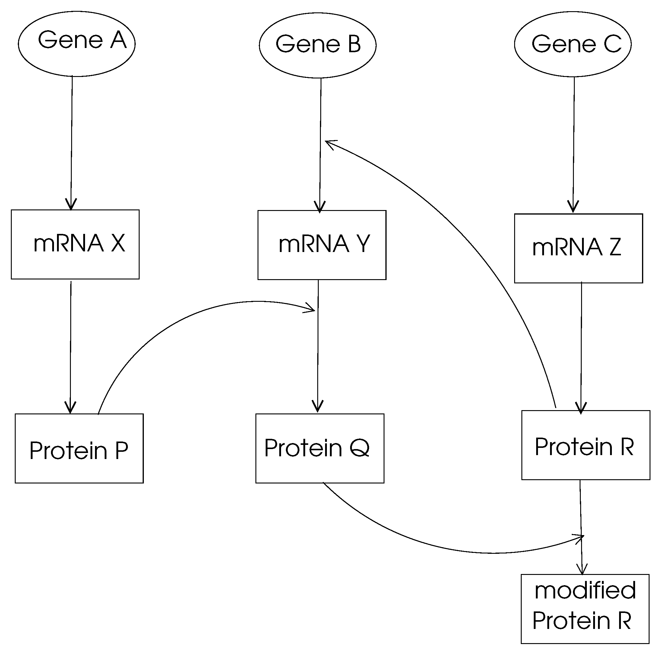
- Gene Regulation Networks: The main function of a gene in DNA is to provide the code to be used through transcription and translation processes to produce a protein. This process is called gene expression, and the mechanism of specific gene expression is controlled and affected by proteins that are coded by other genes, denoted regularity interactions. For example, gene X regulates gene Y if a change in the expression of gene X results in a change in the expression of gene Y. A gene regulation network (GRN) is made of genes, proteins, and various other molecules, and it may be modeled using a directed graph, with nodes representing these entities and the edges showing their biochemical interactions leading to regulations, as shown in Figure 2. Typically, a GRN is a sparse graph with small-world and power-law properties, which means there are only a few nodes that have very high out-degrees that regulate the expression of other genes. Moreover, the distance between any two nodes in a GRN network is small compared to the size of the network as being consistent with small-world properties.
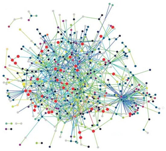 Figure 1. The PPI network of T. pallidum, taken from [6].Figure 1. The PPI network of T. pallidum, taken from [6].
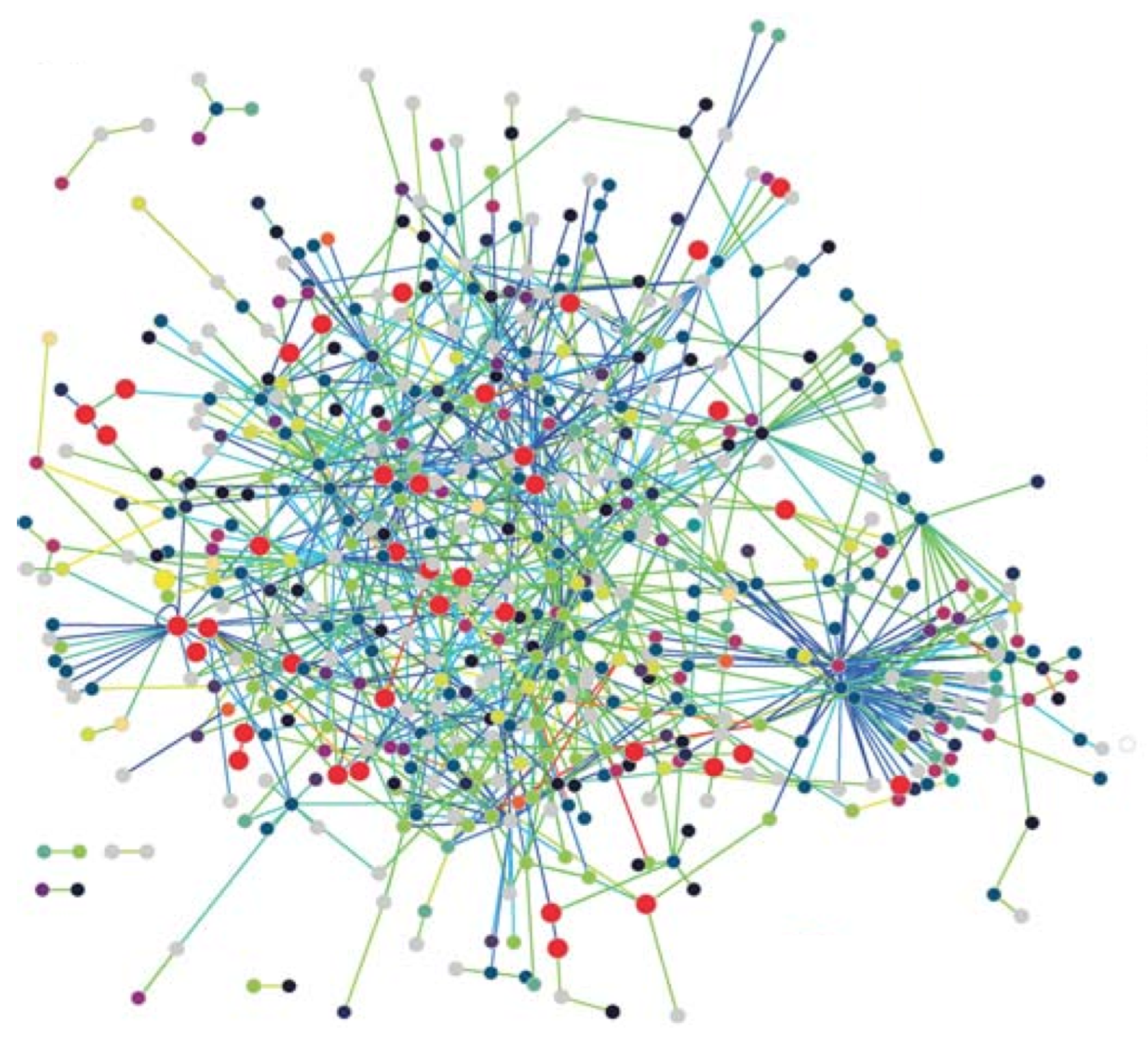
 Figure 2. A simple GRN.
 - Metabolic Pathways: The main ingredients of the cell, such as sugars, amino acids, and lipids, are produced by the basic chemical system called metabolism that works on ingredients called metabolites. The biochemical reactions in the cell that result in metabolisms can be modeled by directed or undirected graphs, with nodes representing metabolites and edges showing biochemical reactions that transform one metabolite to another one [7,8,9]. An edge in such a graph may also represent an enzyme that catalyzes a biochemical reaction. An undirected edge in the graph model denotes a reversible reaction where a directed edge means an irreversible one. A metabolic pathway is a sequence of biochemical reactions to perform a specific metabolic function. An example of a metabolic function is glycolysis, in which a glucose molecule is divided into two sugars that generate adenosine triphosphates (ATPs) to produce energy. Graphs representing metabolic pathways have the small-world and scale-free properties. A study of metabolic pathways may provide insight into pathogens causing infections in search of cures for diseases [10].
2.2. Networks outside the Cell
Biological networks outside the cell are of the following types.
- Brain Networks: We can analyze brain networks at the cell (neuron) level, or at a coarser functional level. A neuron in the brain fires when the sum of its input signal strengths exceeds a threshold. A neural network made of neurons performs various cognitive tasks such as problem solving, reasoning and, image processing. The artificial neural networks function similar to biological neural networks and have been used widely to implement various tasks in deep learning, which is a component of machine learning to be used for artificial intelligence tasks. At a coarser level, we can investigate the functions performed by the brain, using brain structural networks (BSNs) or brain functional networks (BFNs). A BSN basically reflects the structures of neural connections, whereas a BFN models the connnectedness of the functional regions of the brain. Studies of BFNs have shown that these networks are also small-world and scale-free networks, like most of the biological networks [11].
- Phylogenetic Networks: A phylogenetic tree shows evolutionary relationships among organisms, with leaves representing living organisms and the intermediate nodes, their common ancestors. A phylogenetic network is the general form of a phylogenetic tree where a node may have more than one parent.
- The Food Chain: Living organisms rely on food for survival. The food chain directed graph shows the relationships between the predators and the prey, where the direction of an edge is from the predator to the prey.
3. Large Graph Analysis
Large graphs representing biological networks can be analyzed using their local properties, focusing on nodes and their neighbors, or global properties that consider the network as a whole. We will investigate some useful local properties of large graphs to deduce their global properties in this section.
3.1. Degree Distribution
The degree distribution of a graph displays the percentage of vertices with a given degree, which may give an insight into the structure of the graph.
Definition 1
(degree distribution). The degree distribution of a given degree k in a graph G is the ratio of the number of vertices with degree k to the total number of vertices.
The degree distribution displays the probability of a randomly selected vertex to have a degree k. Formally,
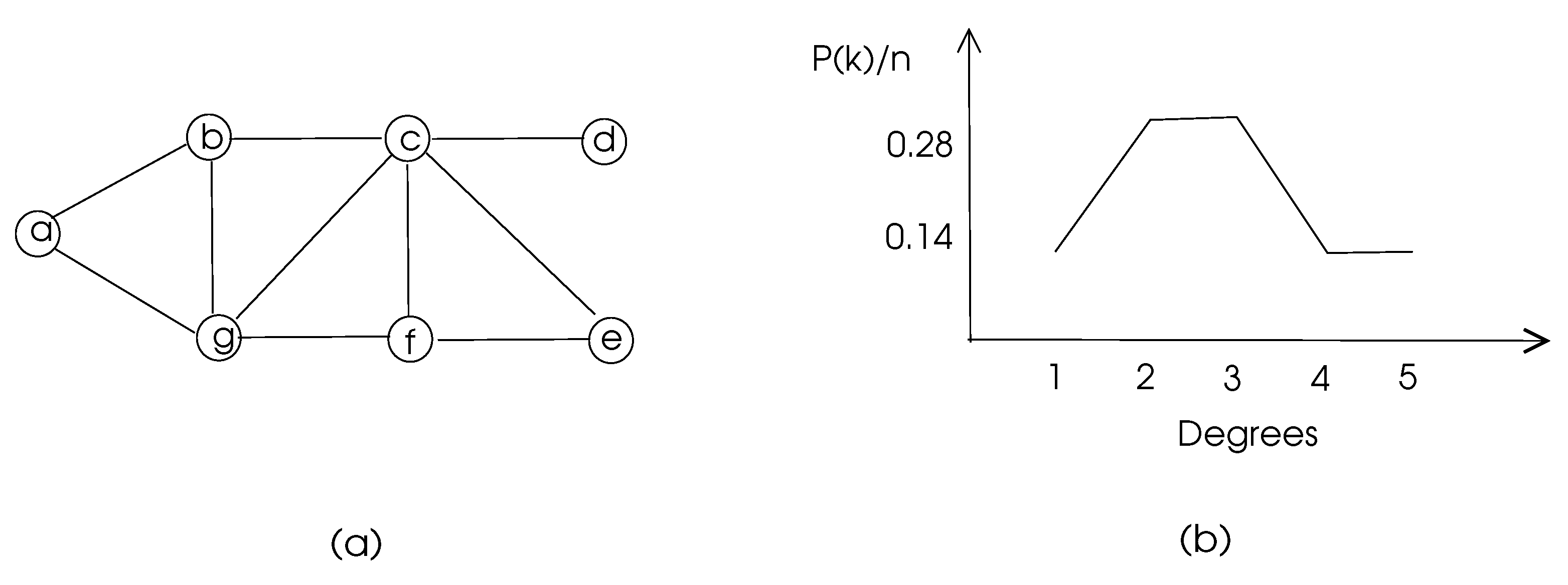
where is the number of vertices with degree k. The degree distribution of a sample graph is depicted in Figure 3.
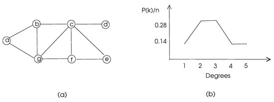
Figure 3.
Degree distribution of a sample graph with vertices a–g. (a) The graph. (b) Its degree distribution.
3.2. Density
The density of a graph provides general information about its structure; basically, it shows how well it is connected. Note that a sparse graph with few connections between its vertices may be represented by an adjacency list, whereas a dense graph is commonly represented by an adjacency matrix. There is no strict definition of a sparse or a dense graph; however, a general assumption is that the number of edges in a sparse graph grows as , whereas a dense graph has edges in the order of .
Definition 2
(graph density). The density of a graph G shown by is the ratio of the number of its edges to the maximum possible number of edges in G, as follows:
3.3. Clustering Coefficient
The clustering coefficient of a vertex in a graph displays how well its neighbors are connected. For example, a person with high clustering coefficient in a social network means having closely related friends for that person.
Definition 3
(clustering coefficient). The clustering coefficient of a node v is the ratio of the total number of edges between the neighbors of v to the maximum number of edges possible between these neighbors.
If k denotes the number of neighbors of a node v in a graph G, then the maximum possible number of edges connecting the vertices in the neighbor set of v is . Thus, the clustering coefficient of v can be expressed as below:
where r denotes the number of connections between the neighbor vertices of v. The average clustering coefficient of a graph G, , is calculated as the mean value of all of the clustering coefficients of nodes, as below:
The clustering coefficients of the nodes of the graph of Figure 3 are 1, 0.67, 0.5, 0, 1, 0.67, and 0.5, respectively, and the average clustering coefficient of this graph is 0.48.
3.4. Matching Index
The matching index of two nodes in a graph relates them by comparing their common neighbors with all of their neighbors. This parameter basically shows the similarity of two nodes in a graph; a high number of common neighbors means that these nodes have similar properties. As an example, two persons in a social network with many common friends may have similar personalities.
Definition 4
(matching index). The matching index of two nodes u and v in a graph is the ratio of the number of their common neighbors to the number of the union of all of their neighbors.
For example, nodes c and g in Figure 3 have two common neighbors b and f, and the total number of their neighbors is 6. Thus, the matching index of c and g is 0.33. In a biological network, a high matching index of two nodes may mean a similar functionality of these nodes.
3.5. Centrality
Centrality is yet another measure to determine the importance of nodes or edges in a complex network. This parameter is evaluated by calculating the shortest paths over the nodes.
3.5.1. Closeness Centrality
The closeness centrality of a node v in a graph is calculated by summing the distances from v to all the other nodes, and then taking the reciprocal of this sum, as shown below.
with showing the distance between vertices u and v. The distances in an unweighted graph may be found using the breadth-first-search algorithm, and the distances in a weighted graph may be calculated using Dijkstra’s shortest path algorithm or Bellman-Ford algorithm [4]. This parameter is used to determine how central a node in a graph is, since a node with a high closeness centrality means that node is close to all other nodes. The closeness centrality for node a in the graph of Figure 3 is 0.08, whereas node c has 0.14 for this parameter, which shows that c is more central than a, as can be visually detected.
3.5.2. Vertex Betweenness Centrality
The vertex betweenness centrality of a node v, , is used to determine the importance of node v in a graph by calculating the number of shortest paths through node v and dividing this number by the total number of shortest paths in the graph, as shown below.
where shows the number of shortest paths between all nodes s and t other than node v, and is the number of shortest paths through node v.
3.5.3. Edge Betweenness Centrality
Edge betweenness centrality is similar to vertex betweenness centrality, but the shortest paths through an edge are calculated instead of a vertex. This parameter may be used for clustering in biological networks, as we will see in the following sections. The edge betweeness of an edge e may be stated as below.
3.6. Topological Index
Chemical graph theory combines graph theory and chemistry, where graphs are used to model molecules. The physical properties of a graph are affected by its chemical structure, which may be represented by a graph. These properties may be modeled using topological indices, which are defined for the underlying chemical structure.
A biological network may be represented by a function that maps its network structure as represented by a graph G to a topological index, which is a positive real number. This parameter is a measure of the physical, chemical, and biological properties of the biological network. As an example, let us consider the eccentricity of a vertex v of a graph , defined by , which is the maximum distance of vertex v in the graph. The eccentric version of the geometric-arithmetic index, as the fourth geometric-arithmetic eccentricity index, may now be defined considering the eccentricities of all vertices in the graph, using the following formula [12]:
Various topological indices may be derived using the GA index [13]. Topological indices are widely used to analyze chemical graphs and to infer the functioning of chemical structures based on these indices. Some commonly used topological indices are as follows [14,15,16].
- The first Zagrep index
- The second Zagrep indexwhere is the degree of vertex v.
- The Wiener indexwhere is the distance as the number of edges between vertices u and v.
3.7. Network Perturbation Analysis
A perturbation of a biological system is the alteration or deviation of its functions, caused either by internal or external events. Molecular changes such as mutations may be the leading causes of perturbations in a biological network. Various studies address research on the prediction of perturbation, using the topology of the network [17], which may be used to predict the spread modeling of diseases to be used for treatment and drug development for diseases.
4. Large Network Models
An analysis of the topological properties of biological networks reveal that these networks have small diameters, allowing any node to be reached from any other node in only a few hops. Moreover, these networks have very few nodes with very high degrees called hubs, where the majority of nodes have low degrees. They can be classified as random networks, small-world networks, and scale-free networks, based on these properties.
- Random networks: These types of networks, proposed by Erdos and Renyi, assume that an edge between the vertices u and v is formed with the probability . The degree distribution in random networks is binomial, following a Poisson distribution. A random network has a short average path length and it has a clustering coefficient that is inversely proportional to the size of the network.
- Small-world networks: These types of networks are characterized by low average path lengths and short diameters. Biological networks such as PPI networks, GRNs, and metabolic pathways; and other complex networks such as social networks and the Internet exhibit this property. The diameter of a small-world network is proportional to , where n is the number of nodes in the network.
- Scale-free networks: Most biological networks have few high-degree nodes, with many low-degree ones. The PPI network of T. pallidum in Figure 1 exhibits small-world and scale-free network properties, as can be seen. These networks, along with various other complex networks, obey the power-law degree distribution shown by the following equation,where is known as the power-law exponent. These networks are called scale-free networks. The PPI networks of E. coli, D. melanogaster, C. elegans, and H. Pylori were shown to be scale-free. Barabasi and Albert provided a method to form a scale-free network with the following steps [18]:
- Growth: A new node is added to the network at each discrete time t.
- Preferential Attachment: A new node u is attached to any node v in the network with a probability proportional to the degree of v, which means that higher degree nodes tend to have more neighbors at each attachment.
- Hierarchical Networks: A study of biological networks shows that the clustering coefficients of nodes are inversely proportional to their degrees. This unexpected result means that lower degree nodes in these networks have higher clustering coefficients than the hubs. A hierarchical network model of a biological network captures all of the observed properties, such as small-world and scale-free, with an additional property that is exhibited by dense clusters of low-degree nodes, connected by high-degree hubs. That is, the neighbors of low-degree nodes in such networks are highly connected but the nodes around the high-degree nodes are sparsely connected.
5. Cluster Discovery in Biological Networks
Graph clustering aims at finding dense regions of a graph that have many connections among the nodes in that region. In the extreme case, this problem may be viewed as finding cliques of a graph, which is an NP-Hard problem. Finding clusters in biological networks may provide an insight into intense activities in these regions, to understand the health and disease states of organisms. The quality of the discovered clusters may be evaluated using its modularity Q of a detected cluster set , which is defined using the following formula [19,20]:
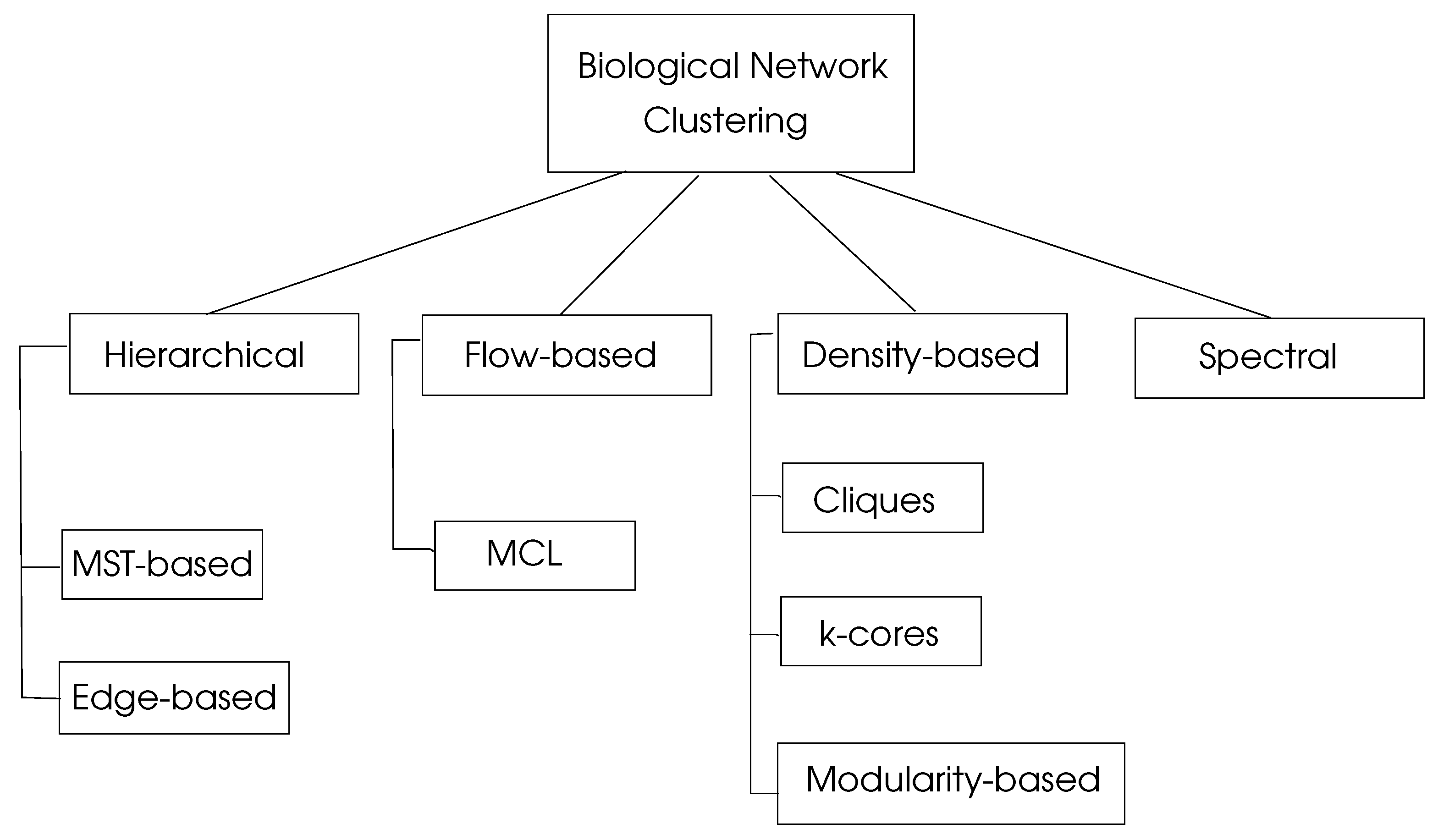
where are the percentages of the number of edges in , and is the percentage of edges with at least one edge in . This parameter shows the sum of the differences of probabilities of an edge being in and a random edge that would exist in with a maximum value of unity. Graph clustering algorithms may be classified into four basic types as hierarchical, density-based, flow-based, and spectral algorithms, as depicted in Figure 4.
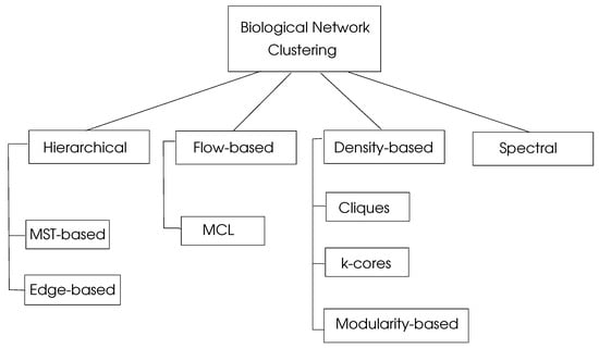
Figure 4.
Classification of biological network clustering algorithms, adapted from [4].
5.1. Hierarchical Clustering
Hierarchical clustering algorithms build clusters iteratively, commonly starting by initializing each vertex as a cluster and then merging close clusters to form new clusters at each step in agglomerative clustering. Alternatively, the whole graph may be considered as a cluster, and then the separation of remotely related regions provide clusters in divisive clustering. The distances between two clusters and that need to be calculated at each step can be defined as follows:
- Single Link: The distance between two closest points, with one of them in and other in , is considered.
- Complete Link: The distance between the two points in two clusters that are farthest is used.
- Average Link: The average distance between every pair of points in and is considered.
The output of a hierarchical clustering is a tree structure called a dendogram, which can be divided into the required number of clusters by drawing a horizontal line. Two main methods of hierarchical graph clustering in biological networks are the minimum spanning tree (MST)-based clustering and the edge betweenness-based clustering. The MST-based clustering assumes that an MST T of a weighted graph is constructed beforehand and that the heaviest edge is removed from T at each step to form clusters. The basic idea of this algorithm is to assume that the nodes that are far apart should be in different clusters. The removal of the heaviest edges are needed to form k clusters. Instead of removing a single edge at each iteration, edges that have weights that are larger than a threshold may be removed at each step, resulting in a number of edges being deleted from the MST. Then, the quality Q of the clusters may be assessed, and this process continues until a target quality is achieved. Clustering through MST in parallel (CLUMP) is an MST-based parallel clustering method that is designed to detect dense regions of biological data [21], and parallel MST construction algorithms are reviewed in [22].
The edge betweenness-based clustering method takes a similar approach by calculating the edge betweenness values of all edges in the graph and then removing the high valued edges to form clusters [23]. The basic idea in this algorithm is that the edges with the high betweenness values have a high probability of joining clusters, as many shortest paths run through them as a bridge in a graph. Yang and Lonardi provided a parallel implementation of this algorithm and showed that a linear speedup is achieved, with up to 32 processors [24].
5.2. Density-Based Clustering
In the extreme case, a clique of a graph is a perfect cluster, with every node being connected to every other node in this structure. Cliques in biological networks are rare, due to the dynamicity of these networks with frequent edge deletions; however, clique-like structures, which have less connections than cliques that still exhibit a dense region in a graph, may be sought in polynomial time.
Bron and Kerbosch provided a recursive backtracking algorithm [25] to find cliques of a graph with a time complexity off . A scalable parallel implementation of the Bron and Kerbosch algorithm on a Cray XT supercomputer was reported in [26]. Mohseni-Zadeh et al. provided an algorithm to cluster protein sequences using the extraction of maximal cliques [27], and Jaber et al. proposed a parallel version of this algorithm using Message Passing Interface [28].
A k-core of a graph G is a subgraph of G, with each vertex in having a minimum degree of k. Thus, finding the k-cores of a graph may provide dense regions which are clusters of the graph. Batagelj and Zaversnik provided an algorithm that finds k-cores in time in a connected graph [29]. The Molecular Complex Detection (MCODE) Algorithm based on k-cores is used to detect protein complexes in large PPI networks [30], and a distributed k-core algorithm for large networks is proposed in [31].
Girvan and Newman proposed a modularity-based algorithm that works iteratively by considering each node of the graph as a cluster initially, and then joining two clusters that will increase the modularity parameter Q best. The algorithm stops when any merge operation decreases the Q parameter [20]. A modularity-based distributed clustering algorithm was proposed by Gehweiler et al. [32], and Reidy et al. provided a scalable parallel modularity-based clustering algorithm for social networks [33].
5.3. Flow-Based Clustering
Flow-based clustering algorithms make use of the water distribution network model, in which the pumped water will be collected at storage points with many pipe connections. The nodes of the graph correspond to storage places, and the edges represent the pipes in this model. Markov Clustering Algorithm takes this approach by considering random walks from a node u, and assuming that such a walk will end in the same cluster as the node u [34]. Thus, this method finds the collection points of random walks to detect clusters. This algorithm is successfully used to find clusters in biological networks [35,36], and parallel versions of the Markov Clustering Algorithm are presented in [37,38].
5.4. Spectral Clustering
Spectral clustering algorithms use the algebraic properties of a graph to detect dense regions in the graph. The Laplacian matrix of a graph is defined as , where D is a diagonal matrix with each diagonal element denoting the degree of vertex i, and A is its adjacency matrix. In normalized form, . The eigenvalues of L are real, since L is real and symmetric. The second eigenvalue, called the Fiedler value, and its eigenvector, called the Fiedler vector F [39], can be used to form clusters of the graph G, as follows. Spectral bisection algorithms work by testing each entry , and if it is larger than a constant value, commonly 0, it is placed in one cluster; otherwise, in the other cluster. This algorithm may be invoked recursively to find any required number of clusters. A parallel version of the spectral clustering algorithm was proposed by Chen et al. [40].
5.5. Fuzzy Clustering
Fuzzy clustering is a fundamental method of grouping objects such that an object may belong to more than one cluster. In other words, clusters may overlap in this type of clustering. This method is commonly applied for clustering data points in applications such as image segmentation, pattern recognition, and medical diagnosis. The main advantages of this approach are its flexibility in dealing with complex data structures when it may not be easy to determine their clusters using traditional methods, and its robustness to outliers, since a gradual transition from one cluster to another may be performed. However, fuzzy clustering algorithms may be more complex than their counterparts, as optimization over membership to multiple clusters should be considered.
Data points are distributed to random clusters of predetermined number as the first step of this method. Then, centroids for each cluster are computed, followed by the evaluation of each point to the centroid of its cluster. The membership values are then updated based on these distances, and this process is repeated until stable membership values are obtained.
Fuzzy clustering is basically defined and implemented for data points; however, it may also be implemented in complex networks, providing the incorporation of link and node attributes while clustering. The Fuzzy Clustering Algorithm for Complex Networks (FCAN) [41] is proposed to detect clusters in a complex network by evaluating the content relevance and the link structure at the same time. The content similarity of two nodes provides a measure of their probability of being members of the same cluster. Moreover, the link structure data are used, together with node similarity information by a maximization optimization procedure to identify the clusters of a node. The authors show a successful implementation of FCAN in social networks to identify the clusters in this study. An Improved Fuzzy-based Graph Clustering Algorithm for Complex Networks with Multi-objective Particle Swarm Optimization (FCAN-MOBSO) [42] is an enhanced version of the FCAN algorithm, aiming to eliminate the improper regularization design and slow convergence disadvantages of FCAN. This algorithm uses multi-objective particle swarm optimization (MOBSO) to achieve a significantly increased convergence rate via the adoption of an instance-frequency-weighted regularization method to handle unbalanced cluster memberships. Moreover, it decomposes the optimization problem to a set of sub-optimization problems and provides a solution via consensus, using OBSO among these problems. The authors show that this method provides improved cluster quality and faster convergence compared to FCAN when applied to citation and social networks.
6. Network Motifs
A network motif is a frequently repeating subgraph in a graph which represents a biological network. A motif with high occurrences may indicate a basic function that is carried out by that motif in the network, which may lead to the determination of the function performed. Moreover, discovering similar motifs in two or more organisms may provide insight into their genetic affinity, and thus, into the evolutionary process. Unfortunately, the detection of a subgraph with a given number of nodes in a graph is an NP-Hard problem, which means that heuristic solutions are the only possible choices in most cases.
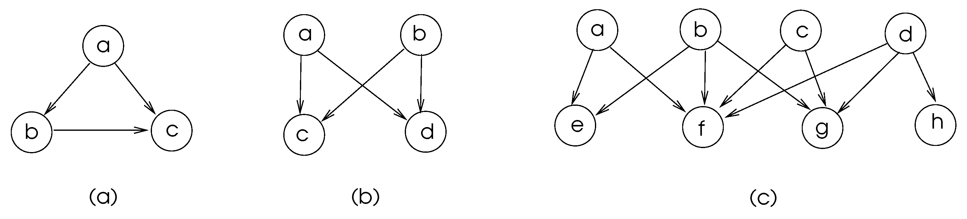
Some commonly found motifs in biological networks are depicted in Figure 5. The motifs in (a) and (b) of this figure are frequent in transcriptional regulatory networks and neuronal connectivity networks [4]. The feed-forward-loop ensures that the signal sent from node a is delivered to node c, and node c discards the second arrival of a signal from node a, which shows that there is some level of fault tolerance in these network structures.
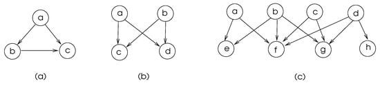
Figure 5.
Commonly found biological network motifs with vertices a–h. (a) Feed-Forward-Loop, (b) Bifan, (c) Multi-input motifs.
6.1. Motif Discovery
There exist two basic methods of motif search in a biological network; all subgraphs of given order k are searched in a network-centric motif search; alternatively, a distinct motif may be searched in G in the motif-centric method. The following steps are commonly performed to discover a motif of order k in a graph G representing a biological network.
- The detection of in G may be performed via exact counting, which involves the enumeration of all subgraphs of order k. This method evidently has a high time complexity; alternatively, sampling-based methods that work in a representative sample of the graph may provide approximate solutions.
- Isomorphic classes of the discovered motifs should be determined, since various motifs may be isomorphic to each other.
- Statistical significance of the discovered motifs in G should be determined. Commonly, a similar structured set of random graphs are generated, and motifs are searched in these graphs. If the motifs found in G are statistically higher in number than the ones found in the graphs of set , we can conclude that they do represent some biological function in the network represented by G.
6.2. Background
Finding the motifs in a graph is closely related to the graph isomorphism problem. Two graphs, and , are isomorphic if there is a one-to-one relationship, (English Editor: Please check that intended meaning is retained.) and onto function , such that . The number of motifs found in a graph is called its frequency, which can be evaluated in three different ways, denoted by , , and . is computed by discovering all the motifs of a given size with overlapping nodes and edges, whereas shows edge disjoint motifs with node overlaps only, and the frequency shows the number of edge and vertex disjoint motifs.
The goodness of a motif search algorithm is commonly decided by generating a set of n random graphs, applying the algorithm on these graphs, and comparing the results via statistical evaluation. Three statistical methods to evaluate a motif discovery algorithm are as follows.
- P-value: This parameter is calculated by finding the number of elements of the randomly generated set that have a greater frequency of motif m than in the target graph G. A motif m is considered a significant motif if P-value of m, , given below, is less than 0.01.where is 1 if the occurrence of motif m in the random network is higher, and 0 if it is lower than that found in the target graph G.
- Z-score: The Z-score of a motif m, , in a graph G, is evaluated using the following formula:where is the number of discovered motifs m in G, and and are the mean and variance frequencies of m in a set of random networks. A motif m is significant if [43].
- Motif significance profile: The motif significance profile vector SP is structured with elements as Z-scores of motifs , and normalized to unity as below. Various graphs may then be compared for any common motifs contained in them.
6.3. Review of Motif Searching Algorithms
There is significant research on motif searching algorithms, which can be viewed as network centric and motif centric, as shown in Figure 6. Exact census refers to the exact numbering of motifs, whereas sampling methods work by selecting a representative sample of the network under consideration and then projecting the computed results to the whole network.
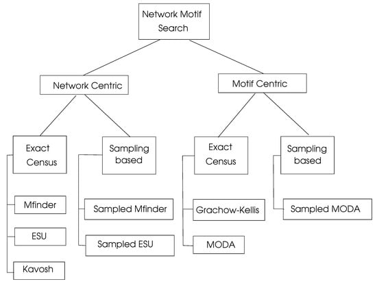
Figure 6.
Network motif search algorithms, adapted from [4].
6.3.1. Network Centric Search Algorithms
, proposed by Milo et al. [43] uses the frequency concept and can be applied to both directed and undirected graphs. It starts with an edge in the target graph G and enumerates all subgraphs of order k that contain . Due to its high memory space requirement and high run-time, it can be used only up to a motif size of five. The sampled version of , called Edge Sampling Algorithm (ESA), selects an edge and its adjacent edges randomly to form a motif of size k [44].
Enumerate Subgraph (ESU) Algorithm [45,46] is an efficient motif search algorithm implemented using both exact census and sampling-based approaches. The randomized version of this algorithm (RAND-ESU) was compared with the algorithm in finding motifs of the transcriptional network of E. coli [47], the transcriptional network of S. cereviciae [48], the neuronal network of Caenorhabditis elegans [44], and the food web of the YTHAN estuary [49]. The authors concluded that RAND-ESU has a much better performance than the sampling-based for graphs with sizes of larger than five. , which consists of steps enumeration, classification, random graph generation, and motif identification, is a network motif discovery tool designed for directed and undirected graphs [50].
6.3.2. Motif Centric Search Algorithms
These algorithms may input a single motif structure or simply the size k of a motif to search. They are commonly used in cases when k or the structure of a motif is known before the search. Grachow-Kellis algorithm uses a symmetry breaking method to prevent subgraph isomorphism tests, which results in better performance when compared to other algorithms [51]. This algorithm was implemented in a PPI network [52] and a transcription network of S. cerevisiae [53], and was compared with other methods of motif discovery. It was shown that the Grachow-Kellis algorithm provides an exponential time improvement compared to Mfinder when subgraphs up to size 7 are considered. MODA is a motif search algorithm that uses the expansion tree approach to employ previously searched queries [54]. The sampling version of MODA provides faster motif searches by sampling nodes with probabilities related to their degrees [54].
6.3.3. Parallel Motif Search Algorithms
As the motif search problem is time consuming in general, various studies aim to parallelize this process. The three steps of motif finding are subgraph enumeration, detecting subgraph isomorphisms, and evaluating statistical significance as outlined, and there is potential at each step for parallel processing. The graph under consideration may be partitioned, and the first two steps may be carried in these partitions, considering border vertices carefully. The third step can be conveniently performed in parallel by assigning elements of the randomly generated graph set to the processors.
Parallel exact motif discovery is performed by searching the motifs in the neighborhoods of nodes in parallel in [55], and a distributed version of the Grochow–Kellis algorithm via query parallelization and network partitioning is presented in [56]. A parallel version of a motif centric algorithm that attempts to find a set of input motifs instead of a single one was proposed in [57], and a parallelized version of the ESU algorithm was presented in [58]. An extended and generalized parallel motif search based on the ESU algorithm is presented in [59]. Recently, Ruzgar et al. provided an efficient parallelization of the ESU algorithm [60], and a more recent review of network motif search algorithms can be found in [61].
7. Network Alignment
Network alignment aims at finding similarities between two or more biological networks, which helps to deduce the phylogenetic relationships between them to predict future organism structures, and also to investigate the evolutionary process. Moreover, finding conserved regions in two or more organisms may indicate shared functional modules within them. Global alignment methods compare two or more networks as a whole, whereas local alignment procedures attempt to find similar subgraphs in the graphs representing the networks. The pairwise alignment is between two networks, and multiple alignment is performed over a set of networks. Comparing biological networks of diverse organisms using global alignment is not usually preferred; the local alignment is the reasonable choice, since global similarities would be minimal in these cases.
7.1. Background
Subgraph isomorphism is the process of searching for a smaller graph in a larger graph with the maximal size that is isomorphic to the smaller graph. Network alignment is the more general form of subgraph isomorphism in which we search for a set of subgraphs in the larger graph; thus, this process is NP-Hard as the subgraph isomorphism problem, which means approximation algorithms, or more frequently, heuristic algorithms are commonly used for this purpose.
A matching of a graph is defined as a subset of its disjoint edges, in other words, these edges do not share any endpoints. A maximal matching of an unweighted graph G can not be embedded in any other matching of the graph and a maximum matching (MaxM) of an unweighted graph G has the maximum size among all matchings of G. When a graph G is weighted, MM and MaxM of G is its matchings with the maximal and maximum weights of G, respectively. We can use the maximal weighted matching of a complete bipartite graph for network alignment with the following reasoning. Let a bipartite graph represent two networks, with as the nodes of the first network and as the nodes of the second network . Let us further assign weights proportional to the similarities of nodes to the edges of between and . Then, a maximal weighted matching in G will exhibit how similar these two networks and are. The main steps in a global network alignment algorithm based on this approach may be stated as follows.
- Form the similarity matrix R with entry showing the similarity score of the nodes and in input networks and , respectively.
- Implement a weighted matching algorithm to assess the similarity of the networks and .
7.2. Alignment Quality
The topological similarity of two networks displays the similarity of the structures that they exhibit, whereas node similarity is a measure of the affinity of the node structures; for example, the amino acid sequence in a protein node of a PPI network. The edge correctness (EC) parameter shown below is one measure of similarity between two graphs, to [62].
with f as an edge mapping function from graph to . This parameter evaluates the correctness of the alignment by testing the percentage of the correctly aligned edges. The induced conserved structure (ICS) is based on EC attempts to map the sparse regions or the dense regions of the two graphs [63]. The size of the largest connected component (LCC) shared by the input graphs is another parameter to estimate the similarity of two graphs, with a larger LCC exhibiting a greater similarity. As with the network motif search algorithms, a random set of graphs may be generated, and the quality of the alignment of two input graphs may be compared with these random networks statistically [64]. We can now classify network alignment algorithms as being pairwise or multiple, or local or global, and using node and/or topological similarity. Frequently, node and topological similarity are both used with assigned weights to each method. In PPI networks, node similarity may be evaluated using biological sequence alignment tools such as the Basic Local Alignment Search Tool (BLAST) [65].
7.3. Review of Network Alignment Algorithms
The PathBLAST tool provides network alignment for PPI networks to discover protein pathways and complexes [66]. The IsoRank algorithm, based on the PageRank algorithm, finds global network alignment between two PPI networks using both node similarity and local connectivity structure [62]. The maximum-weight-induced subgraph (MaWIsh) is a pairwise local alignment algorithm for PPI networks [67]. Natalie [68] is a tool for pairwise global network alignment and uses the Lagrangian relaxation method proposed by Klau [69]. A global alignment algorithm, Graph Aligner (GRAAL), uses topological data to discover the similarity of networks [70]. Scalable Protein Interaction Network Alignment (SPINAL) is a two-phase global alignment algorithm with coarse-grained alignment in the first phase and a fine-grained alignment in the second [71].
The two main steps of network alignment are the formation of the similarity matrix R and then the maximal weighted matching step. A simple algorithm for this task picks the heaviest edge incident at a randomly selected node and deletes the node and all adjacent edges at each step until no more edges are left [72], with a time complexity of and an approximation ratio of 0.5. A distributed version of this algorithm [73] and then its parallel version was proposed in [74]. A parallel maximal weighted matching algorithm based on auctions was proposed in [75], and a recent study found the weighted matching of a bipartite graph by partitioning the adjacency matrix of the graph to processors with significant speedups [76], and a survey of network alignment methods is provided in [77].
8. Discussion
Graph theory is a rich and dynamic branch of mathematics studied extensively by researchers with numerous results, both theoretically and with discovered algorithms applied to many diverse applications. Biological networks can be represented using graphs, and the analysis of these networks can be performed conveniently using the results of graph theory. In this survey, we outlined basic large graph analysis methods, classified large biological networks, and turned our attention to three main problems in the analysis of biological networks, which are clustering, network motif search, and network alignment. All of these problems are NP-Hard, defying solutions in polynomial time, which means that approximation algorithms or suitable heuristics are the only solutions in most cases.
Graph clustering aims at finding closely related regions of graphs representing biological networks, and these zones may indicate high activities and sometimes the disease states of an organism. Data and graph clustering remains one of the most highly studied topics in Computer Science and various other disciplines such as Statistics. We reviewed the basic methods of clustering as hierarchical, dense, spectral, and fuzzy clustering. Network motif search identifies repeating subgraphs in a graph of a biological network to investigate the functions performed by these subgraphs. We reviewed basic approaches and algorithms that aim for efficient motif search, globally or locally. Network alignment, which is addressed by various researchers, is another basic problem in biological networks targeting to find similarities between networks to detect the basic functions performed by them, and to deduce ancestral relationships.
Although there are various algorithms and methods for these three distinct problems, efficient implementations are required due to the large size of the biological networks. A basic approach for effective algorithms for this purpose is to parallelize the steps of the sequential algorithms. In network motif search, we described ways of the parallel implementation steps, namely, the detection of a motif, finding its isomorphic class, and evaluating the statistical significance of the results. The two main steps of network alignment, which are forming the similarity matrix and applying maximal weighted matching in this matrix, can also be performed in parallel. Algebraic graph analysis is the method of analyzing the algebraic properties of graph matrices and deducing graph structures using these results. This approach is relatively more recent than classical graph analysis, and may be conveniently used in various applications, since parallel matrix operations are already available. Basic algebraic graph algorithms using Python are reviewed in [78]. In summary, it is expected that graph clustering, network motif search, and network alignment will be three important areas of research in the graph-theoretical analysis of biological networks.
Funding
This research received no external funding.
Informed Consent Statement
Not applicable.
Conflicts of Interest
The author declares no conflict of interest.
References
- Vogelstein, B.; Lane, D.; Levine, A. Surfing the p53 network. Nature 2000, 408, 307–310. [Google Scholar] [CrossRef]
- Carbonell, P.; Anne-Galle Planson, A.-G.; Davide Fichera, D.; Jean-Loup Faulon, J.-P. A retrosynthetic biology approach to metabolic pathway design for therapeutic production. BMC Syst. Biol. 2011, 5, 122. [Google Scholar] [CrossRef]
- Mason, O.; Verwoerd, M. Graph theory and networks in biology. IET Syst. Biol. 2007, 1, 89–119. [Google Scholar] [CrossRef]
- Erciyes, K. Distributed and Sequential Algorithms for Bioinformatics; Springer Computational Biology Series; Springer: Basel, Switzerland, 2013; Chapter 7 and Chapters 10–13. [Google Scholar]
- Jeong, H.; Mason, S.P.; Barabási, A.-L.; Oltvai, Z.N. Lethality and centrality in protein networks. Nature 2011, 411, 41–42. [Google Scholar] [CrossRef]
- Titz, B.; Rajagopala, S.V.; Goll, J.; Hauser, R.; McKevitt, M.T.; Palzkill, T.; Uetz, P. The binary protein interactome of Treponema pallidum, the syphilis spirochete. PLoS ONE 2008, 3, e2292. [Google Scholar] [CrossRef]
- He, Y.; Chen, Z.; Evans, A. Structural insights into aberrant topological patterns of large scale cortical networks in Alzheimers disease. J. Neurosci. 2008, 28, 4756–4766. [Google Scholar] [CrossRef]
- Schuster, S.; Fell, D.A.; Dandekar, T. A general definition of metabolic pathways useful for systematic organization and analysis of complex metabolic networks. Nat. Biotechnol. 2000, 18, 326–332. [Google Scholar] [CrossRef]
- Vidal, M.; Cusick, M.E.; Barabasi, A.L. Interactome networks and human disease. Cell 2011, 144, 986–998. [Google Scholar] [CrossRef]
- Junker, B. Analysis of Biological Networks; Wiley: Hoboken, NJ, USA, 2008; Chapter 9. [Google Scholar]
- Sporns, O. Networks of the Brain; MIT Press: Cambridge, MA, USA, 2016. [Google Scholar]
- Ghorbani, M.; Khaki, A. A note on the fourth version of geometric-arithmetic index. Optoelectron. Adv. Mater. Rapid Commun. 2010, 4, 2212–2215. [Google Scholar]
- Gao, W.; Wu, H.; Siddiqui, M.K.; Baig, A.Q. Study of biological networks using graph theory. Saudi J. Biol. Sci. 2018, 25, 1212–1219. [Google Scholar] [CrossRef]
- Basavanagoud, B.; Barang, A.P. M-polynomial of some cactus chains and their topological indices. Open J. Discret. Appl. Math. 2019, 2, 59–67. [Google Scholar] [CrossRef]
- Dobrynin, A.A.; Estaji, E. Wiener index of hexago- nal chains under some transformations. Open J. Discret. Math. 2020, 3, 28–36. [Google Scholar] [CrossRef]
- Zhang, X.; Saleem, U.; Waheed, M.; Jamil, M.K.; Zeeshan, M. Comparative study of five topological invariants of supramolecular chain of different complexes of N-salicylidene-L-valine. AIMS Math. Biosci. Eng. 2023, 20, 11528–11544. [Google Scholar] [CrossRef]
- Santolini, M.; Barabási, A.L. Predicting perturbation patterns from the topology of biological networks. Proc. Natl. Acad. Sci. USA 2018, 115, E6375–E6383. [Google Scholar] [CrossRef]
- Albert, R.; Barabasi, A. The statistical mechanics of complex networks. Rev. Mod. Phys. 2002, 74, 47–97. [Google Scholar] [CrossRef]
- Newman, M.E.J. Fast algorithm for detecting community structure in networks. Phys. Rev. E 2004, 69, 066133. [Google Scholar] [CrossRef]
- Newman, M.E.J.; Girvan, M. Finding and evaluating community structure in networks. Phys. Rev. E 2004, 69, 026113. [Google Scholar] [CrossRef]
- Olman, V.; Mao, F.; Wu, H.; Xu, Y. Parallel clustering algorithm for large data sets with applications in bioinformatics. IEEE/ACM Trans. Comput. Biol. Bioinform. 2009, 6, 344–352. [Google Scholar] [CrossRef]
- Murtagh, F. Clustering in massive data sets. In Handbook of Massive Data Sets; Springer: Berlin/Heidelberg, Germany, 2002; pp. 501–543. [Google Scholar]
- Girvan, M.; Newman, M.E.J. Community structure in social and biological networks. Proc. Natl. Acad. Sci. USA 2002, 99, 7821–7826. [Google Scholar] [CrossRef]
- Yang, Q.; Lonardi, S. A parallel edge-betweenness clustering tool for protein-protein interaction networks. Int. J. Data Min. Bioinform. (IJDMB) 2007, 1, 241–247. [Google Scholar] [CrossRef]
- Bron, C.; Kerbosch, J. Algorithm 457: Finding all cliques of an undirected graph. Commun. ACM 1973, 16, 575–577. [Google Scholar] [CrossRef]
- Schmidt, M.C.; Samatova, N.F.; Thomas, K.; Park, B.-H. A scalable, parallel algorithm for maximal clique enumeration. J. Parallel Distrib. Comput. 2009, 69, 417–428. [Google Scholar] [CrossRef]
- Mohseni-Zadeh, S.; Brezelec, P.; Risler, J.L. Cluster-C, an algorithm for the large-scale clustering of protein sequences based on the extraction of maximal cliques. Comput. Biol. Chem. 2004, 28, 211–218. [Google Scholar] [CrossRef]
- Jaber, K.; Rashid, N.A.; Abdullah, R. The parallel maximal cliques algorithm for protein sequence clustering. Am. J. Appl. Sci. 2009, 6, 1368–1372. [Google Scholar] [CrossRef]
- Batagelj, V.; Zaversnik, M. An O(m) algorithm for cores decomposition of networks. arXiv 2003, arXiv:0310049. [Google Scholar]
- Bader, G.D.; Hogue, C.W.V. An automated method for finding molecular complexes in large protein interaction networks. BMC Bioinform. 2003, 4, 2. [Google Scholar] [CrossRef] [PubMed]
- Montresor, A.; Pellegrini, F.D.; Miorandi, D. Distributed k-Core decomposition. IEEE Trans. Parallel Distrib. Syst. 2013, 24, 288–300. [Google Scholar] [CrossRef]
- Gehweiler, J.; Meyerhenke, H. A distributed diffusive heuristic for clustering a virtual P2P supercomputer. In Proceedings of the 7th High-Performance Grid Computing Workshop (HGCW10) in Conjunction with 24th International Parallel and Distributed Processing Symposium (IPDPS10), Atlanta, GA, USA, 19–23 April 2010. [Google Scholar]
- Riedy, J.; Bader, D.A.; Meyerhenke, H. Scalable multi-threaded community detection in social networks. In Proceedings of the IEEE 26th International Parallel and Distributed Processing Symposium Workshops and PhD Forum (IPDPSW), Shanghai, China, 21–25 May 2012; pp. 1619–1628. [Google Scholar]
- Dongen, S.V. Graph Clustering by Flow Simulation. Ph.D. Thesis, University of Utrecht, Utrecht, The Netherlands, 2000. [Google Scholar]
- Brohee, S.; van Helden, J. Evaluation of clustering algorithms for protein-protein interaction networks. BMC Bioinform. 2006, 7, 488. [Google Scholar] [CrossRef]
- Vlasblom, J.; Wodak, S.J. Markov clustering versus affinity propagation for the partitioning of protein interaction graphs. BMC Bioinform. 2009, 10, 99. [Google Scholar] [CrossRef]
- Bustamam, A.; Sehgal, M.S.; Hamilton, N.; Wong, S.; Ragan, M.A.; Burrage, K. An efficient parallel implementation of Markov clustering algorithm for large-scale protein-protein interaction networks that uses MPI. In Proceedings of the fifth IMT-GT International Conference Mathematics, Statistics, and Their Applications (ICMSA), Sumatra Barat, Indonesia, 9–11 June 2009; pp. 94–101. [Google Scholar]
- Bustamam, A.; Burrage, K.; Hamilton, N.A. Fast parallel Markov clustering in bioinformatics using massively parallel computing on GPU with CUDA and ELLPACK-R sparse format. IEEE/ACM Trans. Comp. Biol. Bioinform. 2011, 9, 679–691. [Google Scholar] [CrossRef]
- Fiedler, M. Laplacian of graphs and algebraic connectivity. Comb. Graph Theory 1989, 25, 57–70. [Google Scholar] [CrossRef]
- Chen, W.-Y.; Song, Y.; Bai, H.; Lin, C.-J.; Chang, E.Y. Parallel spectral clustering in distributed systems. IEEE Trans. Pattern. Anal. Mach. Intell. 2010, 33, 568–586. [Google Scholar] [CrossRef] [PubMed]
- Hu, L.; Chan, K.C. Fuzzy clustering in a complex network based on content relevance and link structures. IEEE Trans. Fuzzy Syst. 2015, 24, 456–470. [Google Scholar] [CrossRef]
- Hu, L.; Yang, Y.; Tang, Z.; He, Y.; XLuo, X. FCAN-MOPSO: An Improved Fuzzy-based Graph Clustering Algorithm for Complex Networks with Multi-objective Particle Swarm Optimization. IEEE Trans. Fuzzy Syst. 2023. [Google Scholar] [CrossRef]
- Kashtan, N.; Itzkovitz, S.; Milo, R.; Alon, U. Mfinder Tool Guide; Technical Report; Department of Molecular Cell Biology and Computer Science and Applied Mathematics, Weizman Institute of Science: Rehovot, Israel, 2002. [Google Scholar]
- Kashtan, N.; Itzkovitz, S.; Milo, R.; Alon, U. Efficient sampling algorithm for estimating sub-graph concentrations and detecting network motifs. Bioinformatics 2004, 20, 1746–1758. [Google Scholar] [CrossRef]
- Wernicke, S. Efficient detection of network motifs. IEEE/ACM Trans. Comput. Biol. Bioinform. 2006, 3, 347–359. [Google Scholar] [CrossRef]
- Wernicke, S.; Rasche, F. FANMOD: A tool for fast network motif detection. Bioinformatics 2006, 22, 1152–1153. [Google Scholar] [CrossRef]
- Shen-Orr, S.S.; Milo, R.; Mangan, S.; Alon, U. Network motifs in the transcriptional regulation network of Escherichia Coli. Nat. Gen. 2002, 31, 64–68. [Google Scholar] [CrossRef]
- Milo, R.; Shen-Orr, S.; Itzkovitz, S.; Kashtan, N.; Chklovskii, D.; Alon, U. Network motifs: Simple building blocks of complex networks. Science 2004, 298, 824–827. [Google Scholar] [CrossRef]
- Williams, R.J.; Martinez, N.D. Simple rules yield complex food webs. Nature 2000, 404, 180–183. [Google Scholar] [CrossRef]
- Kashani, Z.R.; Ahrabian, H.; Elahi, E.; Nowzari-Dalini, A.; Ansari, E.S.; Asadi, S.; Mohammadi, S.; Schreiber, F.; Masoudi-Nejad, A. Kavosh: A new algorithm for finding network motifs. BMC Bioinform. 2009, 10, 318. [Google Scholar] [CrossRef] [PubMed]
- Grochow, J.; Kellis, M. Network motif discovery using subgraph enumeration and symmetry-breaking. In Proceedings of the 11th Annual International Conference Research in Computational Molecular Biology (RECOMB’07), Oakland, CA, USA, 21–25 April 2007; pp. 92–106. [Google Scholar]
- Han, J.-D.J.; Bertin, N.; Hao, T.; Goldberg, D.S.; Berriz, G.F.; Zhang, L.V.; Dupuy, D.; Walhout, A.J.M.; Cusick, M.E.; Roth, F.P.; et al. Evidence for dynamically organized modularity in the yeast protein-protein interaction network. Nature 2004, 430, 88–93. [Google Scholar] [CrossRef] [PubMed]
- Costanzo, M.C.; Crawford, M.E.; Hirschman, J.E.; Kranz, J.E.; Olsen, P.; Robertson, L.S.; Skrzypek, M.S.; Braun, B.R.; Hopkins, K.L.; Kondu, P.; et al. Ypd(tm), pombepd(tm), and wormpd(tm): Model organism volumes of the bioknowledge(tm) library, an integrated resource for protein information. Nucleic Acids Res. 2001, 29, 75–79. [Google Scholar] [CrossRef]
- Omidi, S.; Schreiber, F.; Masoudi-Nejad, A. MODA: An efficient algorithm for network motif discovery in biological networks. Genes Genet. Syst. 2009, 84, 385–395. [Google Scholar] [CrossRef] [PubMed]
- Wang, T.; Touchman, J.W.; Zhang, W.; Suh, E.B.; Xue, G. A parallel algorithm for extracting transcription regulatory network motifs. In Proceedings of the IEEE International Symposium on Bioinformatics and Bioengineering, Minneapolis, MN, USA, 19–21 October 2005; IEEE Computer Society Press: Washington, DC, USA, 2005; pp. 193–200. [Google Scholar]
- Schatz, M.; Cooper-Balis, E.; Bazinet, A. Parallel Network Motif Finding; Technical Report; University of Maryland Insitute for Advanced Computer Studies: College Park, MD, USA, 2008. [Google Scholar]
- Ribeiro, P. Efficient and Scalable Algorithms for Network Motifs Discovery. Ph.D. Thesis, Doctoral Programme in Computer Science, Faculty of Science of the University of Porto, Porto, Portugal, 2009. [Google Scholar]
- Ribeiro, P.; Silva, F.; Lopes, L. A parallel algorithm for counting subgraphs in complex networks. In Proceedings of the 3rd International Conference on Biomedical Engineering Systems and Technologies, Valencia, Spain, 20–23 January 2010; pp. 380–393. [Google Scholar]
- Ribeiro, P.; Silva, F.; Lopes, L. Parallel discovery of network motifs. J. Parallel Distrib. Comput. 2012, 72, 144–154. [Google Scholar] [CrossRef]
- Ruzgar, E.; Erciyes, K.; Dalkilic, M.E. Parallelization of network motif discovery using star contraction. Parallel Comput. 2021, 101, 102734. [Google Scholar]
- Patra, S.; Mohapatra, A. Review of tools and algorithms for network motif discovery in biological networks. IET Syst. Biol. 2020, 14, 171–189. [Google Scholar] [CrossRef]
- Singh, R.; Xu, J.; Berger, B. Pairwise global alignment of protein interaction networks by matching neighbourhood topology. In Research in Computational Molecular Biology, Proceedings of the 11th Annunal International Conference, RECOMB 2007, Oakland, CA, USA, 21–25 April 2007; Springer: Berlin/Heidelberg, Germany, 2007; pp. 16–31. [Google Scholar]
- Patro, R.; Kingsford, C. Global network alignment using multiscale spectral signatures. Bioinformatics 2012, 28, 3105–3114. [Google Scholar] [CrossRef]
- Przulj, N. Graph theory analysis of protein-protein interactions. In A Chapter in Knowledge Discovery in Proteomics; Igor, J., Dennis, W., Eds.; CRC Press: Boca Raton, FL, USA, 2005. [Google Scholar]
- Altschul, S.; Gish, W.; Miller, W.; Myers, E.; Lipman, D. Basic local alignment search tool. J. Mol. Biol 1990, 215, 403–410. [Google Scholar] [CrossRef]
- Kelley, B.P.; Sharan, R.; Karp, R.M.; Sittler, T.; Root, D.E.; Stockwell, B.R.; Ideker, T. Conserved pathways within bacteria and yeast as revealed by global protein network alignment. Proc. Natl. Acad. Sci. USA 2003, 100, 11394–11399. [Google Scholar] [CrossRef]
- Koyuturk, M.; Kim, Y.; Topkara, U.; Subramaniam, S.; Szpankowski, W.; Grama, A. Pairwise alignment of protein interaction networks. J. Comput. Biol. 2006, 13, 182–199. [Google Scholar] [CrossRef] [PubMed]
- El-Kebir, M.; Heringa, J.; Klau, G.W. Lagrangian relaxation applied to sparse global network alignment. In Proceedings of the 6th IAPR International Conference on Pattern Recognition in Bioinformatics (PRIB’11), Delft, The Netherlands, 2–4 November 2011; pp. 225–236. [Google Scholar]
- Klau, G.W. A new graph-based method for pairwise global network alignment. BMC Bioinform. 2009, 10, S59. [Google Scholar] [CrossRef] [PubMed]
- Kuchaiev, O.; Milenkovic, T.; Memisevic, V.; Hayes, W.; Przulj, N. Topological network alignment uncovers biological function and phylogeny. J. R. Soc. Interface 2010, 7, 1341–1354. [Google Scholar] [CrossRef] [PubMed]
- Aladag, A.E.; Erten, C. SPINAL: Scalable protein interaction network alignment. Bioinformatics 2013, 29, 917–924. [Google Scholar] [CrossRef] [PubMed]
- Preis, R. Linear time 2-approximation algorithm for maximum weighted matching in general graphs. In STACS99, Proceeedings of the 16th Annual Conference Theoretical Aspects of Computer Science, Trier, Germany, 4–6 March 1999; Lecture Notes in Computer, Science; Meinel, C., Tison, S., Eds.; Springer: Berlin/Heidelberg, Germany, 1999; pp. 259–269. [Google Scholar]
- Hoepman, J.H. Simple distributed weighted matchings. arXiv 2004, arXiv:cs/0410047v1. [Google Scholar]
- Manne, F.; Bisseling, R.H. A parallel approximation algorithm for the weighted maximum matching problem. In Proceedings of the Seventh International Conference on Parallel Processing and Applied Mathematics (PPAM 2007), Gdansk, Poland, 9–12 September 2007; Lecture Notes in Computer, Science. Wyrzykowski, R., Karczewski, K., Dongarra, J., Wasniewski, J., Eds.; pp. 708–717. [Google Scholar]
- Sathe, M.; Schenk, O.; Burkhart, H. An auction-based weighted matching implementation on massively parallel architectures. Parallel Comput. 2012, 38, 595–614. [Google Scholar] [CrossRef]
- Saribatir, M.B.; Erciyes, K. A Parallel Network Alignment Algorithm for Biological Networks. In Proceedings of the IEEE 3rd International Informatics and Software Engineering Conference (IISEC), Ankara, Turkey, 15–16 December 2022. [Google Scholar]
- Maskey, S.; Cho, Y.-R. Survey of biological network alignment: Cross-species analysis of conserved systems. In Proceedings of the IEEE International Conference on Bioinformatics and Biomedicine (BIBM), San Diego, CA, USA, 18–21 November 2019; pp. 2090–2096. [Google Scholar]
- Erciyes, K. Algebraic Graph Algorithms, A Practical Approach Using Python; Springer Undergraduate Topics in Computer Science Series; Springer: Basel, Switzerland, 2021. [Google Scholar]

Disclaimer/Publisher’s Note: The statements, opinions and data contained in all publications are solely those of the individual author(s) and contributor(s) and not of MDPI and/or the editor(s). MDPI and/or the editor(s) disclaim responsibility for any injury to people or property resulting from any ideas, methods, instructions or products referred to in the content. |
© 2023 by the author. Licensee MDPI, Basel, Switzerland. This article is an open access article distributed under the terms and conditions of the Creative Commons Attribution (CC BY) license (https://creativecommons.org/licenses/by/4.0/).