
Exploring the Quotation Inertia in International Currency Markets

1
St. Petersburg Institute for Informatics and Automation of the Russian Academy of Sciences, 199178 St. Petersburg, Russia
2
Department of Computing Systems and Computer Science, Admiral Makarov State University of Maritime and Inland Shipping, 198035 St. Petersburg, Russia
3
Center of Econometrics and Business Analytics (CEBA), St. Petersburg State University, 199034 St. Petersburg, Russia
*
Author to whom correspondence should be addressed.
Computation 2023, 11(11), 209; https://doi.org/10.3390/computation11110209
Submission received: 24 August 2023
/
Revised: 19 October 2023
/
Accepted: 20 October 2023
/
Published: 24 October 2023
(This article belongs to the Special Issue Quantitative Finance and Risk Management Research)
Abstract
:The authors suggest a methodology that involves conducting a preliminary analysis of inertia in financial time series. Inertia here means the manifestation of some kind of long-term memory. Such effects may take place in complex processes of a stochastic kind. If the decision is negative, they do not recommend using predictive management strategies based on trend analysis. The study uses computational schemes to detect and confirm trends in financial market data. The effectiveness of these schemes is evaluated by analyzing the frequency of trend confirmation over different time intervals and with different levels of trend confirmation. Furthermore, the study highlights the limitations of using smoothed curves for trend analysis due to the lag in the dynamics of the curve, emphasizing the importance of considering real-time data in trend analysis for more accurate predictions.
1. Introduction
Detecting the inertia of a complex process is a key problem for the possibility of managing the process based on a direct extrapolation forecast of its evolution under control in interaction with an unstable environment.
The concept of “inertia” refers primarily to material substances—matter and energy. The traditional definition of inertia [1,2,3,4,5], as the ability of a physical body to continue uniform rectilinear motion, does not directly transfer to information processes that can conduct, by virtue of their immateriality, instantaneous state changes. A relevant example is the processes of changes in price quotations, whose variations are determined through poorly formalized psychological, economic, political, military, and other factors. Therefore, we define inertia of such information processes as the ability to maintain a trend as a general or average direction of development for a certain time interval.
In addition to these considerations, it is important to note that the concept of inertia in information processes also implies resistance to change. This resistance can be due to various factors such as established patterns or structures within the information itself or external influences that maintain the status quo.
Furthermore, the concept of inertia can also be extended to include “information momentum”, which refers to the tendency for information processes to continue moving in their current direction. This can be seen in trends where, once a certain direction or pattern has been established, it tends to continue unless acted upon by an external force.
Finally, it is worth noting that while our definition focuses on trends over time, inertia can also apply spatially—for example, in network structures where information tends to flow along established paths. This spatial aspect can have significant implications for understanding and predicting behavior in complex systems such as social networks or ecosystems.
In the context of the problem, inertia is considered as the ability of the process to maintain a trend from the level at which it was detected up to some other a priori set level (confirmation level), located in the direction of the established trend. In the cases when the process turns around and reaches the confirmation level of the opposite sign, the respective experiment fragment is considered to be a false forecast.
This approach fits well the tasks of electronic trading. Having detected a trend, the exchange player opens a position, and if the trend continues on average, the process will reach a predetermined level of profit (TP, Take Profit). Otherwise, the process will turn around and reach the SL, Stop Loss level, which is in the opposite direction. At the same time, it is natural to consider the TP level as the level of confirmation of the trend (and, consequently, the fact of the presence of inertia), and SL as the level of its negation.
When using the chosen definition of inertia and a statistical approach to assessing the properties of the considered process, as a criterion indicator of the presence of inertia, it is natural to use an estimate of the probability (more precisely, the frequency) for an event of the process crossing the level of confirmation of the presence of a trend earlier than the level of negation.
Observations of irregular processes, particularly those reflecting the dynamics of currency instrument quotations, visually confirm the existence of local areas with pronounced trends. These trends can be effectively described using low-order polynomial models. However, this observation does not necessarily validate the hypothesis of inertia within the process. Instead, it highlights the capacity of stochastic process to generate a variety of ordered structures, aligning with various mythological beliefs that perceive chaos as the primordial matter from which the material world emerged [6].
Areas that maintain a consistent trend direction can be analyzed using traditional statistical methods. This paper will focus on segments of currency pair quotations from the electronic FOREX market as a typical example of a process with stochastic dynamics. To investigate this further, we conducted several computational experiments on the most commonly used currency instruments. Our paper proposes a new approach to estimate and test the inertia in stochastic processes, which is an important problem for the possibility of managing them based on a direct extrapolation forecast. Our approach is based on a simple trend detection method. We apply our approach to the FOREX market data and show that building management strategies based solely on trend analysis is futile.
Variants of formalization of the problem of forecast-based management in stochastic environments based on trend analysis were considered in, for example, refs. [7,8,9,10,11] and many other works. At the same time, management in this situation has always been based on an explicit or implicit assumption about the presence of an aftereffect (i.e., inertia) of the observed process [12]. In cases where the object of observation was an information process, for example, a change in quotations of market assets, its intangible nature was taken into account, in particular, the ability to instantly (up to the time discretion of observation) change the direction of movement. Thus, as already mentioned above, the inertia of such processes is conditional and is understood as the ability, on average, to maintain the trend for a certain limited time interval sufficient to fix a given threshold level.
Management in stochastic environments based on the analysis and use of trends is naturally divided into two stages: trend detection and confirmation.
2. Methods
Using the approach from [13,14,15], we first detect any trends in the data to identify regions where the process shows a consistent direction of change. In quantitative analysis, trend detection, in the simplest case, is carried out by registering an event that involves the transition of the object from the state Y(k) to the state Y(k + τ) = Y(k) ± dL, where dL is the trend detection parameter. The “+” sign corresponds to a positive trend and the “−” sign corresponds to a negative one.
Choosing the value of the detection parameter is rather difficult, since a too small value can lead to an increase in type II statistical errors, i.e., a small fluctuation being perceived as a trend. On the other hand, increasing the value dL significantly reduces the probability of trend confirmation, since it reduces the remaining time interval at which the trend still persists. In essence, an increase in the trend detection parameter can lead to an increase in type I statistical errors, when the hypothesis of the presence of a trend is mistakenly rejected.
Thus, we are talking about the traditional compromise for mathematical statistics between acceptable levels of type I and type II errors. However, unlike statistical methods, it is not possible to construct an exact solution in conditions of stochastic dynamics. In reality, the choice of for stochastic processes can be carried out only empirically, by sequentially iterating over the values of this parameter at different observation segments.
At the second stage of statistical analysis, the hypothesis about the presence of a trend is confirmed or rejected, which is equivalent to confirmation or refutation of the assumption about the presence of inertia of the detected trend.
For a single event confirming the presence of inertia in a separate implementation, if the movement continued in the direction of the detected trend and reached a certain level (for a positive trend) before, having turned around, it will move to the level Y(k) + dL − dC. For a negative trend, the hypothesis of inertia is confirmed when reaching a level , or is not confirmed when moving to a level . Here is the level of confirmation of the hypothesis about the presence of a trend, corresponding to the value of TP in trading tasks.
It is natural to assume that there is no inertia of the process if, after detecting, for example, a positive trend, the process is equally likely to reach levels and . Thus, the statistical verification of the hypothesis of the absence of inertia at the observed process is reduced to the verification of the hypothesis , where is the frequency of experiments confirming its absence, is the number of experiments confirming the absence of inertia, and is the total number of experiments. An alternative hypothesis is the assumption of the presence of inertia at the observed process: . When an experiment is conducted numerous times, the frequency of the observed event can serve as an estimate for the probability of the corresponding assumption.
A common rule for testing the hypothesis is , where [16,17,18,19,20]. The critical value for the right-tailed criterion is determined using the Laplace function , where . In this context, γ represents the significance level of the null hypothesis [21].
In conclusion of the mathematical formalization of the problem, we note that for the visual analysis of trends, the initial series of observations is not often used, but rather its system component , free from a purely random, fluctuating component . This refers to the two-component Wald model of observations:
where the system component is a smoothed oscillatory non-periodic process used in the process of making management decisions.
Smoothing algorithms are usually used to construct the system component. In particular, the following simple exponential filter [22] has proven itself well in computations:
When using the transfer coefficient within the limits of , the residual term turns out to be close to a random stationary process with a Gaussian distribution. When the transfer coefficient decreases, becomes non-stationary.
The presence of a system component makes it possible to solve the problem of inertia analysis not only for the initial series of observations , but also for , thereby reducing the influence of the purely random noise component of the observation process.
3. Computational Experiments Design
The proposed scheme for testing inertia in a stochastic process operates in two modes: trend detection and trend confirmation (Figure 1). The process is divided into uniform sectors of size to identify inertia. The presence of a trend is either confirmed or denied when the condition Y(t) = Y(t0) ± dL is satisfied. Here, Y(t0) represents the value of the process at the time t0 when the trend is detected, and dC denotes the level at which the trend is confirmed. For simplicity, we use as both the detection and confirmation level, i.e., .
A non-monotonically increasing process moving from level to the above level can be interpreted as a positive trend, denoted as . Conversely, transition is considered as a negative trend.
The challenge is to confirm the hypothesis of inertia in the process , which is determined by reaching the next level in the direction of the identified trend. We estimate the probability of positive outcomes, i.e., the process transitioning after it has transitioned . A negative outcome is defined as a reverse transition to the level below immediately after an increasing transition . Due to symmetry, analogous estimates are also valid for decreasing transitions. Thus, exhaustive events consist of two positive outcomes that confirm inertia, , , and two negative ones that refute this hypothesis, , .
Figure 2 shows an example of the dynamics of the EURUSD quotation over a 10-day observation period, including segmentation boundaries and marks indicating boundary intersections. The process values are measured in points as a percentage (pips, p.). The figure displays both the process and its smoothed version , which was smoothed using an exponential filter with a transfer coefficient of α = 0.02.
Let us say that N experiments were conducted, with each experiment identifying a trend as the direction of transition between levels. If this direction is maintained until the next level is crossed, it can be considered as evidence of the presence of a trend. However, if the process reverses and returns to the previous level, it indicates that there is no trend.
Assuming that M out of N consecutive experiments support the hypothesis of trend presence and N-M experiments refute it, then the assumption of trend presence can be interpreted as an alternative hypothesis to the null hypothesis , which suggests its absence. Preliminary computational experiments following the approach mentioned above are presented in the paper [23].
3.1. Experiment 1: Initial Process
In order to examine various irregular dynamics present in electronic trading, we analyzed five segments, each 100 days long, for three commonly traded financial instruments: EURUSD, EURJPY, and USDJPY. We set the size of the inter-level interval to dL = 100 pips.
We calculated the likelihood of inertia presence by determining the frequency of positive outcomes, which is the ratio of positive outcomes to the total number of experiments conducted. The findings of our computational experiment are shown in Table 1.
.
The table indicates that the dynamics of quotations do not exhibit inertia. This can be verified through statistical hypothesis testing, where the null hypothesis is tested against the alternative .
For example, an experiment was conducted on the EURUSD currency instrument quotes for a 100-day observation period with a segmentation level of . The experiment recorded trend detections, of which cases confirmed the inertia condition. The relative frequency corresponds to the value of the decision statistics .
Here, , , follows a standard Gaussian distribution with parameters (0,1). This assumption is based on Laplace’s theorem, which states that for a sufficiently large n, the relative frequency can be considered normally distributed with mathematical expectation p and standard deviation . However, this assumption may require additional verification.
The critical area for the symmetrical competing hypothesis is determined based on the selected significance level α. For a two-sided critical area, ucr is determined via the Laplace function value , where .
Using distribution tables of the Laplace function, we determine . Therefore, the value of indicates acceptance of hypothesis meaning that the observed process does not have inertia.
3.2. Experiment 2: Smoothed Process with Reduced Segmentation
The conclusion that there was no inertia in the previous experiment may have been due to the large confirmation interval of = 100 p. We can check for the presence of inertia at smaller segmentation levels.
The process being studied has a significant random component. If we consider the spread of the random value relative to the smoothed process from Y_s(t), with α = 0.02, its standard deviation on 100-day observation segments fluctuates between 11 and 14 pips for various currency instruments. If we decrease the transfer coefficient α to 0.01, the standard deviation changes to 15–20 pips due to a lower degree of smoothness and a smaller difference between the initial and smoothed processes.
The presence of spread can cause random decisions that do not correspond to the systemic processes of quotation dynamics, skewing conclusions about the presence of inertia. To obtain an accurate conclusion about inertia, the size of the segmentation step (system dynamics) must be significantly larger than the random component.
As an example, let us consider the same task with a segmentation step of = 50 pips. The frequencies of positive outcomes that confirm process inertia can be found in Table 2 [23].
The findings, similar to the previous instance, verify the lack of inertia. The positive asymmetry is too insignificant to accept the null hypothesis regarding the significance of the difference between the frequency of a positive outcome and 50%.
3.3. Experiment 3: Smoothed Opening Process
The distinction between this series of experiments and the first one is that the start of each stage of the process dynamics is determined when the segmentation level is crossed not by the process itself, but by its smoothed version. Positions are closed (i.e., establishing whether or not inertia is recognized in each experiment) by the process itself. It is clear that the smoother the process, the less dependent the result is on the fluctuating component of the process randomly crossing levels. However, a higher degree of smoothness inevitably results in a lag in the smoothed process relative to the original one, which distorts the resulting estimates. As a compromise, we use a range of . The segmentation step is equal to 100 p, as in the first experiment.
Table 3 presents the results of estimating the probability of a positive outcome confirming alternative for five 100-day observation intervals and different values of the exponential filter transfer coefficient α.
From the data above, it can be seen that the smoothed version of the process has more inertia, which is generally suitable for making useful trading recommendations. However, it should be noted that negative decisions are more severe in terms of loss, since in this case quote dynamics reverse and the distance to process until the smoothed curve crosses the opening level can become very large.
There may be failures in the re-designation of levels if, when passing the opening level , process goes beyond the limits , i.e., it ends up above zone or below . Then, in order to close the position, it needs to return and cross the corresponding border again, which may happen after a long time and, therefore, open in the wrong direction from the point of view of inertia analysis.
3.4. Experiment 4: Smoothed Opening and Closing Process
The subsequent computational experiment is akin to the third experiment, but the position’s closing and opening are executed by a smoothed process at the intersection of the corresponding level. The outcomes of the experiment are displayed in Table 4.
It is apparent that the results presented are quite similar to the estimates provided in Table 3. In other words, utilizing a smoothed curve did not worsen the final outcome. This is because the likelihood of process reaching the decision level will be higher with both positive and negative outcomes. As a result of computational experiments conducted with a segmented zone of changes in the values of process , it can be concluded that there is no significant inertia. The use of system component , which consists of a refined curve, causes an artificial increase in the level of inertia. This phenomenon is primarily due to the natural aftereffect of the refined process, which carefully considers previous observations. Additionally, the influence of the purely random component is reduced, as it is filtered out in the formation process . However, it should be noted that the market’s actual reaction to traders’ decisions always occurs based on real, i.e., unsmoothed, observations.
The segmentation of the area of change of the considered process allows for the construction of a visual system for analyzing its inertia. However, this approach makes it difficult to study the inertia of stochastic process for different ranges of changes in the levels of trend detection and confirmation . It is advisable to carry out the corresponding studies for computational experiments that do not use segmentation of the range of process changes, but carry out direct counts of the evolution of a stochastic process at arbitrary points in time.
In this case, the beginning of each local experiment, unlike the segmentation technique, can be carried out (registered) at any time . After the process has overcome the inertia detection threshold (or ) in one direction, the verification of the fact of confirmation (or denial) of its inertia begins. A positive event (or an event favorable to the hypothesis on the presence of an inertial trend) we will call the achievement of the level of confirmation of inertia by the process (for a positive trend) or (for a negative trend). In electronic trading, the level corresponds to the level of stopping a winning game . At the same time, monotony of the process from start to stop, of course, is not required. It is enough for the process to reach the level before it crosses the stop loss level set in the opposite direction.
Accordingly, a negative closing or an event favorable to the hypothesis of the absence of a trend we will call the achievement of level by the process before it crosses level .
The algorithm of the fifth computational experiment is based on the own dynamics of the process . In the sixth computational scheme, a combined approach is used, when trend detection is carried out by , and its confirmation by process . In the seventh computational scheme, a smoothed process is used to detect and confirm the trend.
3.5. Experiment 5: Comparison of Various Computational Schemes
In our fifth experiment, we focused on estimating the likelihood of trend persistence in the process being examined, with the parameters p. due to the symmetric formulation of the original problem. The choice of points is indicative and is due to the fact that the value of the identified trend should clearly prevail over the random spread. For the given examples, the value of the standard deviation of variations , even with respect to a smoothed process , lies in the range of 15–25 p.
As can be seen from Table 5, the presence of a random component in schemes 1 and 2 for registering the beginning and end of local experiments does not make it possible to identify the presence of any significant confirmation of the inertia of the trend. Detecting a trend in section does not guarantee its inertia at all in a subsequent section of the same length. The use of a smoothed curve for trend detection in the computational scheme 3 confirms its presence.
The choice of computational scheme 3 for further research is due to the fact that it largely reflects the system dynamics, and hence the inertial properties of the studied processes. The disadvantage of smoothing schemes is the smoothed curve lagging relative to the real process , which can significantly complicate the construction of an effective strategy based on inertial dynamics of quotations.
3.6. Experiment 6: Smoothed System Component of a Stochastic Process
Consider the inertia of a trend in smaller detection areas. In particular, we investigate the above problem with computational scheme 3, in which the opening and closing are conducted using a smoothed curve with three values of transfer coefficient .
For instance, let us look at the quotes of the same currency instruments as mentioned earlier. The outcomes are presented in Table 6.
From these results, it is evident that when the transfer coefficient of the smoothing filter increases, the system component of the process becomes more inert. However, this approach can be artificial and may lead to inaccurate conclusions when developing trading strategies due to the inevitable delay in the dynamics of the smoothed curve . Specifically, a significant majority of positive results (60–70%) does not necessarily imply a corresponding majority of gain over loss.
3.7. Experiment 7: Various Levels of Trend Confirmation
The main advantage of a segment-free scheme is its flexibility, which allows using parameters that are different, rather than equal to each other, for detecting and confirming a trend. Let us consider the problem of inertia analysis for various combinations of these parameters using the example of observations on quotations of the EURUSD currency instrument using a smoothed quotation curve with .
For statistical analysis of the hypothesis of inertia, consider the range of changes in the level of confirmation of inertia from 25 to 75 points.
A decrease in the level of trend confirmation from 100 p to 75 p, and further to 50 p, as can be seen from the data given in Table 7 and Table 8, has an extremely insignificant effect on the probability estimate confirming the hypothesis . At the same time, the frequency of reaching the level of trend detection clearly exceeds 50%, corresponding to the confirmation of the hypothesis about the absence of a systemic component. Nevertheless, this result remains extremely weak for a theoretical platform to build the trading strategy. Direct use of the inertia of a fixed trend inevitably leads to a resulting loss.
One of the reasons for the negative result is a coarse-grained trend detection technique that requires only a quote transition earlier than (positive trend) or vice versa, earlier than (negative trend). At the same time, the quality of the transition itself was not taken into account in any way. To investigate this issue, we will conduct another series of computational experiments.
Discussion of Analysis of Inertia of Stochastic Processes Method Based on Qualitative Characteristics of Local Trends
The aforementioned analytical method is flawed as it fails to take into account the quality of transitions. Specifically, a transition from may persist for an extended period with considerable fluctuations and significant negative “sagging” (unless it reverses and achieves the level of ). Such a process is difficult to perceive as a trend, but according to the above formalization, it will still be interpreted as a positive trend.
Therefore, it is justifiable to proceed to a more intricate trend identification criterion, which is based on the mean rate of change in the state of the process over a sliding time window of size : . Trend identification in this instance surpasses the value of the linear approximation coefficient , which is calculated at the observation site of a certain critical value .
This methodology can be extended to more intricate trend detection rules, such as trend detection based on linear approximation coefficients calculated on two observation windows of varying lengths and , , or a version that applies sliding estimation using a second-order polynomial.
The second part of the suggested inertia detection methodology, which is trend confirmation, remains unaltered. The hypothesis of trend inertia absence, , suggests that once the trend is detected at time , the process will reach threshold values and with equal probability of . Here represents the value of the observed process at the time of trend detection. An alternative hypothesis that suggests trend inertia and the potential for a profitable strategy based on trends is .
As in previous studies, we will utilize both the primary stochastic process and its smoothed version : where . The process, representing the system component of stochastic dynamics, enables us to isolate a purely random component of the initial stochastic process . This is a centered random process with a distribution close to Gaussian.
The variability of the residual process , enables us to estimate the minimum value of the parameter which determines the degree of support or rejection of the hypothesis of a trend’s existence.
We follow a similar methodology to the prototype when carrying out computational experiments. We analyze a polygon of stochastic data consisting of a series of EURUSD quotations over non-overlapping 100-day observation periods. Next, a sliding observation window of size is formed. Within this window, approximating polynomials are calculated. To determine the presence of a trend, estimated coefficients of are compared with critical values . The number of outcomes that correspond to the process reaching a predetermined level are calculated to verify the presence of inertia (TP in trading terminology). Due to the task’s symmetry, the negative outcome results in a trend reversal and reaching the level (or , stop loss).
It should be noted that, in trading practice, TP is usually not equal to SL. However, this has a negligible impact on performance, as increasing the SL level (which reduces the probability of achieving it) proportionally increases the loss size.
If the frequency of the event (reaching level to the total number of position openings) is approximately 0.5, it confirms hypothesis that there is no inertia in the identified trends. This means that profitable strategies based on direct trend detection will be unviable. It is important to note that the aforementioned parameters need to be optimized for best results.
The computational experiment parameters include the observation window , smoothing polynomial degree , trend threshold values *, and trend confirmation level .
3.8. Experiment 8
A linear approximation scheme, , is applied to a sliding observation window to confirm a trend when the linear approximation coefficient is greater than or equal to a pre-set value : . The trend is either denied or confirmed when the condition is met, where is the value of the process at the time of trend fixation and are the trend confirmation levels. The observation window size varies between 0.1 and 0.5 days.
For instance, Figure 5 displays and the identified trends at the time of their detection with a critical decision-making level of over a 10-day interval. The chart depicts trend detection with asterisks, trend confirmation with diamonds, and non-confirmed trends with circles.
A trend is considered to be detected if the condition is met, and confirmed, respectively, when levels are achieved.
The estimates of the probability (frequency) of achieving the trend confirmation level for its various values , for the -day observation window and for threshold values of trend detection on a 100-day observation interval are presented in Table 9.
The data unequivocally indicate a total lack of inertia in across a broad spectrum of modifications to intensity values and levels of detection and affirmation.
One issue with this experiment is the fixed level of the sliding observation window . A considerable delay in trend detection can be caused by a large window, resulting in a delayed decision, and ultimately an inaccurate evaluation of the likelihood of trend confirmation. This is illustrated in Figure 6.
A small window can increase the sensitivity of the trend detection procedure towards the random component. This, in turn, may result in statistical errors of type II (false alarms), where a non-existent trend is detected.
Hence, it is advisable to approach the problem of trend detection by employing a complex criterion that involves two sliding observation windows of varying sizes.
3.9. Experiment 9
Unlike the previous experiment, this study considers two trends using linear approximations with for two sliding observation windows of sizes and , where . The first trend exhibits stronger smoothing characteristics, while the second one is more sensitive to both systemic process changes and “false alarms”.
The values of and are 300 and 90 min counts respectively, with critical values of the linear regression coefficient and , and a level of trend confirmation of . The presence of a trend is determined when the absolute values of both linear regression coefficients exceed their critical values.
Figure 7 illustrates the application of such a scheme, with more distant trends indicating larger observation windows.
Considering the outcome of implementing this program over four 100-day periods with varying degrees of trend confirmation dL = 25:25:100, Table 10 displays the corresponding data. It is evident that the modification does not produce a favorable outcome.
The problems with the previous version of this program have not been resolved. Furthermore, the program typically only identifies trends at the time of confirming or denying the previous trend. There is no simultaneous detection of new trends during confirmation, necessitating a program capable of analyzing multiple trends.
The data demonstrates minimal fluctuations in trend confirmation frequency relative to 0.5. This conclusion can be verified through testing the statistical hypothesis for the lack of a trend with U-statistics at a confidence level of .
3.10. Experiment 10
In this experiment, nonlinear approximations of order are additionally used to make a decision on trend detection.
Note that when using LMS fitting by second-order polynomials, as parameters suitable for constructing decisive statistics, we can propose the difference between the peak of the approximating parabola and the corresponding value of the linear approximation . Respective plot examples for ascending and descending trends are shown in Figure 8 and Figure 9.
An even more effective means of displaying trend inflection is , where is the observation window. Obviously, in areas with a monotonic trend, these statistics will have minimal values, and in areas of trend inflections, they will show better results.
Theoretically, such an approach could show earlier detection of the trend, and thereby increase the probability of its confirmation. It therefore supplies a chance for a positive solution to the question of the presence of inertia of the studied process. However, de facto trend excesses often turn out to be “false alarms” (i.e., statistical errors of type II), and the detection of a strong trend is carried out in its final section. In other words, this indicator is also in the Procrustean bed between lag and false alarms.
As an example, the 100-day observation interval of the EURUSD currency pair quotes is considered, for which changes in the first and second coefficients of the LMS approximation on a sliding observation window with the size of min counts are calculated. The corresponding plot of the process and estimates of speed () and acceleration () is shown in Figure 10.
It is obvious that the critical values of these coefficients, if they are used in analyzing the inertia of stochastic dynamics, must be chosen while taking into account the dynamic range of their changes and the values of estimates of their SD and . The corresponding range for the first coefficient is equal to for the selected observation interval, and for it is The SDs for the same values are equal to
To register the trend, the values of the parameter that plays the role of speed, in the first approximation, can be selected at the level , namely, . The acceleration value should be positive and preferably at an ascending change interval. The value is selected as the level of confirmation of the presence of a trend.
The results of estimating the probability of trend confirmation at the selected level for four different non-overlapping 100-day observation intervals and three values of the sliding window are shown in Table 11.
The table clearly shows the complete absence of any inertia in the dynamics of quotations for the selected, relatively small .
Thus, from the results of statistical experiments presented above using the qualitative characteristics of the identified trends, it can be concluded that in conditions of stochastic dynamics, the presence of a local trend is a purely random event and the process is equally likely to develop both in the direction of the identified trend and in the opposite direction.
Note that the delay in the moment of trend detection in relation to the current state of the stochastic process is systemic in nature, since the detection procedure itself is based on the use of retrospective observations. At the same time, reducing the depth of the retrospective used in order to reduce the delay, which plays a fatal role in the development of extrapolation strategies, inevitably leads to an increase in false alarms, i.e., the “detection” of false trends, which leads to the same negative outcome.
Both of the above approaches lead to the conclusion that the proposed criteria do not facilitate detecting inertia for the initial observed process . However, the system component of , obtained via isolation from the initial time series of observations by smoothing, will have inertia, although insignificant. This fact, of course, does not mean that it is possible to build an effective management strategy due to the delay of the smoothed component already described above. Reducing the degree of smoothing reduces the delay, but leads to a proportional increase in statistical errors of the second kind—false trend detection.
Discussion on the Analysis of Inertia in Stochastic Processes with Quantitative and Qualitative Characteristics of Local Trends
The natural development of the above studies is their unification, in which both conditions are used to detect trends. Quantitative confirmation of trend detection is carried out by setting the fact of transition to the next level or , and qualitative confirmation by assessing the intensity of the transition. Note that in the case of a fixed transition level, there is no need to calculate the approximation parameters. The quality of the trend can be assessed by the time of transition to the level . The following sections are devoted to the study of establishing the inertia of a process based on the combination of quantitative and qualitative indicators of trend detection.
The algorithmic scheme shown in Figure 1 and used to check the presence of inertia is preserved, but instead of the condition for the transition of the process to a level that is separated from the level of the beginning of observation by , a more complex criterion is used that takes into account the time of this transition . Testing the hypothesis of the absence of a trend against the alternative was carried out, as before, by counting the frequency of events confirming or refuting the fact of the presence of a trend. The confidence level of the criterion based on U-statistics was chosen to be 0.95. To check the program’s capacity, a test management task was run on the time interval of changes in the quotations of the EURUSD currency instrument lasting 5 days. The results of testing are shown in Figure 11.
Asterisks denote the process values corresponding to the detection of an upward or downward trend. The diamonds correspond to the values of the process at which the trend was confirmed, and the circles correspond to the opposite event (the trend was not confirmed).
The results shown in the figure fully confirm the effectiveness of the program and its compliance with the algorithm of the management strategy.
3.11. Experiment 11
The method of inertia analysis, in accordance with the formalized problem described above, consists in assessing the probability of confirming the detected trend and testing the hypothesis that this probability is equal to 0.5. For this purpose, the corresponding program calculates the frequency of the specified event for five sufficiently large observation segments (100 days each) of changes in the state of the observed object. For comparison, seven different groups of parameters were used, as presented in Table 12.
If we consider the first option as the basic one, then all other options are obtained from it by increasing or decreasing one of the parameters.
The results of the analysis are shown in Table 13. The presented data demonstrate a completely stable result confirming the hypothesis that there is no significant inertia in the observed implementation of the stochastic process.
It is necessary to take into account the significant influence of the purely random component of the observed series on the above result. In particular, in trading practice, as a rule, a system component with a filtered random component is used. In Figure 11 the indicated system component, formed by the sequential exponential filter with a transfer coefficient described above, is highlighted in black against the background of a highly fluctuating series of initial observations.
Using a smoothed (“system”) component only to detect the trend, we obtain the results of the inertia analysis given in Table 14. Similar results for the smoothed component (used both for detecting and confirming the trend) are presented in Table 15.
In the first case, an extremely small deviation in the average from the theoretical value confirms the hypothesis about the absence of inertia. In the second case, this deviation is more significant, and at the selected level of confidence and SD (), the hypothesis should be rejected.
4. Conclusions
The main conclusion of this paper is that there is a complete absence of inertia in stochastic processes, as demonstrated by the given examples. This means that building management strategies based solely on trend analysis is futile.
In complex non-stationary processes, various effects of long-term memory are rarely absent. In stochastic processes, such effects may take place and are detected. In this paper, it is shown that short-term forecasts are possible not only on the basis of estimating the properties of heteroskedasticity, but also on the basis of local processing of data subjected to preliminary bilateral smoothing on a sliding window.
Although inertia is present in the smoothed process, it does not contradict the conclusion about the possibility of constructing effective predictive management. This is because the smoothing process uses retrospective data, causing the smoothed curve to be delayed in relation to the original series of observations. This delay leads to a delay in management decisions, resulting in a significant loss in management efficiency in conditions of inertia-free dynamics.
Reducing the memory depth of the smoothing or forecasting filter can reduce this delay, but it also increases the occurrence of type II errors or “false alarms.” The trade-off between lag and false alarms is well known to specialists in technical analysis of market asset dynamics. The errors here may be estimated statistically by averaging the previously observed segments of the process.
In stochastic processes it is possible to achieve a small gain due, in particular, to preliminary smoothing of data. The practical significance of this research lies in recommending a preliminary analysis of inertia in the initial time series using the methodology described in the article. If the analysis yields a negative result, it is not recommended to use predictive management strategies based on trend analysis. Instead, well-known management technologies based on fundamental analysis, analytical research, and oscillatory estimates can be used.
Moreover, it is important to consider that while trend analysis may not be effective for stochastic processes due to their lack of inertia, there may be other machine learning or statistical methods that could provide some predictive power. For instance, nonlinear dynamics or machine learning algorithms could potentially capture some aspects of these complex systems.
Additionally, the absence of inertia does not necessarily mean that these processes are completely unpredictable. They may still exhibit certain patterns or structures that could be exploited for prediction or control purposes. However, these patterns are likely to be highly complex and non-intuitive, requiring sophisticated methods for their detection and utilization.
Finally, it is worth noting that even though trend-based strategies may not be effective for stochastic processes, they could still provide valuable insights when used in conjunction with other methods. For example, trend analysis could help identify periods of relative stability or predictability within an otherwise stochastic process. These “windows of opportunity” could then be exploited using other strategies or tools.
The main conclusion of this paper is that there is a complete absence of inertia in the regarded processes, as demonstrated by the given examples. This means that building management strategies based solely on trend analysis is futile.
Author Contributions
Conceptualization, methodology, A.M. (Andrey Makshanov); validation, writing, A.M. (Alexander Musaev); review and editing, investigation, programming, visualization, administration, scientific discussions, supervision, funding acquisition, D.G. All authors have read and agreed to the published version of the manuscript.
Funding
The research of Alexander Musaev described in this paper is partially supported by state research FFZF-2022-0004. Dmitry Grigoriev research for this paper was supported by Saint-Petersburg State University, project ID: 94062114.
Data Availability Statement
The source of data—Finam.ru (https://www.finam.ru/, accessed on 24 August 2023).
Acknowledgments
The authors are grateful to participants at the Center for Econometrics and Business Analytics (ceba-lab.org, CEBA) seminar series for helpful comments and suggestions.
Conflicts of Interest
The authors declare no conflict of interest.
References
- Sciama, D.W. On the origin of inertia. Mon. Not. R. Astron. Soc. 1953, 113, 34–42. [Google Scholar] [CrossRef]
- Cain, B.E. Inertia theory. Linear Algebra Its Appl. 1980, 30, 211–240. [Google Scholar] [CrossRef]
- Datta, B.N. Stability and inertia. Linear Algebra Its Appl. 1999, 302, 563–600. [Google Scholar] [CrossRef]
- Greve, H.R. The effect of core change on performance: Inertia and regression toward the mean. Adm. Sci. Q. 1999, 44, 590–614. [Google Scholar] [CrossRef]
- Illeditsch, P.K. Ambiguous information, portfolio inertia, and excess volatility. J. Financ. 2011, 66, 2213–2247. [Google Scholar] [CrossRef]
- Peters, E.E. Chaos and Order in the Capital Markets: A New View of Cycles, Prices, and Market Volatility, 2nd ed.; John Wiley & Sons: New York, NY, USA, 1996. [Google Scholar]
- Pan, H.; Long, M. Intelligent portfolio theory and application in stock investment with multi-factor models and trend following trading strategies. Procedia Comput. Sci. 2021, 187, 414–419. [Google Scholar] [CrossRef]
- Bukunov, S.V. Verification of the applicability of trend strategies in modern financial markets. In Proceedings of the International Science and Technology Conference “FarEastCon 2020”, Vladivostok, Russia, 6–9 October 2020; pp. 879–886. [Google Scholar]
- Hurst, B.; Ooi, Y.H.; Pedersen, L.H. A century of evidence on trend-following investing. J. Portf. Manag. 2017, 44, 15–29. [Google Scholar] [CrossRef]
- Gregory-Williams, J.; Williams, B.M. Trading Chaos: Maximize Profits with Proven Technical Techniques, 2nd ed.; John Wiley & Sons: New York, NY, USA, 2004. [Google Scholar]
- LeBaron, B. Chaos and nonlinear forecastability in economics and finance. Philos. Trans. R. Soc. London. Ser. A Phys. Eng. Sci. 1994, 348, 397–404. [Google Scholar]
- Bucolo, M.; Buscarino, A.; Famoso, C.; Fortuna, L.; Frasca, M. Control of imperfect dynamical systems. Nonlinear Dyn. 2019, 98, 2989–2999. [Google Scholar] [CrossRef]
- Rafael’M, Y.; Musaev, A.A.; Grigoriev, D.A. Evaluation of statistical forecast method efficiency in the conditions of dynamic chaos. In Proceedings of the 2021 IV International Conference on Control in Technical Systems (CTS), Saint Petersburg, Russia, 21–23 September 2021; pp. 178–180. [Google Scholar]
- Musaev, A.; Makshanov, A.; Grigoriev, D. Forecasting multivariate chaotic processes with precedent analysis. Computation 2021, 9, 110. [Google Scholar] [CrossRef]
- Musaev, A.; Grigoriev, D. Numerical Studies of Statistical Management Decisions in Conditions of Stochastic Chaos. Mathematics 2022, 10, 226. [Google Scholar] [CrossRef]
- Bolch, B.W.; Huang, C.J. Multivariate Statistical Methods for Business and Economics; Prentice Hall: Hoboken, NJ, USA, 1974. [Google Scholar]
- Chihara, L.M.; Hesterberg, T.C. Mathematical Statistics with Resampling and R, 2nd ed.; John Wiley & Sons, Ltd.: New York, NY, USA, 2018. [Google Scholar]
- Kendall, M.G.; Stuart, A. The Advanced Theory of Statistics, 2nd ed.; Charles Griffin & Co., Ltd.: London, UK, 1963; Volume 2. [Google Scholar]
- Shao, J. Mathematical Statistics; Springer Science & Business Media: New York, NY, USA, 2003. [Google Scholar]
- Sauermann, J. On the instability of majority decision-making: Testing the implications of the ‘chaos theorems’ in a laboratory experiment. Theory Decis. 2020, 88, 505–526. [Google Scholar] [CrossRef]
- Masson, M.E. A tutorial on a practical Bayesian alternative to null-hypothesis significance testing. Behav. Res. Methods 2011, 43, 679–690. [Google Scholar] [CrossRef] [PubMed]
- Everette, S.G., Jr. Exponential smoothing: The state of the art. J. Forecast. 1985, 4, 1–28. [Google Scholar]
- Musaev, A.; Makshanov, A.; Grigoriev, D. Numerical studies of channel management strategies for nonstationary immersion environments: EURUSD case study. Mathematics 2022, 10, 1408. [Google Scholar] [CrossRef]
Figure 1.
The structure of the basic algorithm for identifying inertia of a stochastic process.
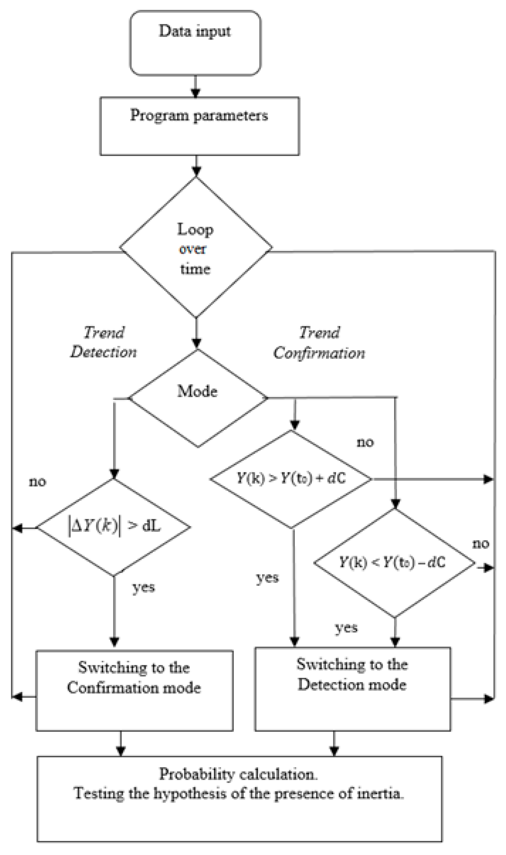
Figure 2.
An example of the dynamics of the EURUSD quotation over a 10-day observation period.

Figure 3.
Positive outcome examples.

Figure 4.
Negative outcome examples.

Figure 5.
An example of an analysis of a simple strategy based on the dynamics of linear trends over an interval of 10 days.
Figure 5.
An example of an analysis of a simple strategy based on the dynamics of linear trends over an interval of 10 days.

Figure 6.
Examples of incorrect trend detection due to a delay in decision making.

Figure 7.
Example of a decision-making scheme with two trends.

Figure 8.
Detection of an uptrend with first- and second-order approximations.

Figure 9.
Detection of a downtrend with first- and second-order approximations.

Figure 10.
Process, speed, and acceleration estimates.

Figure 11.
Inertia analysis results on a 5-day observation interval.


Table 1.
Positive outcome frequency at .
| Time Interval, Days | Currency Instruments | ||
|---|---|---|---|
| EURUSD | EURJPY | USDJPY | |
| 1–100 | 0.552 | 0.484 | 0.444 |
| 101–200 | 0.507 | 0.536 | 0.465 |
| 201–300 | 0.533 | 0.552 | 0.560 |
| 301–400 | 0.494 | 0.452 | 0.465 |
| 401–500 | 0.446 | 0.545 | 0.444 |
Table 2.
Positive outcome frequency at dL = 50.
| Time Interval, Days | Currency Instruments | ||
|---|---|---|---|
| EURUSD | EURJPY | USDJPY | |
| 1–100 | 0.539 | 0.568 | 0.522 |
| 101–200 | 0.524 | 0.528 | 0.497 |
| 201–300 | 0.529 | 0.503 | 0.537 |
| 301–400 | 0.503 | 0.550 | 0.534 |
| 401–500 | 0.493 | 0.548 | 0.552 |
Table 3.
The frequency of positive outcomes for positions that were opened using the smoothed process.
Table 3.
The frequency of positive outcomes for positions that were opened using the smoothed process.
| Time Interval, Days | EURUSD | ||
|---|---|---|---|
| 1–100 | 0.667 | 0.681 | 0.618 |
| 101–200 | 0.771 | 0.791 | 0.667 |
| 201–300 | 0.606 | 0.706 | 0.612 |
| 301–400 | 0.612 | 0.653 | 0.618 |
| 401–500 | 0.648 | 0.581 | 0.574 |
Table 4.
Positive outcome frequency for positions opened and closed by the smoothed process.
| Time Interval, Days | EURUSD | ||
|---|---|---|---|
| 1–100 | 0.652 | 0.652 | 0.593 |
| 101–200 | 0.698 | 0.706 | 0.696 |
| 201–300 | 0.686 | 0.707 | 0.688 |
| 301–400 | 0.612 | 0.612 | 0.582 |
| 401–500 | 0.567 | 0.534 | 0.574 |
Table 5.
Positive outcome frequency at .
| Time Interval, Days | EURUSD | EURJPY | ||||
|---|---|---|---|---|---|---|
| Scheme 1 | Scheme 2 | Scheme 3 | Scheme 4 | Scheme 5 | Scheme 6 | |
| 1–100 | 0.54 | 0.52 | 0.71 | 0.49 | 0.52 | 0.67 |
| 101–200 | 0.50 | 0.53 | 0.72 | 0.50 | 0.54 | 0.73 |
| 201–300 | 0.54 | 0.50 | 0.72 | 0.53 | 0.54 | 0.72 |
| 301–400 | 0.48 | 0.43 | 0.69 | 0.50 | 0.50 | 0.69 |
| 401–500 | 0.48 | 0.43 | 0.66 | 0.51 | 0.55 | 0.72 |
Table 6.
Positive outcome frequency for scheme 3.
| Time Interval, Days | EURUSD, dL = 75 | EURJPY, dL = 75 | ||||
| = 0.02 | 0.01 | 0.005 | 0.02 | 0.01 | 0.005 | |
| 1–100 | 0.69 | 0.61 | 0.71 | 0.57 | 0.62 | 0.68 |
| 101–200 | 0.72 | 0.76 | 0.75 | 0.72 | 0.74 | 0.81 |
| 201–300 | 0.66 | 0.66 | 0.65 | 0.70 | 0.73 | 0.78 |
| 301–400 | 0.55 | 0.57 | 0.60 | 0.67 | 0.70 | 0.79 |
| 401–500 | 0.58 | 0.59 | 0.63 | 0.68 | 0.71 | 0.79 |
| Time Interval, Days | EURUSD, dL = 50 | EURJPY, dL = 50 | ||||
| = 0.02 | 0.01 | 0.005 | 0.02 | 0.01 | 0.005 | |
| 1–100 | 0.58 | 0.63 | 0.70 | 0.63 | 0.70 | 0.71 |
| 101–200 | 0.70 | 0.72 | 0.80 | 0.75 | 0.76 | 0.82 |
| 201–300 | 0.71 | 0.76 | 0.78 | 0.72 | 0.76 | 0.80 |
| 301–400 | 0.66 | 0.67 | 0.72 | 0.70 | 0.71 | 0.75 |
| 401–500 | 0.65 | 0.67 | 0.68 | 0.70 | 0.73 | 0.77 |
Table 7.
Positive outcome frequency for scheme 3 and various trend confirmation levels.
| Time Interval, Days | EURUSD, dL = 100 | EURJPY, dL = 100 | ||||
|---|---|---|---|---|---|---|
| dC = 75 | dC = 50 | dC =25 | dC = 75 | dC = 50 | dC = 25 | |
| 1–100 | 0.63 | 0.67 | 0.74 | 0.64 | 0.79 | 0.75 |
| 101–200 | 0.75 | 0.75 | 0.90 | 0.75 | 0.79 | 0.84 |
| 201–300 | 0.72 | 0.73 | 0.79 | 0.66 | 0.65 | 0.84 |
| 301–400 | 0.62 | 0.63 | 0.76 | 0.55 | 0.68 | 0.81 |
| 401–500 | 0.60 | 0.61 | 0.72 | 0.59 | 0.63 | 0.83 |
Table 8.
Positive outcome frequency for scheme 3 and various trend detection levels.
| Time Interval, Days | EURUSD, dL = 75 | EURUSD, dL = 50 | ||||
|---|---|---|---|---|---|---|
| dC = 75 | dC = 50 | dC = 25 | dC = 75 | dC = 50 | dC = 25 | |
| 0–100 | 0.57 | 0.70 | 0.74 | 0.67 | 0.68 | 0.71 |
| 101–200 | 0.72 | 0.73 | 0.84 | 0.75 | 0.75 | 0.84 |
| 201–300 | 0.70 | 0.74 | 0.78 | 0.69 | 0.72 | 0.80 |
| 301–400 | 0.67 | 0.69 | 0.80 | 0.68 | 0.70 | 0.80 |
| 401–500 | 0.68 | 0.71 | 0.79 | 0.66 | 0.70 | 0.78 |
Table 9.
Frequency of trend confirmation for various parameter values.
| 0.025 | 0.05 | 0.075 | 0.1 | ||
|---|---|---|---|---|---|
| 0.025 | 25 | 0.50 | 0.48 | 0.49 | 0.49 |
| 0.025 | 50 | 0.51 | 0.50 | 0.51 | 0.50 |
| 0.025 | 75 | 0.50 | 0.50 | 0.50 | 0.51 |
| 0.025 | 100 | 0.50 | 0.51 | 0.51 | 0.51 |
| 0.05 | 25 | 0.50 | 0.48 | 0.48 | 0.50 |
| 0.05 | 50 | 0.50 | 0.50 | 0.51 | 0.50 |
| 0.05 | 75 | 0.50 | 0.50 | 0.51 | 0.50 |
| 0.05 | 100 | 0.50 | 0.51 | 0.51 | 0.51 |
| 0.075 | 25 | 0.50 | 0.49 | 0.49 | 0.49 |
| 0.075 | 50 | 0.50 | 0.50 | 0.50 | 0.50 |
| 0.075 | 75 | 0.50 | 0.50 | 0.51 | 0.51 |
| 0.075 | 100 | 0.51 | 0.51 | 0.51 | 0.51 |
| 0.1 | 25 | 0.50 | 0.48 | 0.48 | 0.49 |
| 0.1 | 50 | 0.50 | 0.51 | 0.51 | 0.50 |
| 0.1 | 75 | 0.50 | 0.50 | 0.50 | 0.50 |
| 0.1 | 100 | 0.50 | 0.50 | 0.50 | 0.51 |
Table 10.
Frequency of trend confirmation for various time intervals.
| Frequency of Trend Confirmation | ||||
|---|---|---|---|---|
| Days 1–100 | Days 101–200 | Days 201–300 | Days 301–400 | |
| 25 | 0.48 | 0.49 | 0.48 | 0.47 |
| 50 | 0.53 | 0.46 | 0.48 | 0.48 |
| 75 | 0.53 | 0.50 | 0.49 | 0.45 |
| 100 | 0.55 | 0.50 | 0.52 | 0.47 |
Table 11.
Frequency of trend confirmation for various widths of the sliding window.
| Frequency of Trend Confirmation | ||||
|---|---|---|---|---|
| w, min | Days 1–100 | Days 101–200 | Days 201–300 | Days 301–400 |
| 100 | 0.54 | 0.46 | 0.54 | 0.54 |
| 200 | 0.48 | 0.51 | 0.50 | 0.50 |
| 300 | 0.49 | 0.48 | 0.52 | 0.52 |
Table 12.
Parameter groups that determine trend detection and confirmation levels.
| Groups | 1 | 2 | 3 | 4 | 5 | 6 | 7 |
|---|---|---|---|---|---|---|---|
| dC | 75 | 100 | 50 | 75 | 75 | 75 | 75 |
| dL | 75 | 75 | 75 | 100 | 50 | 75 | 75 |
| dT | 1000 | 1000 | 1000 | 1000 | 1000 | 1000 | 1500 |
Table 13.
Frequency of inertia confirmation for various time intervals of observation for the initial data.
Table 13.
Frequency of inertia confirmation for various time intervals of observation for the initial data.
| Observation Interval Parameter Group | 1–100 | 101–200 | 201–300 | 301–400 | 401–500 |
|---|---|---|---|---|---|
| 1 | 0.51 | 0.54 | 0.46 | 0.47 | 0.52 |
| 2 | 0.36 | 0.54 | 0.54 | 0.47 | 0.50 |
| 3 | 0.49 | 0.45 | 0.43 | 0.49 | 0.49 |
| 4 | 0.57 | 0.59 | 0.46 | 0.55 | 0.50 |
| 5 | 0.58 | 0.51 | 0.46 | 0.42 | 0.53 |
| 6 | 0.61 | 0.81 | 0.84 | 0.41 | 0.43 |
| 7 | 0.56 | 0.55 | 0.47 | 0.45 | 0.48 |
Table 14.
Frequency of inertia confirmation for a smoothed stochastic process and various observation intervals using the smoothed component only to detect the trend.
Table 14.
Frequency of inertia confirmation for a smoothed stochastic process and various observation intervals using the smoothed component only to detect the trend.
| Observation Interval Parameter Group | 1–100 | 101–200 | 201–300 | 301–400 | 401–500 |
|---|---|---|---|---|---|
| 1 | 0.49 | 0.50 | 0.52 | 0.46 | 0.31 |
| 2 | 0.46 | 0.46 | 0.48 | 0.45 | 0.57 |
| 3 | 0.45 | 0.46 | 0.55 | 0.50 | 0.47 |
| 4 | 0.41 | 0.52 | 0.51 | 0.48 | 0.50 |
| 5 | 0.49 | 0.48 | 0.45 | 0.47 | 0.35 |
| 6 | 0.49 | 0.46 | 0.51 | 0.44 | 0.40 |
| 7 | 0.75 | 0.49 | 0.48 | 0.69 | 0.44 |
Table 15.
Frequency of inertia confirmation for a smoothed stochastic process and various observation intervals using the smoothed component to detect and confirm the trend.
Table 15.
Frequency of inertia confirmation for a smoothed stochastic process and various observation intervals using the smoothed component to detect and confirm the trend.
| Observation Interval Parameter Group | 1–100 | 101–200 | 201–300 | 301–400 | 401–500 |
|---|---|---|---|---|---|
| 1 | 0.55 | 0.82 | 0.85 | 0.46 | 0.44 |
| 2 | 0.22 | 0.68 | 0.88 | 0.27 | 0.43 |
| 3 | 0.69 | 0.81 | 0.83 | 0.54 | 0.39 |
| 4 | 0.47 | 0.72 | 0.77 | 0.24 | 0.31 |
| 5 | 0.55 | 0.76 | 0.87 | 0.54 | 0.33 |
| 6 | 0.61 | 0.81 | 0.84 | 0.45 | 0.44 |
| 7 | 0.56 | 0.86 | 0.90 | 0.45 | 0.71 |
Disclaimer/Publisher’s Note: The statements, opinions and data contained in all publications are solely those of the individual author(s) and contributor(s) and not of MDPI and/or the editor(s). MDPI and/or the editor(s) disclaim responsibility for any injury to people or property resulting from any ideas, methods, instructions or products referred to in the content. |
© 2023 by the authors. Licensee MDPI, Basel, Switzerland. This article is an open access article distributed under the terms and conditions of the Creative Commons Attribution (CC BY) license (https://creativecommons.org/licenses/by/4.0/).
Share and Cite
MDPI and ACS Style
Musaev, A.; Makshanov, A.; Grigoriev, D. Exploring the Quotation Inertia in International Currency Markets. Computation 2023, 11, 209. https://doi.org/10.3390/computation11110209
AMA Style
Musaev A, Makshanov A, Grigoriev D. Exploring the Quotation Inertia in International Currency Markets. Computation. 2023; 11(11):209. https://doi.org/10.3390/computation11110209
Chicago/Turabian StyleMusaev, Alexander, Andrey Makshanov, and Dmitry Grigoriev. 2023. "Exploring the Quotation Inertia in International Currency Markets" Computation 11, no. 11: 209. https://doi.org/10.3390/computation11110209
Note that from the first issue of 2016, this journal uses article numbers instead of page numbers. See further details here.