Review

Theoretical Understanding of Convolutional Neural Network: Concepts, Architectures, Applications, Future Directions

by
Mohammad Mustafa Taye
Data Science and Artificial Intelligence, Philadelphia University, Amman 19392, Jordan
Computation 2023, 11(3), 52; https://doi.org/10.3390/computation11030052
Submission received: 3 February 2023 / Revised: 2 March 2023 / Accepted: 3 March 2023 / Published: 6 March 2023

Abstract

:
Convolutional neural networks (CNNs) are one of the main types of neural networks used for image recognition and classification. CNNs have several uses, some of which are object recognition, image processing, computer vision, and face recognition. Input for convolutional neural networks is provided through images. Convolutional neural networks are used to automatically learn a hierarchy of features that can then be utilized for classification, as opposed to manually creating features. In achieving this, a hierarchy of feature maps is constructed by iteratively convolving the input image with learned filters. Because of the hierarchical method, higher layers can learn more intricate features that are also distortion and translation invariant. The main goals of this study are to help academics understand where there are research gaps and to talk in-depth about CNN’s building blocks, their roles, and other vital issues.

1. Introduction

There has been a dramatic surge in the usage of machine learning (ML) in recent years [1,2,3] for a wide range of purposes, from research to practical applications, including text mining, spam detection, video recommendation, picture categorization, and multimedia idea retrieval [4,5].
Deep learning (DL) is one machine learning (ML) approach that is commonly used in these contexts [6,7]. The working domain of DL is a subset of that of ML and artificial intelligence (AI); therefore, it may be seen as a function of AI that mimics the way the human brain processes information [1]. The traditional neural network from which DL originated has significantly been surpassed by its superior performance. In addition, DL uses transformations and graph technologies in tandem to construct multi-layer learning models [8,9].
A closer examination of the “Learning sub-fields” reveals that deep learning (DL), a subfield of machine learning (ML), focuses on creating algorithms that simulate how the human brain thinks and solves problems [5,8,10].
Recent years have seen a surge in interest in machine learning algorithms, which are now being used in various fields, including image recognition, optical character recognition, pricing prediction, spam filtering, fraud detection, healthcare, transportation, and many others [11]. The various machine-learning types and algorithms are depicted in Figure 1.
Over the past few years, deep learning has recently received a lot of attention and has been applied successfully in addressing a wide range of problems in various application fields. Diverse deep-learning techniques are applied in several application areas [4].
These application areas include robots, enterprises, cybersecurity, virtual assistants, image recognition, and healthcare. They also involve sentiment analysis and natural language processing [8].
The most established deep learning technique is the convolutional neural network (CNN), a subtype of an artificial neural network [12]. Since the astounding outcomes of the ImageNet Large Scale Visual Recognition Competition, an object recognition competition, in 2012 [13,14], CNN has dominated computer vision tasks.
CNN is useful in medical imaging because it can detect tumors and other irregularities more accurately in X-ray and MRI images. CNN models can analyze a picture of a human body component, such as the lungs, and identify potential tumor locations as well as other abnormalities like fractured bones in X-ray images based on previously processed comparable images by CNN networks [15,16,17].
Convolutional neural networks (CNN), which are used to represent spatial information, may be used to model images.
Because of their greater capacity to extract features from pictures, such as barriers and road signs, CNNs are characterized as universal non-linear function approximators.
CNN has been used for biometric user identity authentication by recognizing particular physical characteristics associated with a person’s face. CNN models may be trained on photos or videos of individuals to recognize certain features of their faces, such as the distance between their eyes, the shape of their noses, and the curve of their lips [15,16,17].
Most of the time, convolutional neural networks have led to ground-breaking discoveries in many fields related to pattern recognition, such as voice and image processing.
The number of ANN parameters going down is the most important thing about CNNs [18,19].
This success has encouraged researchers and developers to utilize more complex models to tackle difficult issues that conventional ANNs were unable to address. The most important presupposition regarding the issues that CNN resolves is that there should be no spatially dependent characteristics [19].
CNN is to blame for the current popularity of DL. The primary benefit of CNN over its forerunners is that it does everything automatically and without human supervision, making it the most popular. Therefore, we have covered a lot of ground with CNN by outlining its essential parts. The most prevalent CNN architectures, starting with the AlexNet network and concluding with the high-resolution network, have also been explored in length (HR.Net) [19,20].
This review’s main objective is to draw attention to the elements of CNN that are most important, making it simple for researchers and students to comprehend CNN completely after reading just one review paper. Additionally, in order to encourage CNN research, we want to let people understand more about current developments in the industry. In view to provide more precise options to the field, researchers would be allowed to select the best route of study to follow.
CNNs learn as they are trained on images; therefore, the features they extract from images are not pre-learned.
Automatic feature extraction is largely responsible for the remarkable success of deep learning models in computer vision. Complex models are required for deep CNN architecture. More precision from them calls for larger image databases. For computer vision tasks like object categorization, detection, tracking, and recognition, CNNs need access to huge labeled datasets.
Object identification, which has captivated researchers for much of this decade, has significantly benefited from the application of deep learning techniques. Object identification and tracking play a crucial role in video surveillance, making it one of the most difficult but vital aspects of security systems. It keeps an eye on people in public places to spot any signs of unusual or suspicious conduct.
The general contribution of this study is summarized as follows:
This review almost provides an in-depth analysis of CNN’s most important features.
This review almost provides an in-depth analysis of CNN’s networks and algorithms.
In this paper, I have compiled all of the current deep learning-based object detection methods that can be found in the most recent academic literature.
To help pick the best object detection method for a given application or dataset, I reviewed and compared several popular options.
This article focuses on CNN’s models and processes.
We put together a list of CNN to help developers and academics learn more about how to use CNN.
We explain CNN in-depth, the most well-known deep learning algorithm, by outlining the ideas, theories, and cutting-edge architectures.

Survey Methodology

I have analyzed the key research articles published in the field between 2017 and 2022, with a focus on those from 2017, 2018, and 2019, along with a few from 2021 and 2022. The primary emphasis was on publications from the most prestigious publishers, including IEEE, Elsevier, MDPI, ACM, and Springer. Several papers from ArXiv have been chosen. I have examined over 60 papers on a variety of DL-related topics. There are 14 papers from 2017, 12 papers from 2018, 19 papers from 2019, and 15 papers from all other years (2020–2022). This shows that the focus of this review was on the most recent publications in DL and CNN. The selected publications were analyzed and evaluated in order to perform the following:
(1)
List and describe the DL and CNN techniques and network types;
(2)
Present the problems of CNN and provide alternative solutions;
(3)
List and explain CNN architectures;
(4)
Evaluate the applications of CNN.
“Deep Learning”, “Machine Learning”, “Convolution Neural Network”, “Convolution Neural Network” and “Architectures”, “Convolution Neural Network” and “detection” or “classification” or “segmentation” and “Convolution Neural Network” and “Overfitting” are the most common search terms for this review.

2. Convolutional Neural Network (CNN or ConvNet)

Convolutional neural networks (CNNs) are artificial intelligence systems based on multi-layer neural networks that can identify, recognize, and classify objects as well as detect and segment objects in images. In fact, CNN or ConvNet is a popular discriminative deep learning architecture that could be learned directly from the input object without the obligation for human feature extraction [15,16,17].
This network is frequently used in visual identification, medical image analysis, image segmentation, NLP, and many other applications since it is specifically designed to deal with a range of 2D shapes [15,16,17]. It is more effective than a regular network since it can automatically identify key elements from the input without the need for human participation.

2.1. CNN Fundamentals

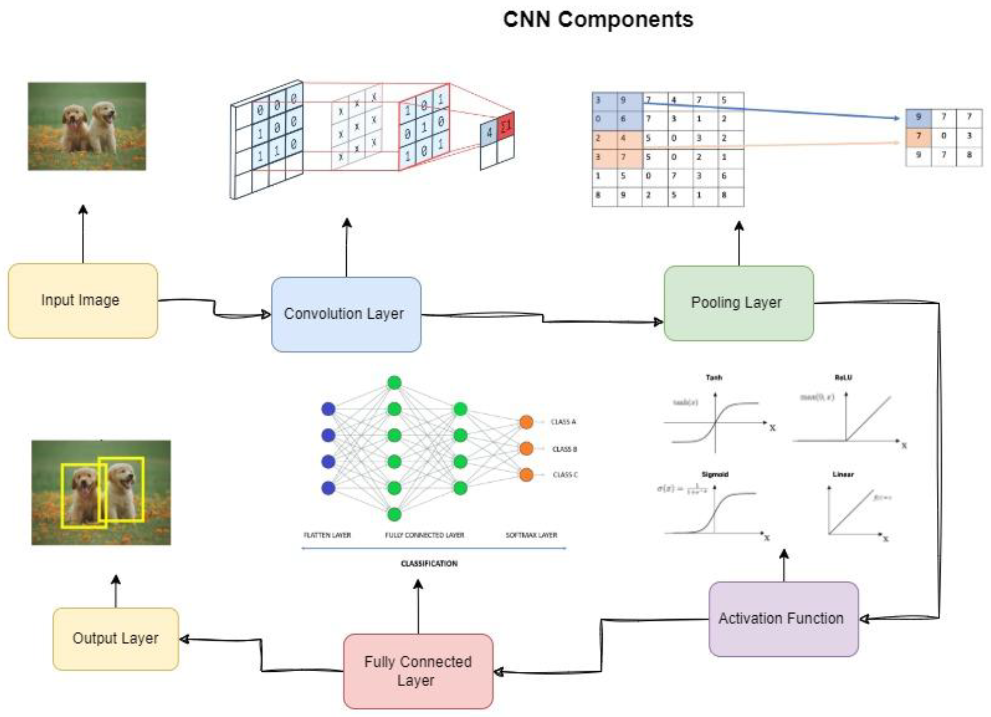
Understanding the various CNN components and their applications is critical to comprehending the advancements in CNN architecture. Figure 2 displays several CNN parts.
CNN Layers
A CNN is typically composed of four types of layers
  • Convolutional;
  • Pooling;
  • Function of Activation;
  • Fully Connected.

2.1.1. Input Image

The building blocks of a computer image are called pixels. They are the binary of the visual data representation. From 0–255 pixels are sequentially organized in a matrix-like arrangement in the digital image’s layout. The brightness and hue of each pixel are specified by its pixel value [15,16,17].
When viewing an image first, humans’ brains assimilate a tremendous amount of information.
The CNN layers are trained to first recognize more basic patterns, such as lines and curves, before moving on to more intricate patterns, such as faces and objects. As a result, it is possible to assert that using a CNN could provide computers with vision [15,16,17].

2.1.2. Convolutional Layer

The convolutional layer is a crucial part of CNN’s overall structure. It is a set of filters—or kernels—applied to the data before it is used. Each kernel’s width, height, and weight are used to extract characteristics from the input data. Weights in the kernel are first assigned at random but gradually become more informed by the training data.
In other words, the feature map is made by combining the input image (which is shown by N-dimensional metrics) with these filters [15,16,17].
A kernel is a set of discrete values or integers.
For each number, the kernel weight is given as a reference. The initial kernel weights for a CNN are a set of integers picked at random. Additionally, the weights are initialized in various ways. In turn, the kernel learns to extract meaningful features because these weights are tweaked during the training process.
The kernel enables them to perform the operation in a high-dimensional, implicit feature space without calculating the coordinates of the data in that space. Instead, they compute the inner product of the pictures of all data pairings in feature space. By applying the kernel trick to a linear model, it can be transformed into a non-linear model.
The CNN input format is first provided before the convolutional process begins. The classic neural network takes in data in a vector format, whereas the CNN takes in a multi-channeled image. While an RGB image contains three color “channels,” a grayscale image has just one.
Examine this 4 × 4 grayscale image with a 2 × 2 random weight-initialized kernel to learn about convolutions in action. The kernel will first pan horizontally and vertically over the full picture. The dot product between the input picture and the kernel is also computed in parallel; this is accomplished by multiplying the corresponding values and adding the results to get a single scalar value. Thereafter, the procedure is repeated until no more sliding is feasible [15,16,17].
The main image (K), the filter (L).
The output matrix is based on the equation
(K − L + 1),
4 − 2 + 1 = 3, so the output then 3 × 3
In fact, the values of the dot product indicate the feature map of the output. Figure 3 visually represents the primary calculations performed at each stage. In this diagram, the smaller square (2 × 2) represents the kernel, while the larger square (4 × 4) represents the input picture. A product is then presented as a number after multiplying by both, and this sum provides an input value for the output feature map [15,16,17].
However, in the preceding example, the kernel is given a stride of 1 (designating the desired step size total for vertical or horizontal locations), but the input image is not padded. Indeed, you are free to substitute a different stride value if you so choose. An additional benefit of increasing the stride value is a decrease in the dimensionality of the resulting feature map [15,16,17].
The border size of the supplied picture, however, is greatly influenced by padding.
In contrast, the characteristics of the border side change dramatically over time.
Padding makes the input picture bigger, which also makes the size of the feature map bigger.
Each filter could represent a feature. The filter does not activate when it moves over an image and does not discover a match. CNN employs this method to discover the most effective object–description filters.
Figure 4 demonstrates how the matrix may be configured to find picture edges. Due to the fact that they behave like the conventional filters used in image processing methods, these matrices are also known as filters.
In CNN, however, these filters are started before the form filters used in the training process, which are better suited to the job at hand.
Weight Sharing: Since the entire set of weights in a CNN act on each and every pixel of the input matrix, there are no assigned weights between any two neurons in nearby layers. Learning a single group of weights for the entire input will significantly reduce the necessary training time and various costs because additional weights for each neuron do not need to be learned.
Stride: In fact, CNN offers additional options that provide several opportunities to further narrow the settings while also reducing some of the undesirable impacts. One of these options is called stride. In the aforementioned scenario, the next-layer node is assumed to have numerous overlaps with its neighbors based only on an examination of the areas. We may modify the overlap by changing the stride. A unique 6 × 6 image is shown in Figure 5. Since the filter can only be moved in one-node increments, the maximum output size we can achieve is 4 × 4. As can be seen in Figure 5, there is an overlap between the output of the three left matrices (and the three middle ones together and the three right ones also). However, if we walk, counting each step as 2, the total will be 3 times 3. In other words, the total output size and total overlap will be reduced [5,12,16].
Equation (2) formalizes this, resulting in the output size O as shown in Figure 6, given the image’s NXN dimension and FXF filter size.
  O = 1 + ( N F ) / S  
where N is the input size, F is the filter size, and S is the stride size.
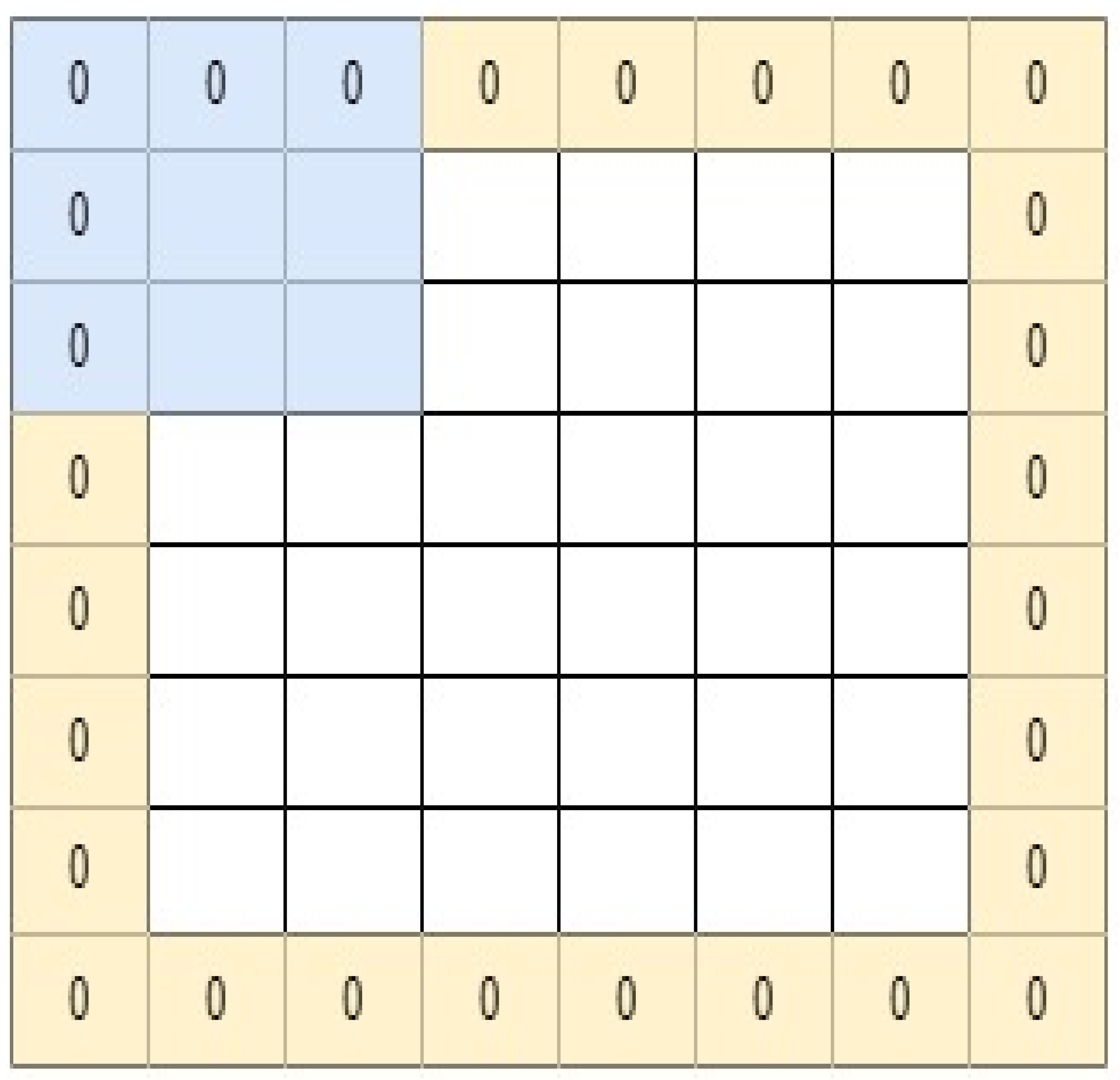
Padding: One disadvantage of the convolution step is the possible loss of detail at the image’s edges. They are only captured when the filter is moved, so they are never actually seen. One easy and practical solution is to use zero padding. You may also manage the output size with the aid of zero padding.
In Figure 6, for instance, the output will be 4 × 4 (which decreases from a 6 × 6 input) with N = 6, F = 3, and stride 1.
However, by including one zero-padding, the result will be 6 × 6, which is identical to the initial input (the calculation for actual N now being 9). The formula is a modified formula with zero padding (3).
O = 1 + N + 2 P F S
where P is the number of the layers of the zero-padding (e.g., P = 1 in Figure 7), We can avoid network output size from decreasing with depth by using this padding concept. Consequently, any number of deep convolutional networks is feasible [21].
Feature of CNNs: Due to the aforementioned weight distribution, the model is also invariant under translational changes. The learn function may be filtered to help in any environment. If beginning with random values for the filters improves performance, then the filters will learn to detect the edge (as in Figure 3). It is crucial to note that a shared weight is a bad idea when evaluating an input’s spatial significance.

2.1.3. Pooling

The pooling layer, also known as the down-sampling layer, is used to decrease the feature maps’ dimensionality while retaining the most important data. A filter applies the pooling operation to the input data by sliding over it in the pooling layer (max, min, avg). In the literature, maximum pooling is most frequently utilized.
The essential part of pooling, which is utilized to reduce the complexity of upper layers, is down-sampling. In terms of image processing, it may be comparable to reducing the resolution. Filter count is unaffected by pooling. Max-pooling is one of the most often used pooling methods. The picture is divided into rectangular subregions, and only the greatest value discovered inside each subregion is returned. One of the most prevalent max-pooling sizes is 2 × 2.
As shown in Figure 8, when pooling is used on the 2-by-2 blocks in the top-left corner, attention is diverted to the top-right corner, and two steps are moved. As a result, stride 2 is used for pooling. It is possible to use stride 1, which is unusual, to prevent downsampling. Keep in mind that downsampling does not preserve the position of the data.
At various pooling levels, various pooling techniques may be applied. Global average pooling (GAP), global max pooling, average pooling, min pooling, and gated pooling are some of these methods. Figure 8 depicts each of these three pooling techniques [22,23].
The primary problem with the pooling layer is that it does not aid CNN in determining whether or not a feature is present in an input image but rather just where that feature is located. Therefore, there are times when CNN’s total ratings take a dip. However, the CNN model leaves out the necessary information.

2.1.4. Non-Linearity (Function of Activation)

The layer of non-linearity follows convolution. Non-linearity allows the generated output to be changed or terminated. This layer is used to restrict or oversaturate the output.
Every type of activation function in every type of neural network serves the essential function of mapping input to output. The input value is calculated by calculating the weighted sum of the neuron input and its bias (if present). This indicates that the activation function determines whether or not to fire a neuron in response to a certain input by generating the matching output.
In the CNN architecture, non-linear activation layers are used after all layers with weights (also known as learnable layers, such as FC layers and convolutional layers).
The mapping of input to output will be non-linear because of the activation layers’ non-linear performance, and these layers also enable the CNN to learn extremely complex things [22,23,24].
Additionally, the capacity to differentiate is a crucial requirement for the activation function since it enables the use of error backpropagation to train the network.
The most popular activation functions in CNNs and other deep neural networks are the ones listed below:
Sigmoid: This activation function only allows output values between 0 and 1 and accepts real numbers as input [25,26,27,28].
Tanh: It is comparable to the sigmoid function in that it accepts real numbers as input, but its output range is only between one and one.
ReLU is the most popular function in the CNN context. All of the input values are converted to the positive range. ReLU’s primary benefit over other algorithms is the time and resources it saves when used.
For a long time, the Tanh and sigmoid non-linearities were the most prevalent. Non-linearities come in many forms, and they are shown in Figure 9. For these reasons, however, the rectified linear unit (ReLU) has seen a surge in popularity in recent years.
Function and gradient definitions using ReLU are simpler.
Saturated functions, such as the sigmoid and the tanh, have issues with backpropagation. This phenomenon, known as the “vanishing gradient,” occurs when the gradient signal gradually decreases as the depth of the neural network architecture grows. This happens because the gradient of these functions is essentially zero on all sides of the center. Nonetheless, the ReLU has a constant gradient for the positive input. While the function cannot be distinguished, it can be ignored during implementation.
Third, the ReLU generates a sparser representation because a complete zero is produced by a gradient zero. For sigmoid and tanh, the gradient outcomes are never zero, which may be counterproductive during training [22,23,26,27,28,29].
When using ReLU, a few significant problems may occasionally arise.
Consider a method for error backpropagation with a greater gradient flowing through it, for instance.
The weights will be updated by passing this gradient through the ReLU function in a way that ensures that the neuron will not be stimulated again.
This problem is known as “Dying ReLU”.
In order to address these problems, there are some ReLU substitutes.
These are some of them, as discussed below.
Leaky ReLU: This activation function makes sure that the negative inputs are never disregarded, as opposed to the negative inputs being downscaled by ReLU. It is used to address the Dying ReLU issue.

2.1.5. Fully Connected Layer

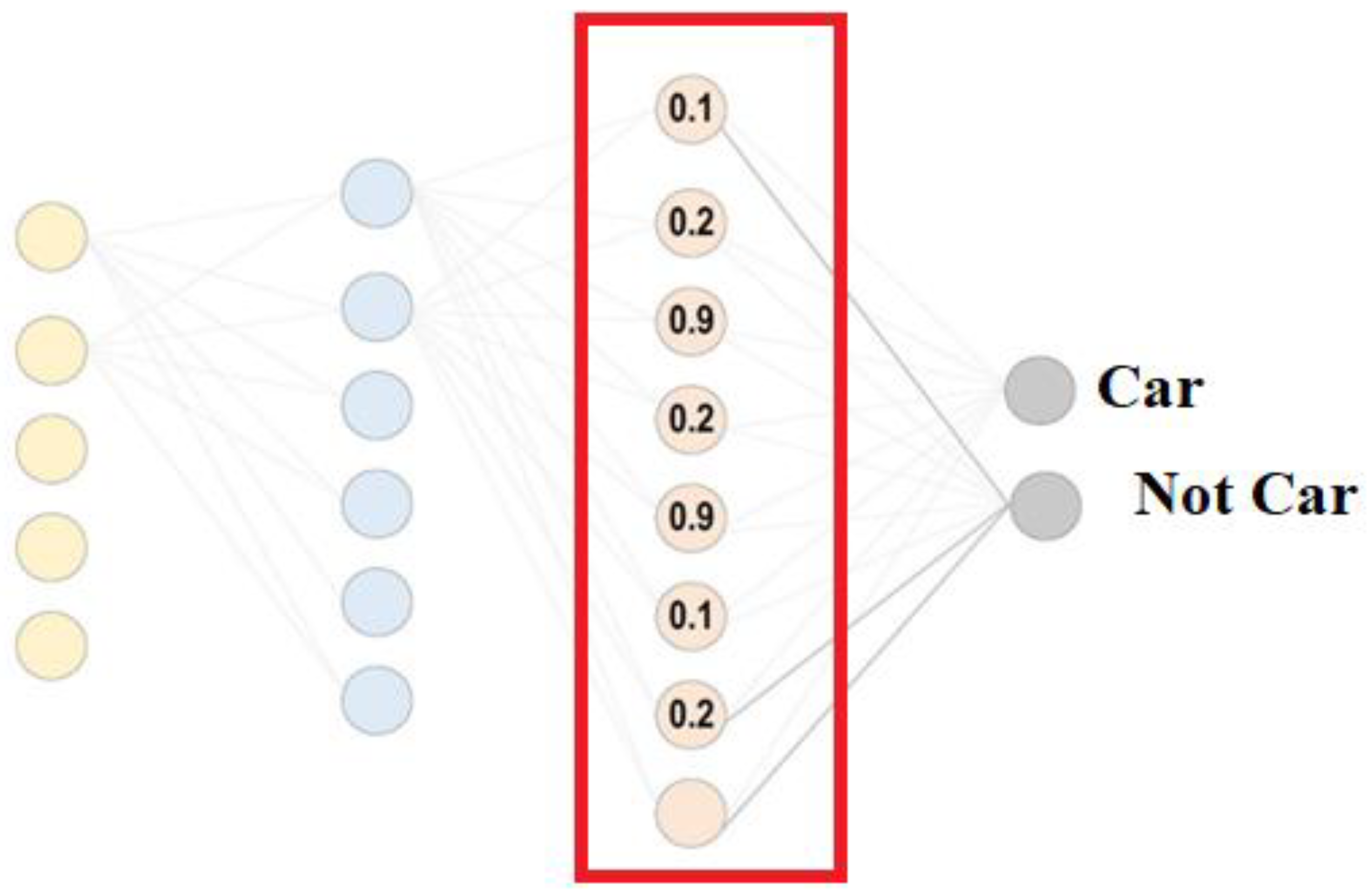
Neurons are organized into groups in the fully-connected layer that are reminiscent of those seen in traditional neural networks. As shown in Figure 10, any node in a layer that is entirely linked is, therefore, directly connected to every node in the layer above and below it. Figure 10 shows that every node in the pooling layer’s most recent frames is connected as a vector from the fully-connected layer to the top layer. These are the most often utilized CNN parameters within these layers; however, they need a lot of training time [22,23,24].
The biggest drawback of a fully connected layer is the large number of parameters that necessitate laborious calculation in training samples. Consequently, we try to minimize the number of connections and nodes. The eliminated nodes and connections can be satisfied using the dropout approach. LeNet and AlexNet, for example, developed a vast and deep network while preserving a constant computational complexity [22,23].
The convolution, which is the core element of the CNN network, is exposed when the non-linearity and pooling layer is added. The three that are most commonly utilized in architecture are as follows:
To rephrase, in a completely connected layer, all of the neurons communicate with their counterparts in the layer below. It is a classifier used by CNN.
Being a feed-forward ANN, it performs similarly to a regular multi-layer perceptron network. Input to the FC layer comes from the last pooling or convolutional layer.
This is a vector input created by increasing the thickness of the feature maps [24].
Figure 10 displays that the FC layer’s output is consistent with the final CNN output.
The preceding part discussed the various types of layers used in the CNN design; this section will focus on loss functions.
Furthermore, the final classification is achieved by employing the output layer, the very last layer of the CNN architecture. A few loss functions are used in the CNN model’s output layer to compute the predicted error across the training data. As a result of this mistake, the disparity between actual and predicted output is highlighted. Then, it will be improved using the CNN learning approach.
The loss function, however, takes advantage of two inputs to pinpoint the source of the mistake. For CNN, the first parameter is the forecast or estimated output. The second input is the desired output or label. There are many different kinds of loss functions used for different sorts of problems [25].
Below is a basic explanation of the many kinds of loss functions:
Training: A training dataset made up of a collection of images and labels (classes, bounding boxes, and masks) is used to train a CNN model.
Backpropagation is a CNN training procedure that measures an error value using the output value of the previous layer. Each neuron’s weight in that layer is updated using the error value [26].
In order to measure an incorrect value and revise the old weights, fresh weights are employed, as shown in Figure 11.
Until it reaches the first layer, the algorithm repeats the procedure.
All inputs, including the bias unit, are summarized by the activation unit; then, use the activation function to compute the result. The network will then calculate the cost function and send the error back to update the weights until the cost is minimized.

3. Regularization of CNN

When trying to create well-behaved generalizations for CNN models, over-fitting is the key obstacle. Over-fitting describes a situation in which a model does well on training data but poorly on test data (data it has never seen before), as will be shown in the next section. When the model does not pick up enough information from the training data, it is said to be under-fitted [26,27,28].
A model is considered to be “just fit” if it produces satisfactory results on both the training and testing data. These three types are shown in Figure 12.
Multiple intuitive conceptions are used to facilitate regularization and prevent over-fitting; more details on over-fitting and under-fitting are provided below.
Using a dropout as a generalization strategy is popular. Neurons are removed at random throughout each training session. As an added bonus to coercively training the model to acquire several features, this method also makes feature selection equally weighted across the whole neural network.
A dropped neuron will not take part in either backward or forward propagation during training. Testing makes use of the full-scale network to make predictions [29,30].
The drop-weight method is quite similar to the dropout strategy. Drop-weight training differs from dropout in that only the weights (connections) between neurons are eliminated after each training iteration.
Data augmentation may easily prevent over-fitting when the model is trained using an enormous amount of data. In order to do this, data augmentation is needed. There are a few methods that may be utilized to increase the size of the training dataset artificially. Finally, data augmentation methods are discussed in further depth.
Through batch normalization, the efficacy of the final activations may be ensured [31,32].
The one-unit Gaussian distribution describes this execution well. When normalizing the output at each layer, we will first remove the mean and then divide it by the standard deviation.
Despite being conceptualized as a pre-processing activity at each tier of the network, this may be differentiated and integrated with other networks.
It is also employed to reduce “internal covariance shift” in the activation layers. The activation distribution’s variability defines the change in internal covariance at each layer.
The continual update of weights during training, which might occur if training data samples come from a wide range of sources, amplifies this change (for example, day and night images). However, the training period will lengthen since the model needs more time for convergence. For this reason, we add a layer to the CNN design that mimics batch normalization to help us deal with this issue [33,34,35].
The following are some benefits of using batch normalization:
  • It stops the disappearing gradient issue before it starts.
  • It has the ability to effectively manage bad weight initialization.
  • It significantly reduces the amount of time needed for network convergence (which will be very helpful for large datasets).
  • It has difficulty reducing training dependence on various hyperparameters.
  • Over-fitting is less likely because it only slightly affects regularization [35].

4. Popular CNN Architecture

R-CNN [36,37,38] was the first ground-breaking model to use convolution neural networks (CNN). For each image that needs to be classified, the model creates 2000 region proposals and resizes them to 227 × 227. R-CNN employs a region-of-interest (RoI) classifier based on a deep convolutional neural network (DCN) to perform region-specific classification of input pictures. In addition, a convolutional neural network (CNN) is employed for feature extraction and model training, and then a support vector machine (SVM) classifier is used for object categorization. This model moves at a snail’s pace. Eventually, in 2015, Fast R-CNN was offered as a solution to the accuracy and speed issues [37,38]. RoI extraction from feature maps is the focus of SPPNet and Fast R-CNN, an enhanced form of R-CNN. It was discovered that this method outpaced the standard R-CNN framework by a significant margin.
Faster R-CNN continues the trend by proposing region proposal networks for feature extraction and to eliminate storage costs [37,38]. Faster R-CNN, an enhanced variant of Fast R-CNN achieved using RPN-based fully-contained end-to-end training (region proposal network). Regression-based region-of-interest (RoI) networks (RPNs) are a type of network used in the process of producing RoIs.
Compared to earlier models, this one performs well in terms of accuracy and speed; however, the ground truth and predicted bounding boxes are not aligned. To deal with the issue of inaccuracy generated by the quantization process in the region of interest (RoI) pooling layer, the authors introduce Mask R-CNN.
Mask R-CNN builds on top of the Faster R-CNN by including a mask prediction branch; this allows it to detect objects and predict their masks simultaneously. R-FCN swaps out the fully connected layers with position-aware score maps, which results in improved object detection.

Several CNN Architectures

CNN has many architectures, such as VGG, AlexNet, Xception, Inception, and ResNet [37,38,39,40,41,42,43,44,45,46,47,48,49], which can be used in different application domains depending on how well they can learn.
The convolutional neural network (CNN) is the most emblematic deep learning model. It comprises the input, convolution, pooling, and full connection layers [37,38,39,40,41,42,43,44,45,46,47,48,49]. The majority of existing networks are based on a series of CNN enhancements. LeCun first presented the LeNet network for handwritten digit identification in 1998 and extended CNN to the field of picture recognition. LeNet is an early neural network with only three complete connection layers, two convolution layers, and two pooling layers. Due to the tiny size of the model, it is unable to adequately fit other data, which hinders the advancement of computer vision areas.
In 2012, Krizhevsky proposed the AlexNet, resulting in a significant learning spike in computer vision. AlexNet has five convolutional layers and two fully linked layers for learning features are present in AlexNet. After the first, second, and fifth convolutional layers, it has max-pooling. It has 630M connections, 60M parameters, and 650K neurons altogether. The AlexNet was the first to demonstrate the use of deep learning for computer vision applications [44].
LeNet and AlexNet used a single convolutional layer with big kernels of size 7 × 7 and 11 × 11, while the VGG-16 was built with stacks of convolutional layers with smaller kernels of size 3 × 3.
By adding more non-linear rectification layers, a stack of convolutional layers with tiny filter sizes creates a more discriminatory decision function [39,44].
ZFNet [44] made modest modifications to the AlexNet network in 2013, mainly offering a new visualization technique. In the past, CNN was a black box; no theory or methodology was used to explain the network’s optimization and improvement process. Using deconvolution, ZFNet visualizes the intermediate layer of features [44]. Simonyan [40] introduced the VGG model in 2014, which investigates the effect of network depth on accuracy. Unlike AlexNet, VGG uses many convolution layers of size 3 × 3 to replace large-scale filters. The framework of the model is simple and effective, and it can be easily ported to other networks; nevertheless, the parameters are too large and simple to adjust. Researchers have effectively utilized VGG in numerous domains [31,32,33]. GoogLeNet [44] is a network that not only investigates the impact of depth but also considers the breadth of the network. The network eliminates the final full connection layer and intelligently implements the 1 × 1 convolution operation in order to lower the dimension and prevent the over-fitting issue caused by excessively large network parameters. The year 2015 saw the proposal of the ResNet residual network and residual connection by He et al. [44]. As a result, the depth of the network can reach 152 layers. The network employs a small number of pooling layers and a high number of downsampling, which increases the forward propagation efficiency of the network and obtains the greatest picture recognition effect at that time, demonstrating the viability of residual connection [46,47]. Liu et al. proposed DenseNet [39,44,45] in 2017. Using the ResNet network’s strategy for increasing the depth and width of the network can also guarantee the model’s precision. DenseNet created a network for typing. All information layers are concatenated (dimensionally coupled) with one another. DenseNet may efficiently minimize the number of parameters and increase the reusability of features across many convolutional layers [40,41,42,43,44]. Table 1. is shown a comparison between different popular CNNs Architecture. In 2018, boosting deep convolutional neural networks (BoostCNN). Use a deep learning architecture with a least-squares-based objective function and add boosting weights to learn this model. This model uses various network architectures within the proposed boosting framework, with BoostCNN choosing the most effective network architecture after each iteration.
The compound coefficient method was used by EfficientNet in 2019 to efficiently and effectively scale up models. Compound scaling uses a uniform set of scaling coefficients to increase an image’s width, depth, or resolution rather than randomly selecting one of these values. The authors of the paper efficiently used the scaling method and AutoML to create seven models of varying dimensions that both outperformed and were more efficient than the state-of-the-art convolutional neural networks.
CNNs have an advantage over other classification algorithms like SVM, K-NN, Random Forest, and others because they learn the most important features to represent the objects in an image.

5. Different Types of CNN Architectures

5.1. Classification

Image classification is crucial to the processing of multimedia information in the Internet of Things (IoT). In order to identify whether or not the illness is present, the image classification procedure uses the input images to provide an output classification. Image classification and recognition technology have found widespread usage in artificial intelligence applications, particularly in the areas of picture information retrieval, real-time target tracking, and medical image analysis. Recent years have seen a rise in interest in deep learning [50,51].
Popular CNN for classification tasks such as VGG-16, ResNets, and Inception [44].

5.2. Detection

The difficult computer vision task of object detection involves anticipating both the location of the objects in the image and the kind of objects that were found. Beginners may find it difficult to differentiate between various related computer vision tasks.
For instance, the distinctions between object localization and object detection might be difficult to understand, even though all three tasks may be collectively referred to as object recognition. Image categorization, by contrast, is straightforward.
Image classification involves assigning a category label to an image, whereas object localization involves drawing a bounding box around one or more objects in an image [52,53,54].
The more challenging object detection challenge involves doing both of these things at once, drawing bounding boxes around each object of interest in the image and then labeling each object with its class.
Together, we call these problems in the real world “object recognition”.
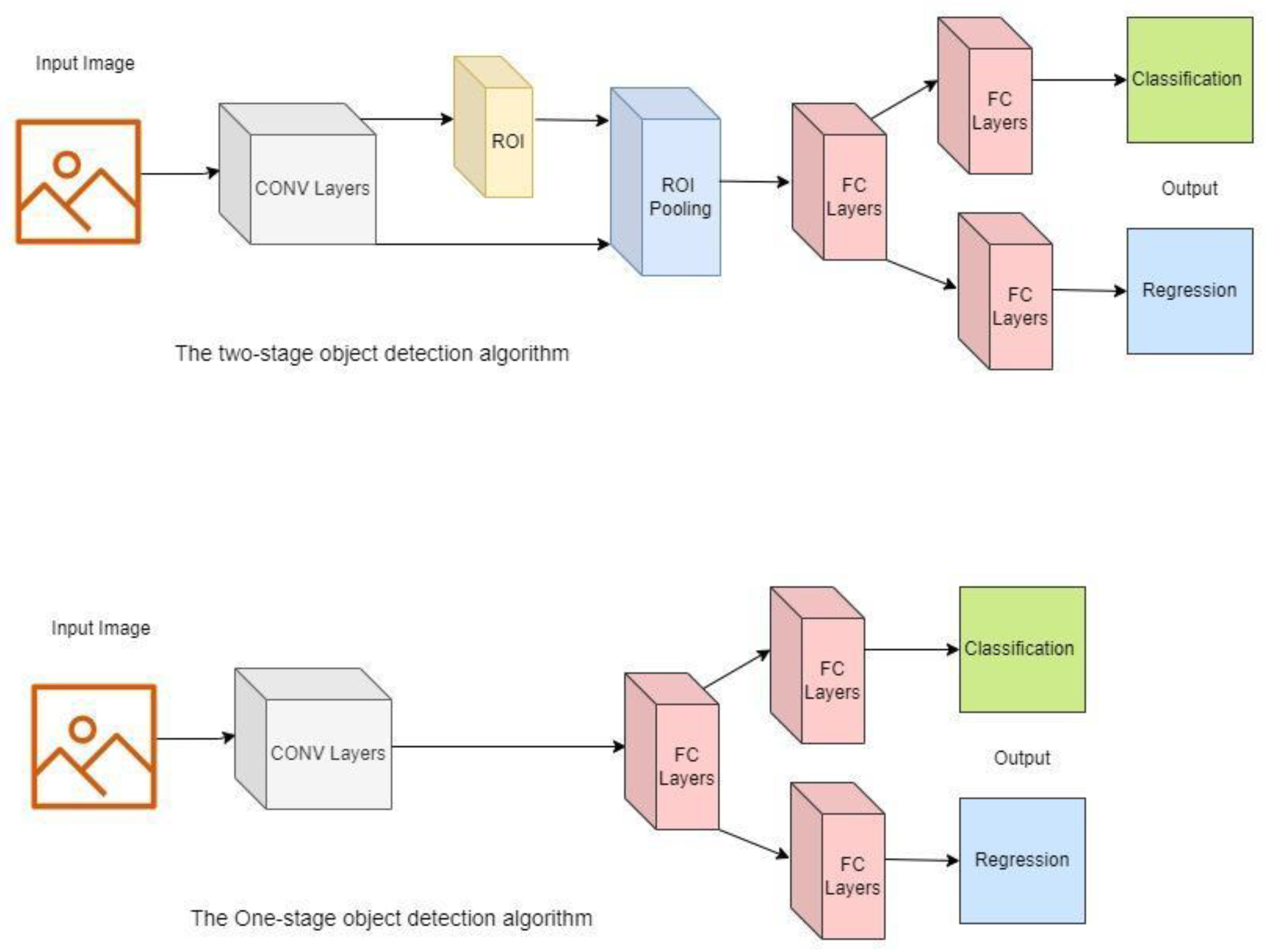
The process of object detection can be broken down into two distinct phases, as shown in Figure 13:
One-step object detectors.
The use of two-stage object detectors.
Object detectors that are built on two-stage deep learning pipelines have two distinct phases: (1) proposing regions and then (2) classifying the objects within those regions [37,38,43,44,55]. The object detector’s region proposal stage entails proposing a number of Regions of Interest (ROIs) in an input image that has a high possibility of having items of interest. The second phase involves selecting promising ROIs (while discarding less promising ones) and classifying items contained within them [53]. RCNN, Fast R-CNN, and Faster R-CNN are all well-liked examples of two-stage detectors. On the other hand, single-stage object detectors build bounding boxes and classify objects all in the same stage using a single feed-forward neural network. Although these detectors are quicker than their two-stage counterparts, they are often less precise. YOLO, SSD, EfficientNet, and RetinaNet are just a few of the most well-known examples of single-stage detectors. The distinction between these two object detectors is seen in Figure 13.
As one of the earliest deep learning-based object detectors, R-CNN implemented a two-stage detection process that included a highly effective selective search method for ROI proposals. A few issues with the R-CNN model were addressed with the introduction of fast RCNN, including slow inference speed and inaccurate predictions. The Fast R-CNN model uses a convolutional neural network (CNN) to process an image’s data and produce a feature map and ROI projection. Using ROI pooling, these regions of interest are mapped to the feature map for prediction. Rapid R-CNN is an alternative to R-CNN that bypasses the region of interest (ROI) as input to the CNN layers and instead processes the entire image to create feature maps for object detection [37,38]. While both Fast and Faster R-CNN use a similar strategy, Faster R-CNN uses a separate network to feed the ROI to the ROI pooling layer and the feature map, which are subsequently reshaped and used for prediction [37].
Due to their ability to make predictions about an input with just one pass, single-stage object detectors like YOLO (You only look once) are quicker than their two-stage counterparts. The first YOLO variation, YOLOv1, discovered how to quickly detect objects by learning generalizable representations of them [16]. While YOLOv1 used a fully connected layer to generate bounding boxes, YOLOv2 introduced batch normalization and a high-resolution classifier in 2016 [43,45]. YOLOv3 was proposed in 2018 [43,45] using a 53-layer backbone-based network that predicted overlapping bounding boxes and smaller objects using an independent logistic classifier and binary cross-entropy loss. In contrast to YOLO models, which produce feature maps by constructing grids within an image, SSD models were offered as a superior choice to execute inference on videos and real-time applications since they share features between the classification and localization task on the complete picture. Although YOLO models are quicker to run, they are not as accurate as SSD models [45]. While YOLO and SSD models offer fast inference speeds, they struggle with class imbalance when identifying tiny objects. The RetinaNet detector [20] overcame this problem by using a dedicated network for classification and bounding box regression during training and a focal loss function. Better methods for data augmentation and regularization during training (‘bag of freebies’) and a post-processing module that enables better mAP and faster inference (‘bag of specials’) were introduced in YOLOv4 [45]. YOLOv5 was proposed, which would further improve data augmentation and loss calculation. It also used self-learning bounding box anchors to tailor itself to a specific dataset. A second form, termed YOLOR (You only learn one representation), was presented to forecast the output in 2021. It employed a single network that encoded both implicit and explicit knowledge. With just a single model, YOLOR is capable of multitasking learning in areas including object identification, multilabel picture classification, and feature embedding. Similarly, the YOLOX model was introduced in 2021; it employs a decoupled head method that eliminates the need for anchors and permits the network to process classification and regression independently. When compared to YOLOv4 and YOLOv5 models, YOLOX has fewer parameters and faster inference [45].

5.3. Segmentation

As the name implies, this is the process of segmenting an image into various parts. Each pixel in the image is given an object type throughout this process. Semantic segmentation and instance segmentation are the two main categories of image segmentation [55,56].
In instance segmentation, related items receive their own unique labels, whereas, in semantic segmentation, all objects of the same type are tagged using a single class name.
Semantic segmentation has come a long way in the last decade thanks to the development of deep learning-based models, particularly fully convolutional networks (FCNs) [37] and variants [38]. To learn stable and secure features, FCNs leverage pre-existing deep neural networks. By replacing the fully connected layers with convolutional ones, an FCN converts popular classification models like VGG (16-layer net) [31] and ResNet [44] into fully convolutional ones that produce spatial maps rather than classification scores. To generate dense per-pixel labeled outputs, I upsampled those maps using fractionally-strided convolutions. U-Net is another model used for rapid and accurate image segmentation based on convolutional network architecture. The University of Freiburg’s Computer Science Department developed it [44]. The ISBI challenge for segmenting neuronal structures in electron microscopic stacks has outperformed the previous best method (a sliding-window convolutional network). The main drawback of the U-Net architecture is that it can slow down the training speed in the middle layers of deeper neural networks, increasing the risk of skipping over them. The main cause of this phenomenon is the fact that gradients weaken as the network moves away from the output layer, where the training loss is calculated. Table 2. is shown a comparison between different Types of CNN.

5.4. Popular Applications

Biometric Detection: Verifying identity via unique biological characteristics. Individuals can be uniquely identified through their biometric features, which include things like hand geometry, retina, iris patterns, and even DNA. The object detection method uses a matching template to make its determinations [57,58].
CCTV cameras and other surveillance equipment are used to monitor the area and record any suspicious activity. Keeping tabs on potential criminals is the job of object detection.
Research with autonomous robots is the central problem in the field at the moment. The most widely used system approach currently is the human–robotic system. Computational behavior forms the basis of the trusted system’s vision.
Medical imaging for object recognition includes such applications as tumor detection in MRI scans and skin cancer screening.

6. Future Directions

Indeed, the performance of classification in terms of accuracy, misclassification rate, precision, and recall is heavily influenced by the combination of convolutional layers, the number of pooling layers, the number of filters, the filter size, the stride rate, and the location of the pooling layer when designing a convolutional neural network. CNN training necessitates the use of powerful and impressive hardware resources, such as GPUs. Training and testing various combinations of parameters repeatedly requires a great deal of time and high computing resources like GPUs in order to obtain a satisfactory result [59,60].
The choice of hyper-parameters has a substantial impact on CNN’s performance. The overall CNN performance is sensitive to even a modest shift in the hyper-parameter settings. As a result, it is crucial to take into account the importance of appropriate parameter selection while designing optimization schemes.
The number of layers in a CNN has been increased from a few (AlexNet) to hundreds, making it smaller and more effective (ResNet, ResNext, DenseNet). These networks have billions of parameters, so training them takes a lot of data and powerful GPUs. Therefore, scientists should take an interest in developing lightweight and compact networks in order to reduce network redundancy further.
Selecting the best detection network for a given application and embedded hardware strikes a balance between speed, memory usage, and accuracy. It is preferable to teach compact models with few parameters, even if this results in a decrease in detection accuracy; this could be remedied through the use of hint learning, knowledge distillation, and improved pre-training schemes.
As a result of these enhancements, CNNs are better able to learn from data at varying depths and with varying structural modifications. Modern research has shown that the performance of CNN could be greatly improved if blocks were used instead of layers.

7. Conclusions

I have provided an organized and thorough overview of deep learning technology in this paper, which is regarded as a fundamental component of both data science and artificial intelligence.
It begins with a history of artificial neural networks before moving on to more modern deep learning methods and innovations in several fields.
The main techniques in this field are then examined, along with deep neural network modeling in multiple dimensions.
For this, I have also provided a taxonomy that takes into account the various deep-learning tasks and their many applications.
In this comprehensive research, I took into account both supervised learning using deep networks and unsupervised learning using generative learning using deep networks. I have also thought of hybrid learning, which may be used in a variety of real-world contexts depending on the specifics of the problem at hand.
Finally, I summarize several important problems with convolutional neural networks (CNNs) and describe how each parameter affects the network’s performance. The convolution layer is the heart of a CNN and is responsible for the vast majority of processing time. A network’s performance can be affected by the number of layers it contains. In contrast, training and testing the network takes more time as the number of layers grows.

Funding

This research received no external funding.

Data Availability Statement

Not applicable.

Conflicts of Interest

The author declares no conflict of interest.

References

  1. Sarker, I.H. Machine Learning: Algorithms, Real-World Applications, and Research Directions. SN Comput. Sci. 2021, 2, 1–21. [Google Scholar] [CrossRef]
  2. Du, K.-L.; Swamy, M.N.S. Fundamentals of Machine Learning. Neural Netw. Stat. Learn. 2019, 21–63. [Google Scholar] [CrossRef]
  3. ZZhao, Q.; Zheng, P.; Xu, S.; Wu, X. Object detection with deep learning: A review. IEEE Trans. Neural Networks Learn. Syst. 2019, 30, 3212–3232. [Google Scholar] [CrossRef] [Green Version]
  4. Indrakumari, R.; Poongodi, T.; Singh, K. Introduction to Deep Learning. EAI/Springer Innov. Commun. Comput. 2021, 1–22. [Google Scholar] [CrossRef]
  5. AI vs Machine Learning vs Deep Learning|Edureka. Available online: https://www.edureka.co/blog/ai-vs-machine-learning-vs-deep-learning/ (accessed on 11 August 2022).
  6. Cintra, R.J.; Duffner, S.; Garcia, C.; Leite, A. Low-complexity approximate convolutional neural networks. IEEE Trans. Neural Netw. Learn. Syst. 2018, 29, 5981–5992. [Google Scholar] [CrossRef]
  7. Rusk, N. Deep learning. Nat. Methods 2017, 13, 35. [Google Scholar] [CrossRef]
  8. Shrestha, A.; Mahmood, A. Review of deep learning algorithms and architectures. IEEE Access 2019, 7, 53040–53065. [Google Scholar] [CrossRef]
  9. Zhang, Z.; Cui, P.; Zhu, W. Deep Learning on Graphs: A Survey. IEEE Trans. Knowl. Data Eng. 2022, 34, 249–270. [Google Scholar] [CrossRef] [Green Version]
  10. Mishra, R.K.; Reddy, G.Y.S.; Pathak, H. The Understanding of Deep Learning: A Comprehensive Review. Math. Probl. Eng. 2021, 2021, 1–5. [Google Scholar] [CrossRef]
  11. Ker, J.; Wang, L.; Rao, J.; Lim, T. Deep Learning Applications in Medical Image Analysis. IEEE Access 2017, 6, 9375–9379. [Google Scholar] [CrossRef]
  12. Dhillon, A.; Verma, G.K. Convolutional neural network: A review of models, methodologies, and applications to object detection. Prog. Artif. Intell. 2019, 9, 85–112. [Google Scholar] [CrossRef]
  13. Li, Z.; Liu, F.; Yang, W.; Peng, S.; Zhou, J. A Survey of Convolutional Neural Networks: Analysis, Applications, and Prospects. IEEE Trans. Neural Networks Learn. Syst. 2021, 1–21. [Google Scholar] [CrossRef] [PubMed]
  14. Khan, A.; Sohail, A.; Zahoora, U.; Qureshi, A.S. A survey of the recent architectures of deep convolutional neural networks. Artif. Intell. Rev. 2020, 53, 5455–5516. [Google Scholar] [CrossRef] [Green Version]
  15. Introduction to Convolutional Neural Networks (CNNs)|The Most Popular Deep Learning architecture|by Louis Bouchard|What is Artificial Intelligence|Medium. Available online: https://medium.com/what-is-artificial-intelligence/introduction-to-convolutional-neural-networks-cnns-the-most-popular-deep-learning-architecture-b938f62f133f (accessed on 8 August 2022).
  16. Koushik, J. Understanding Convolutional Neural Networks. May 2016. Available online: http://arxiv.org/abs/1605.09081 (accessed on 13 August 2022).
  17. Bezdan, T.; Džakula, N.B. Convolutional Neural Network Layers and Architectures. In International Scientific Conference on Information Technology and Data Related Research; Singidunum University: Belgrade, Serbia, 2019; pp. 445–451. [Google Scholar] [CrossRef] [Green Version]
  18. Zhang, J.; Huang, J.; Chen, X.; Zhang, D. How to fully exploit the abilities of aerial image detectors. In Proceedings of the IEEE International Conference on Computer Vision Workshops 2019, Seoul, Republic of Korea, 27–28 October 2019. [Google Scholar]
  19. Rodriguez, R.; Gonzalez, C.I.; Martinez, G.E.; Melin, P. An Improved Convolutional Neural Network Based on a Parameter Modification of the Convolution Layer. In Fuzzy Logic Hybrid Extensions of Neural and Optimization Algorithms: Theory and Applications; Springer: Cham, Switzerland, 2021; pp. 125–147. [Google Scholar] [CrossRef]
  20. Batmaz, Z.; Yurekli, A.; Bilge, A.; Kaleli, C. A review on deep learning for recommender systems: Challenges and remedies. Artif. Intell. Rev. 2019, 52, 137. [Google Scholar] [CrossRef]
  21. Fang, X. Understanding deep learning via back-tracking and deconvolution. J. Big Data 2017, 4, 40. [Google Scholar] [CrossRef] [Green Version]
  22. Alzubaidi, L.; Zhang, J.; Humaidi, A.J.; Al-Dujaili, A.; Duan, Y.; Al-Shamma, O.; Santamaría, J.; Fadhel, M.A.; Al-Amidie, M.; Farhan, L. Review of deep learning: Concepts, CNN architectures, challenges, applications, future directions. J. Big Data 2021, 8, 83. [Google Scholar] [CrossRef] [PubMed]
  23. Du, K.L.; Swamy, M.N.S. Neural networks and statistical learning, second edition. In Neural Networks and Statistical Learning, 2nd ed.; Springer: Berlin/Heidelberg, Germany, 2019; pp. 1–988. [Google Scholar] [CrossRef]
  24. Zhang, Q.; Zhang, M.; Chen, T.; Sun, Z.; Ma, Y.; Yu, B. Recent advances in convolutional neural network acceleration. Neurocomputing 2019, 323, 37–51. [Google Scholar] [CrossRef] [Green Version]
  25. Bhatt, D.; Patel, C.; Talsania, H.; Patel, J.; Vaghela, R.; Pandya, S.; Modi, K.; Ghayvat, H. CNN variants for computer vision: History, architecture, application, challenges and future scope. Electronics 2021, 10, 2470. [Google Scholar] [CrossRef]
  26. Prakash, K.B.; Kannan, R.; Alexander, S.A.; Kanagachidambaresan, G.R. Advanced Deep Learning for Engineers and Scientists: A Practical Approach; Springer: Berlin/Heidelberg, Germany, 2021. [Google Scholar]
  27. Lin, T.-Y.; Goyal, P.; Girshick, R.; He, K.; Dollár, P. Focal loss for dense object detection. arXiv 2017, arXiv:1708.02002. [Google Scholar]
  28. Zhang, S.; Wen, L.; Bian, X.; Lei, Z.; Li, S. Single-shot refinement neural network for object detection. In Proceedings of the IEEE Conference on Computer Vision and Pattern Recognition 2018, Salt Lake City, UT, USA, 18–23 June 2018; pp. 4203–4212. [Google Scholar]
  29. Huang, G.; Liu, Z.; Van Der Maaten, L.; Weinberger, K.Q. Densely connected convolutional network. In Proceedings of the IEEE Conference on Computer Vision and Pattern Recognition, Honolulu, HI, USA, 21–26 July 2017; pp. 4700–4708. [Google Scholar]
  30. Hsieh, M.-R.; Lin, Y.-L.; Hsu, W. Drone-based object counting by spatially regularized regional proposal network. In Proceedings of the IEEE International Conference on Computer Vision (ICCV), Venice, Italy, 22–29 October 2017. [Google Scholar]
  31. Yang, F.; Fan, H.; Chu, P.; Blasch, E.; Ling, H. Clustered object detection in aerial images. In Proceedings of the IEEE International Conference on Computer Vision 2019; IEEE: Piscataway, NJ, USA, 2019; pp. 8311–8320. [Google Scholar]
  32. Zhou, X.; Wang, D.; Krähenbühl, P. Objects as points. arXiv 2019, arXiv:1904.07850. [Google Scholar]
  33. Kong, T.; Sun, F.; Liu, H.; Jiang, Y.; Shi, J. Foveabox: Beyond anchor-based object detector. arXiv 2019, arXiv:1904.0379729. [Google Scholar]
  34. Lin, T.-Y.; Dollár, P.; Girshick, R.; He, K.; Hariharan, B.; Belongie, S. Feature Pyramid networks for object detection. In Proceedings of the IEEE Conference on Computer Vision and Pattern Recognition 2017, Honolulu, HI, USA, 21–26 July 2017. [Google Scholar]
  35. Ghiasi, G.; Lin, T.-Y.; Le, Q. Dropblock: A regularization method for convolutional networks. In Proceedings of the 32nd International Conference on Neural Information Processing Systems; Curran Associates Inc.: Dutchess County, NY, USA; pp. 10727–10737.
  36. Müller, R.; Kornblith, S.; Hinton, G. When does label smoothing help? In Advances in Neural Information Processing Systems 2019; Neural Information Processing Systems Foundation, Inc. (NeurIPS): La Jolla, CA, USA, 2019; pp. 4696–4705. [Google Scholar]
  37. Dollár, K.; Girshick, R. Mask R-CNN. In Proceedings of the IEEE International Conference on Computer Vision 2017, Venice, Italy, 22–29 October 2017. [Google Scholar]
  38. Cai, Z.; Vasconcelos, N. Cascade r-cnn: Delving into high quality object detection. In Proceedings of the IEEE Conference on Computer Vision and Pattern Recognition 2018, Salt Lake City, UT, USA, 18–23 June 2018; pp. 6154–6162. [Google Scholar]
  39. Duan, K.; Bai, S.; Xie, L.; Qi, H.; Huang, Q.; Tian, Q. Centernet: Keypoint triplets for object detection. In Proceedings of the IEEE International Conference on Computer Vision 2019; IEEE: Piscataway, NJ, USA, 2019; pp. 6569–6578. [Google Scholar]
  40. Li, Z.; Peng, C.; Yu, G.; Zhang, X.; Deng, Y.; Sun, J. Light-head r-cnn: In defense of twostage object detector. arXiv 2017, arXiv:1711.07264. [Google Scholar]
  41. Chollet, F. Xception: Deep Learning with Depthwise Separable Convolutions. In Proceedings of the 2017 IEEE Conference on Computer Vision and Pattern Recognition (CVPR), Honolulu, HI, USA, 21–26 July 2017; pp. 1800–1807. [Google Scholar] [CrossRef] [Green Version]
  42. Law, H.; Deng, J. Cornernet: Detecting objects as paired keypoints. In Proceedings of the European Conference on Computer Vision (ECCV) 2018, Munich, Germany, 8–14 September 2018; pp. 734–750. [Google Scholar]
  43. Redmon, J.; Farhadi, A. Yolov3: An incremental improvement. arXiv 2018, arXiv:1804.02767. [Google Scholar]
  44. Swapna, M.; Sharma, D.Y.K.; Prasad, D.B. CNN Architectures: Alex Net, Le Net, VGG, Google Net, Res Net. Int. J. Recent Technol. Eng. 2020, 8, 953–959. [Google Scholar] [CrossRef]
  45. Bochkovskiy, A.; Wang, C.-Y.; Liao, H.-Y. YOLOv4: Optimal speed and accuracy of object detection. arXiv 2020, arXiv:2004.10934. [Google Scholar]
  46. Wang, C.-Y.; Liao, H.-Y.; Yeh, I.-H.; Wu, Y.-H.; Chen, P.-Y.; Hsieh, J.-W. CSPNet: A new backbone that can enhance learning capability of CNN. arXiv 2019, arXiv:1911.11929. [Google Scholar]
  47. Yun, S.; Han, D.; Oh, S.; Chun, S.; Choe, J.; Yoo, Y. Cutmix: Regularization strategy to train strong classifiers with localizable features. In Proceedings of the IEEE International Conference on Computer Vision 2019; IEEE: Piscataway, NJ, USA, 2019; pp. 6023–6032. [Google Scholar]
  48. Fu, C.-Y.; Liu, W.; Ranga, A.; Tyagi, A.; Berg, A. DSSD: Deconvolutional single shot detector. arXiv 2017, arXiv:1701.06659. [Google Scholar]
  49. Law, H.; Teng, Y.; Russakovsky, O.; Deng, J. Cornernet-lite: Efficient keypoint based object detection. arXiv 2019, arXiv:1904.08900. [Google Scholar]
  50. Chen, K.; Fu, K.; Yan, M.; Gao, X.; Sun, X.; Wei, X. Semantic segmentation of aerial images with shuffling convolutional neural networks. IEEE Geosci. Remote Sens. Lett. 2018, 15, 173–177. [Google Scholar] [CrossRef]
  51. Pailla, D. VisDrone-DET2019: The Vision Meets Drone Object Detection in Image Challenge Results. In Proceedings of the IEEE/CVF International Conference on Computer Vision Workshops 2019; IEEE: Piscataway, NJ, USA, 2019. [Google Scholar]
  52. Terrail, J.D.; Jurie, F. On the use of deep neural networks for the detection of small vehicles in ortho-images. In Proceedings of the 2017 IEEE International Conference on Image Processing (ICIP 2017), Beijing, China, 17–20 September 2017; pp. 4212–4216. [Google Scholar]
  53. Shen, J.; Shafiq, M.O. Deep Learning Convolutional Neural Networks with Dropout—A Parallel Approach. In Proceedings of the 17th IEEE International Conference on Machine Learning and Applications, ICMLA 2018, Orlando, FL, USA, 17–20 December 2018; pp. 572–577. [Google Scholar] [CrossRef]
  54. Xiao, Y.; Tian, Z.; Yu, J.; Zhang, Y.; Liu, S.; Du, S.; Lan, X. A review of object detection based on deep learning. Multimed. Tools Appl. 2020, 79, 23729–23791. [Google Scholar] [CrossRef]
  55. Adem, K. Impact of activation functions and number of layers on detection of exudates using circular Hough transform and convolutional neural networks. Expert. Syst. Appl. 2022, 203, 117583. [Google Scholar] [CrossRef]
  56. Krizhevsky, A.; Sutskever, I.; Hinton, G.E. ImageNet classification with deep convolutional neural networks. Commun. ACM 2017, 60, 84–90. [Google Scholar] [CrossRef] [Green Version]
  57. Nwankpa, C.; Ijomah, W.; Gachagan, A.; Marshall, S. Activation Functions: Comparison of trends in Practice and Research for Deep Learning. arXiv 2018, arXiv:1811.03378. [Google Scholar]
  58. Zhang, Z. Improved Adam Optimizer for Deep Neural Networks. In Proceedings of the 2018 IEEE/ACM 26th International Symposium on Quality of Service (IWQoS), Banff, AB, Canada, 4–6 June 2018. [Google Scholar] [CrossRef]
  59. Coelho, I.M.; Coelho, V.N.; Luz, E.J.D.S.; Ochi, L.S.; Guimarães, F.G.; Rios, E. A GPU deep learning metaheuristic based model for time series forecasting. Appl. Energy 2017, 201, 412–418. [Google Scholar] [CrossRef]
  60. Huh, J.-H.; Seo, Y.-S. Understanding edge computing: Engineering evolution with artificial intelligence. IEEE Access 2019, 7, 164229–164245. [Google Scholar] [CrossRef]
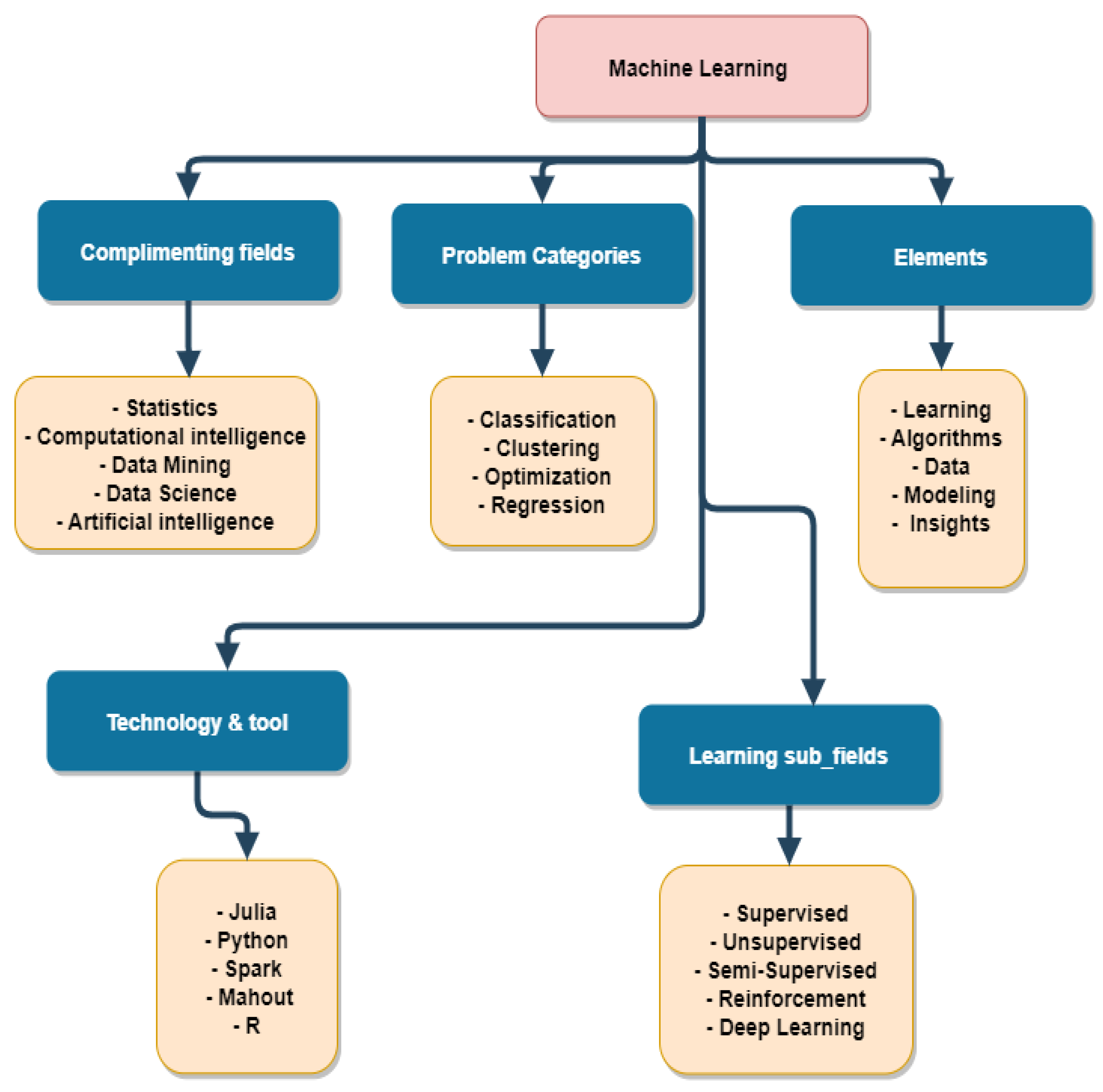
Figure 1. Machine Learning Parts.
Computation 11 00052 g001
Figure 2. The CNN Components.
Computation 11 00052 g002
Figure 3. A visual representation of the primary calculations.
Computation 11 00052 g003
Figure 4. Effects of different convolution matrices [21].
Computation 11 00052 g004
Figure 5. Stride 1, the filter windows move only one time for each connection.
Computation 11 00052 g005
Figure 6. The effect of stride in the output.
Computation 11 00052 g006
Figure 7. Zero-padding.
Computation 11 00052 g007
Figure 8. Pooling layer.
Computation 11 00052 g008
Figure 9. Function of Activation.
Computation 11 00052 g009
Figure 10. Fully-connected layer.
Computation 11 00052 g010
Figure 11. Forward and backpropagation in hidden CNN layers.
Computation 11 00052 g011
Figure 12. Regularization to CNN.
Computation 11 00052 g012
Figure 13. The process of object detection.
Computation 11 00052 g013
Table 1. A comparison between different popular CNNs Architecture.
Architecture NameLayersMain ContributionHighlightsStrengthGaps
LeNet
LeNet-5
[1998]
7 (5 Convolution + 2 FC)First popular CNN architectureRapidly deployable and effective at resolving small-scale image recognition issues
  • Utilized spatial correlation to decrease computation and parameter count
  • Automated discovery of feature hierarchy structures
Inadequate scaling to varied image classes; Filter sizes that are too large; Weak feature extraction
AlexNet [2012]8
(5 Convolution + 3 Fully Connected)
More depth and breadth than the LeNet-Employs Relu, dropout, and overlap Pooling-NVIDIA GTX 580 GPUs
Makes use of Dropout and ReLU
AlexNet is comparable to
LeNet-5, except it is more complex, has more filters per layer and employs stacked convolutional layers.
  • Low, middle, and high-level feature extraction utilizing large and tiny size filters on the early (5 × 5 and 11 × 11) and final (5 × 5 and 11 × 11) layers (3 × 3)
  • Implemented regularization in CNN
  • Commenced parallel usage of GPUs as an accelerator to address difficult architectures
Neurons in the first and second layers that are dormant
  • Aliasing artifacts in learned feature maps as a result of a large filter size
ZfNet [2014]8Conceptualization of middle levels
  • Illustrated parameter tweaking by displaying the output of intermediary layers.
  • Diminished the filter size and stride in the initial two layers of AlexNe
Further processing of information is necessary for visualization.
VGG [2014]16–19 (13–16 convolution + 3 FC-Homogeneous structure—Small kernel size.
-Enhanced depth, reduced filter size
The accuracy of a model is improved by employing small convolutional filters with dimensions of 3 3 in each layer.
  • Introduced the concept of an effective receptive field
  • Presented the concept of a simple and homogeneous topology
Implementation of computationally costly fully linked layers
GoogLeNet [2015]22 Convolution layers, 9 Inception modules-Presented the block concept-Separated the transform and merge notions
Increased depth, the block concept, a different filter size, and the concatenation concept
A deeper and broader architecture with various receptive field sizes and a number of extremely small convolutions.
  • Introduced the concept of applying mutiscale filters to layers
  • Introduced the concept of divide, transform, and merge
  • Reduced the number of parameters by the use of bottleneck layer, global average-pooling at the final layer, and sparse connections
  • Use of auxiliary classifiers to enhance convergence rate
Due to diverse topologies, parameter modification is arduous and time-consuming.
  • The useful information may be lost due to a representational bottleneck
Inception-V3 [2015]42 Convolution layers, 10 Inception modules
48
-Resolves the representational bottleneck issue—Change large-size filters to tiny-size filters
-Employs a tiny filter size and improved feature representation
Enhances the efficiency of a network.
The application of Batch Normalization expedites the training process. Inception-building elements are employed effectively to go deeper.
Utilized asymmetric filters and bottleneck layer to decrease the computational expense of deep designs
  • Complexity of the architectural design
  • Absence of uniformity
ResNet [2016]50 in ResNet-50, 101 in ResNet-101, 152 in
ResNet-152
-Identity mapping based on links—Long-term retention of knowledge.
Overfitting-resistant due to symmetry mapping-based skip connections
A unique design that features “skip connections” and extensive batch normalization.Reduces the error rate of deeper networks; introduces the concept of residual learning; mitigates the vanishing gradient problem
  • A slightly intricate structure
  • Degrades information of feature-map in feed forwarding
  • Excessive adaptation of hyperparameters for a specific task as a result of stacking identical modules
DenseNet
DenseNet-121
[2017]
117 Convolution layers, 3 Transition layers, and 1 Classification layer-Information transmission between layers
Blocks of layers; layers that are interconnected.
All layers are intimately connected to one another in a feed-forward fashion. It mitigates the problem of vanishing gradients and requires few parameters.
  • Added depth or cross-layer dimension
  • Ensures maximum data flow across network layers
  • Prevents relearning redundant feature-maps
  • Both low-level and high-level features are available to decision layers
Significant rise in parameters as a result of an increase in the number of feature-maps per layer
Table 2. A comparison between different Types of CNN.
ModelsTypes of CNNAdvantagesLimitations
Fast R-CNN
[2015]
Object detection
Two-stage framework
The properties of CNN are calculated in a single loop, making the detection of objects 25 times faster than the RCNN approach (an average of 20 s is required to study a picture).Using an external candidate region generator slows down the detection procedure.
Faster R-CNN
[2015]
Object detection
Two-stage framework
The RPN approach enables near-real-time object detection, around 0.12 s per image.Despite the algorithm’s effectiveness, it is too slow to be used in applications requiring real-time, such as driverless vehicles.
Mask R-CNN
[2017]
Object detection
Two-stage framework
When segmenting the objects in an image, the location of the objects becomes more exact.Its execution time is longer than that of the Faster-RCNN approach; hence, it cannot be implemented in real-time applications.
YOLO
[2015]
Object detection
One-stage framework
The efficiency of object localization enables its usage in real-time applications.The technique has trouble accurately detecting little items.
SSD
[2016]
Object detection
One-stage framework
YOLO and Faster R-CNN advantages are balanced with high detection speed and high object detection rate.Compared to the Fast-RCNN and Faster-RCNN algorithms, the object detection accuracy is less precise.
FCN
[2014]
Semantic segmentationObtaining a complete convolutional layer (without connected layer).Poor precision of feature maps and significant GPU utilization.
UNet
[2015]
Semantic segmentationThe structure has fewer parameters and is basically like the letter U. Appropriate for object detection in limited medical image samples.It is difficult to acquire uniform sub-sampling and up-sampling standards.
Disclaimer/Publisher’s Note: The statements, opinions and data contained in all publications are solely those of the individual author(s) and contributor(s) and not of MDPI and/or the editor(s). MDPI and/or the editor(s) disclaim responsibility for any injury to people or property resulting from any ideas, methods, instructions or products referred to in the content.