Abstract
The emergence of new embedded system technologies, such as IoT, requires the design of new lightweight cryptosystems to meet different hardware restrictions. In this context, the concept of Finite State Machines (FSMs) can offer a robust solution when using cryptosystems based on finite automata, known as FAPKC (Finite Automaton Public Key Cryptosystems), introduced by Renji Tao. These cryptosystems have been proposed as alternatives to traditional public key cryptosystems, such as RSA. They are based on composing two private keys, which are two FSMs and with the property of invertibility with finite delay to obtain the composed FSM , which is the public key. The invert process (factorizing) is hard to compute. Unfortunately, these cryptosystems have not really been adopted in real-world applications, and this is mainly due to the lack of profound studies on the FAPKC key space and a random generator program. In this paper, we first introduce an efficient algebraic method based on the notion of a testing table to compute the delay of invertibility of an FSM. Then, we carry out a statistical study on the number of invertible FSMs with finite delay by varying the number of states as well as the number of output symbols. This allows us to estimate the landscape of the space of invertible FSMs, which is considered a first step toward the design of a random generator.
1. Introduction
For centuries, cryptography has been used to ensure the privacy of sensitive information. Its evolution has been closely tied to military communication throughout history. However, in the Information Age, there is a growing demand for secure communication in both commercial and personal contexts. Before the introduction of public key cryptography, all ciphers relied on a shared secret key, meaning that both parties needed the same key to encrypt and decrypt messages. This requirement for exchanging a secret key beforehand became a crucial step in enabling secure communication.
The emergence of public key cryptosystems brought about a revolutionary change in the field of cryptography by streamlining the distribution of keys. Unlike traditional methods that involve sharing secret keys, this new approach allowed users to share their public key with others. The public key could be used by the sender to encrypt the message, but it could not be utilized for decryption. Instead, the recipient possessed a corresponding private key that remained confidential, and they used this key to decrypt the message. This breakthrough eliminated the need for key exchange and simplified the encryption process significantly.
The concept of public key cryptography was first proposed in 1976 by Hellman, Diffie, and Merkle. Two years later, Shamir, Rivest, and Adleman developed the RSA cryptosystem, which relies on the challenge of factoring large numbers. In 1985, Taher ElGamal introduced the ElGamal cryptosystem, which is based on the discrete logarithm problem. Additionally, in that same year, Victor Miller and Neal Koblitz separately introduced elliptic curve cryptography, which utilizes the discrete logarithm problem on elliptic curves. Elliptic curves, despite being more complex mathematically, offer faster operation and smaller key sizes while maintaining a similar level of security to other cryptosystems based on number theory problems. However, these systems are dependent on a small set of problems, making them potentially vulnerable.
In the late 1970s, Renji Tao and his research group proposed a series of Finite Automata Public Key Cryptosystems (FAPKCs) [1,2,3]. These systems utilize the challenge of inverting nonlinear Finite State Machines (FSMs) and factoring matrix polynomials over a field, instead of relying on number theory problems. FAPKCs have several advantages, including small key sizes, fast encryption and decryption processes, and the ability to be used for digital signatures. Furthermore, they can be implemented efficiently using logical operations, making them suitable for embedded hardware applications [2].
The private keys in FAPKCs are represented by two FSMs with memory, as shown in Figure 1. One is linear and the second is quasilinear [4]. These FSMs are combined using a special product in order to generate a nonlinear FSM, which is the public key. Currently, there is no known algorithm to invert nonlinear FSMs or factorize them, which remains an open problem. To invert the FSM public key, it is necessary to compute the inverses of its factors, a task made straightforward using the private key FSMs. Variants of FAPKCs exist, which differ in terms of the types of FSMs employed in private keys [5].
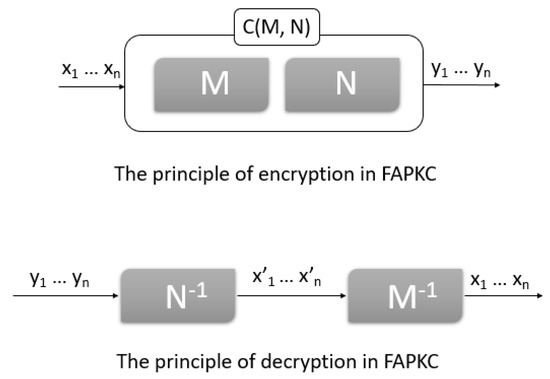
Figure 1.
An illustrative schema of an FAPKC.
Although some FAPKC schemes have been shown to be insecure [6], they are still considered a viable alternative to traditional cryptosystems. However, the study of FAPKCs has been hindered by the use of dry language in many papers, with results often lacking proofs and examples and referencing Chinese papers. Amorim et al. provided clarification and consolidation of existing research about FAPKCs in a series of papers [7,8,9,10] and a PhD thesis [4].
The invertibility of FSMs is a crucial concept in formal language theory and automata theory. Inverting a machine enables the reversal of its operation, which has numerous applications in various fields. In addition to cryptography, where FSMs are used as the basic concept for FAPKCs, the invertibility of FSMs has a broad range of applications that improve the performance of various systems. For example, they can be used to design systems that regulate and stabilize the behavior of complex systems [11], and they enable the reconstruction of original data from extracted features in pattern recognition [12]. In automata learning [13], they can generate counterexamples that guide the learning process.
To advance the development of efficient and secure cryptosystems, it is crucial to examine the space of invertible FSMs that serve as keys to FAPKCs. This investigation involves the study of the properties and behavior of these automata. By understanding the characteristics of these keys, cryptographers can design better algorithms and protocols that are more resistant to attacks and can protect sensitive information.
In [5], R. Tao introduced the concept of invertibility and weak-invertibility, also called injectivity, for various classes of FSMs. The invertibility property of an FSM implies that if it generates identical output sequences for two given input sequences, regardless of their initial states, then the first input symbols of the two input sequences will also be identical. On the other hand, weak-invertibility ensures that if an FSM produces identical output sequences for two given input sequences that originate from the same initial state, then the first input symbols of these sequences will also be identical. Therefore, it can be stated that if an FSM is invertible, it is also weak-invertible. The procedure to check these properties, as described by Tao [5], is based on the structure of the testing graph. By examining it, one can determine the invertibility and weak-invertibility of an FSM. A limitation arises when dealing with testing graphs that have a large number of vertices. Due to the increased complexity, it becomes crucial to employ a more efficient algorithm for determining whether the graph is loop-free. Our research aims to address this limitation by presenting a novel method that offers a computationally feasible solution for this task.
Building upon the work suggested by Amorim et al. [4,14], this study aims to further explore the landscape of invertible FSMs by presenting an approximate analysis of a general case. The research conducted by Amorim et al. focused on Linear FSMs, specifically investigating the statistical properties and count of weak-invertible (injective) Linear FSMs. Their study centered on the analysis of matrices, particularly the invariant factors of the transfer function matrix associated with linear FSMs. The results obtained from their research provided insights on the estimatation of the key space size of weak-invertible FSMs in cryptographic systems as well as on recurrence relations for counting canonical linear FSMs and approximating equivalence classes.
In contrast, our study introduces an efficient algebraic method to test the invertibility of FSMs with a finite delay, encompassing a broader scope beyond linear FSMs. By conducting experiments and analyzing invertible FSMs for general cases, we aim to provide a comprehensive understanding of their capabilities and limitations. Our research serves as a complementary contribution to the existing work by Amorim et al., as we delve into nonlinear FSMs and address the problem of invertibility in a more encompassing manner. The insights gained from our study highlight the promising potential of invertible FSMs as practical alternatives for secure key generation and cryptographic applications.
This paper is structured as follows: In Section 2, we introduce some preliminary notations and the basic definitions of Finite State Machines and graphs. In Section 3, we give a concise overview of the concept of invertibility with finite delay of Finite State Machines. In Section 4, we present a new efficient algebraic method for testing the invertibility of FSMs as well as several experimental results that allow us to give an estimation of the landscape of their space. Section 5 concludes the paper.
2. Preliminaries
In this paper, we present preliminary concepts and key findings on the topic of Finite State Machine (FSM) invertibility.
An alphabet is a finite set of symbols where . A word over is a finite sequence of symbols of length l.
The empty sequence, denoted by , represents a word of length . We define as the set of words of length n, where . Thus, . Furthermore, denotes the set of all finite words, obtained by the union of for . Additionally, represents the set of infinite words, composed of symbols , where .
2.1. Finite State Machines
Finite State Machines (FSMs) have found widespread use as models for various types of systems in fields, such as sequential circuits, program development (e.g., lexical analysis and pattern matching), and communication protocols [15,16,17,18]. In this paper, we specifically focus on Mealy machines, which are deterministic machines that generate outputs during state transitions after receiving inputs.
Definition 1.
A Finite State Machine is represented by a quintuple , where denotes the input alphabet, denotes the output alphabet, denotes the set of states, defines the state transition function, and represents the output function.
Let be a Finite State Machine (FSM). The state transition function δ and the output function λ can be extended to finite words in recursively using the following definitions:
where , , and . Similarly, the output function λ can be extended to infinite words in . From these definitions, it follows that for any , , and , the output of λ for can be computed as .
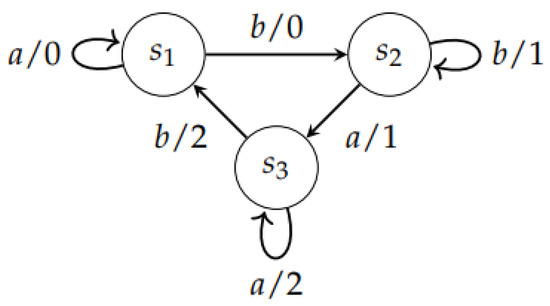
Example 1.
The Finite State Machine with:
- is represented by the diagram in Figure 2.
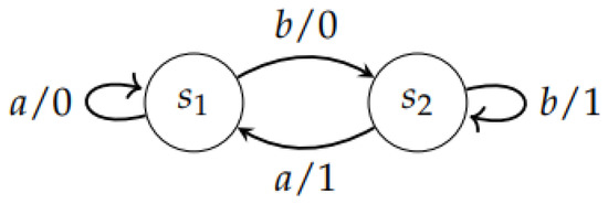 Figure 2. The Finite State Machine .
2.2. Graphs
Let be a directed cycle-free graph, where V represents the vertex set, and denotes the arc set. If V is an empty set, the graph is referred to as an empty graph. The elements in V are referred to as vertices, while the elements in are referred to as arcs. Let :
- -
- If v is isolated, then .
- -
- If v has no incoming arc and it has at least one outgoing arc, then .
- -
- If v has at least one incoming arc and at least one outgoing arc, then = Maximum .
- -
- The level of the graph is = Maximum .
- -
- If is the empty graph, then = .
Example 2.
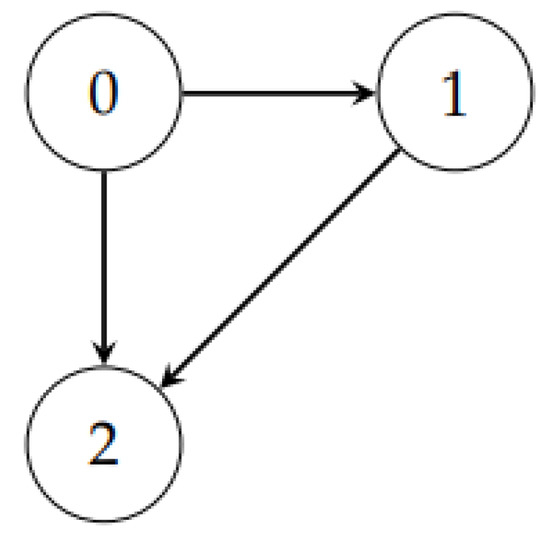
Computing the level of a directed cycle-free graph (Figure 3)
Figure 3.
A directed cycle-free graph.
The level of this graph is 1.
Remark 1.
Let be a cycle-free directed graph of level l. Then, the maximum length of a path in is .
3. The Concept of Invertibility of Finite State Machines
In this section, we recall the concept of invertibility with finite delay of an FSM, where , as well as the classical testing method based on graph theory for the invertibility property of an FSM. For more details, refer to [5].
3.1. The Invertibility with Finite Delay of an FSM
An FSM is said to be invertible if for any state in the set of states and any output sequence, the input sequence that produced the output sequence can be uniquely determined. An FSM is considered invertible with some delay if, for any state and any sequence of input symbols , the output sequence , generated by , uniquely determines the input symbol . This means that if produces identical output sequences for a given two input sequences, then their first input symbols are also identical. The delay is a non-negative integer that represents the number of input symbols used to determine the output symbol. The formal definitions of both are as follows:
Definition 2.
A Finite State Machine is considered to be invertible if
.
This means that for every pair of states and every pair of infinite words , if the output generated by the FSM is the same for both state–input pairs, i.e., , then the infinite words α and must be identical.
Definition 3.
A Finite State Machine is considered to be τ-invertible or invertible with finite delay τ, where , if
with , if , then .
This implies that for any pair of states and any sequence of inputs with , if the outputs generated by the FSM are the same for both state–input sequences, i.e., , then the initial inputs and must be identical.
It is evident that if is invertible with a delay of , then is also invertible. The reverse statement is also true (refer to [5]).
Example 3.
Let us consider the FSM presented in Example 1. is invertible with a delay of 1, since we have for all input sequences of length 2:
Example 4.
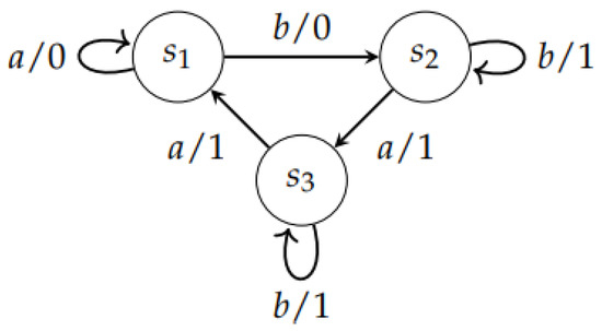
The FSM induced by the diagram in Figure 4 is not invertible with a delay of 1, since and .
Figure 4.
The Finite State Machine .
Example 5.
The FSM induced by the diagramis invertible with a delay of 1 (Figure 5). To prove this, we have to compute the outputs for all states with all input sequences of :
Figure 5.
The Finite State Machine .
3.2. Graph-Based Method for Testing the Invertibility of an FSM
Let us recall some important properties of the invertibility with finite delay of an FSM, as well as the classical method for testing these properties.
Let be an FSM. Let us define the testing graph of as follows:
.
- (a)
- if , then:- The vertex set V of is the minimal subset of , which verifies:
- (a)
- ,
- (b)
- if and , , then .
- The arc set of is the set of all arcs , such that:- (a)
- ,
- (b)
- , where .
- (b)
- if then is the empty graph, .
In other words, the graph is constructed by forming a graph of the state transitions and output values based on the conditions described above. The vertices in the graph represent pairs of states that have the same output value for any input symbol, and the arcs represent the transition from one pair of states to another pair of states with the same output value. The graph is constructed to minimize the number of vertices and to satisfy the conditions for the vertices and arcs as described in the conditions.
Theorem 1
(Theorem 1.4.1, [5]). Let be a Finite State Machine. is invertible if and only if has no circuit. Moreover, if has no circuit and the level of is , then is invertible with a delay of and not invertible with a delay of τ for any .
Corollary 1.
If is invertible, then exists, such that is invertible with a delay of τ.
Example 6. 
Let us define the testing graph of defined in Example 4.
is the set of pairs of states that have the same output value for any two distinct input symbols, a and b. It is calculated by applying the transition function δ and the output function λ to each state s and to the input symbols a and b.
V is the vertex set of the graph . It is a minimal subset of the set of state pairs that have the same output value for any input symbol. To form V, we start with and keep adding state pairs that have the same output value and are reachable from other state pairs in V. Using the information provided in the example and :
Γ is the arc set of the graph . It consists of all arcs connecting pairs of state pairs that have the same output value for any input symbol. To form Γ, we connect each state pair in V to its reachable state pairs that have the same output value:
Note that this is the set of arcs connecting the state pairs in V. The graph is represented by:
The testing graph has a circuit; therefore, it is not invertible.
Example 7. 

The FSM is represented by the following diagram:
The graph can be constructed as follows:
The graph is loop-free, and the maximum length of a path is 1; therefore, is invertible with a delay of .
When the number of vertices is very large in a testing graph , it is important to have a more efficient algorithm to decide whether it is loop-free. In the next section, we present one such algorithm that can be easily executed by a computer.
4. A New Algebraic Method for Testing the Invertibility of FSMs
In this section, we introduce an efficient algorithm for testing and computing the delay of invertibility of a given FSM. We also conduct some experiments in order to produce an estimation of the landscape of the set of invertible FSMs. Our method is based on the notion of the testing table, instead of the testing graph of an FSM, which allows us to conduct a fast test using iterative zero-matrix reduction.
4.1. Algebraic Method for Testing the Invertibility of an FSM
The major tools used in the proposed method are the testing table and its corresponding connection matrix.
Definition 4.
The testing table associated with an FSM is an application defined by two steps, as follows:
- , such that and , for all .
- for all , we define: , such that , for all .
Note that, in Definition 4, we consider for all . Then, the testing table has rows and columns. To simplify the notation, in the next section, we note that .
By construction, the testing table is defined in two steps. First, the table entries are the successor’s pairs of states of a given pair of states’ row index if they have outgoing transitions with the same output symbol and different input symbols. Then, from the resulting pairs of states in the first step, the testing table entries are completed by the set of their successor’s pairs if they have outgoing transitions with the same output symbol.
Definition 5.
The connection matrix associated with a testing table of an FSM is an matrix, where , whose rows and columns are labeled by the set of pair of states and the th entry is 1 if exists, such that , or 0 otherwise.
Based on its connection matrix, the checking of the invertibility of an FSM is performed with Algorithm 1.
Here is a step-by-step description of the testing algorithm:
- Construct the corresponding connection matrix based on the testing table.
- Delete all rows that consist of only zeroes in every position, and remove the corresponding columns. If there are no rows with all zeroes, proceed to step 4.
- Repeat step 2 until there are no more rows with all zeroes.
- If the matrix still has rows or columns remaining after the iterations, this indicates that the graph is not loop-free; otherwise, if the matrix has completely vanished, it means that the graph is loop-free.
| Algorithm 1: Reduction of a connection matrix. |
 |
From a given connection matrix of a testing table of an FSM Algorithm 1 eliminates all rows that consist entirely of zeroes as well as their corresponding columns and repeats this process until no more rows can be eliminated. If the resulting matrix is empty (i.e., it has no rows or columns), the FSM associated with the input connection matrix is invertible.
It is important to note that if there are two or more rows in the matrix that contain only zeroes in all of their positions, then these rows and their corresponding columns must be removed together, and this procedure will be counted as a single iteration.
In summary, the algorithm checks for rows of zeroes in the matrix and removes them, updating the matrix until no more rows of zeroes are found. The number of iterations required to remove all rows of zeroes represents the finite delay . If the matrix has vanished, then M is invertible with a finite delay ; otherwise, it is not invertible. (A “vanished” matrix has no columns or rows.)
Example 8.

Let us consider the FSM defined in Example 7. The testing table in Table 1 of is as follows:
Table 1.
The testing table of .
The corresponding connection matrix is as follows:
In this matrix, the rows and columns are labeled with the state pairs. The cells of the matrix represent the output symbol associated with the transition from the current state pair to the next state pair. The output symbol is represented by 0 or 1, where 0 represents no transition and 1 represents a transition.
First, we remove the rows labeled , , and their corresponding columns. After that, we repeat the application of this step, which will result in the deletion of the row labeled .
The next step results in the matrix disappearing entirely. Consequently, is invertible with a delay of , as is already shown in Example 7.
Theorem 2.
Algorithm 1 checks the invertibility of an FSM and computes its delay in a time period of .
Proof.
Let us consider an FSM . Suppose that is not invertible and Algorithm 1 produces an empty connection matrix. By the construction of the connection matrix , there are rows indexed by the pairs of states from step 1 in the corresponding testing table. This means that exists, such that and . Since is not invertible, two input sequences and exist, such that . Suppose now that , and , for all . We have
- and ,
- , for all .
The connection matrix is as follows:
According to Algorithm 1, the ones are eliminated when the corresponding columns correspond to an empty row. In our case, the matrix cannot be reduced. Consequently, is invertible.
To prove the sufficiency condition, assume that Algorithm 1 produces a nonempty matrix. Without a loss of generality, we can consider a produced matrix with the previous matrix form. Then, two input sequences and exist, such that for some , we have and . Then, the associated FSM is not invertible.
The time complexity of Algorithm 1 depends on the number of rows in the connection matrix. Since there are rows and columns, Algorithm 1 runs in the worst case scenario of a time period of . Thus, the Theorem is proved. □
4.2. Experimentation and Results
This section aims to present an estimation of the landscape of invertible FSMs through the proposed algebraic testing method and randomized statistical sampling.
Theorem 3.
The number of Finite State Machines with n states, i input alphabet symbols, and o output alphabet symbols is equal to .
Proof.
Let us assume that we have an FSM with n states, i input alphabet symbols, and o output alphabet symbols. First, consider the input side of the FSM. There are i possible input symbols and n possible states. Since the FSM is complete, for each state, there must be a transition defined for every input symbol in the alphabet. Therefore, the number of possible transitions from each state is equal to . Therefore, there are possible transition tables for the input side of the FSM. Next, consider the output side of the FSM. There are o possible output symbols that can be associated with each transition in the input side of the FSM. Therefore, there are possible transitions for each state in the output side of the FSM. Finally, to determine the total number of FSMs, we need to consider all possible combinations of transitions with input symbols and output symbols. Thus, the total number of possible FSMs is . □
Table 2 summarizes the total number of considered FSMs in our experiments when for a different number of states n and output alphabet size o in .
Table 2.
The total number of FSMs when .
It should be noted that we consider the input symbols to be in the binary alphabet, since real-world data are typically encoded in binary format.
The algorithm described in this paper was implemented in Java, and its detailed description is available in the repository [19]. A series of experiments were conducted using these implementations, which led to significant findings.
We exhibit the number of -invertible classes for and a given value of , while the n and range are and , respectively.
For each triple of structural parameters i, o, and n, we uniformly and randomly generated a sample of 20000 FSMs. We computed the number of -invertible FSMs in these samples.
The graphs presented in Figure 6 represent the number of -invertible FSMs that can be built with a certain number of states and output symbols. They were generated using the approximate values obtained from the tables in Appendix A.
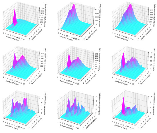
Figure 6.
Approximate values for the number of -invertible FSMs when i = 2.
The x-axis shows the number of states, ranging from 2 to 20, and the y-axis shows the number of output symbols, ranging from 2 to 8. The z-axis represents the number of invertible FSMs that can be constructed for each combination of a number of states and output symbols. The surface plot shows a peak where the number of invertible FSMs is the highest. The plot shows that the number of invertible FSMs generally increases with the number of states and outputs. However, the rate of increase appears to decrease as the number of states and output symbols increases.
Overall, these plots provide a clear visualization of the relationship between the number of states, number of outputs, and number of invertible FSMs, with the peak indicating the most favorable conditions for constructing invertible FSMs.
The heatmap in Figure 7 shows the number of invertible FSMs for different combinations of the number of states and output symbols when the number of input symbols is fixed at 2.
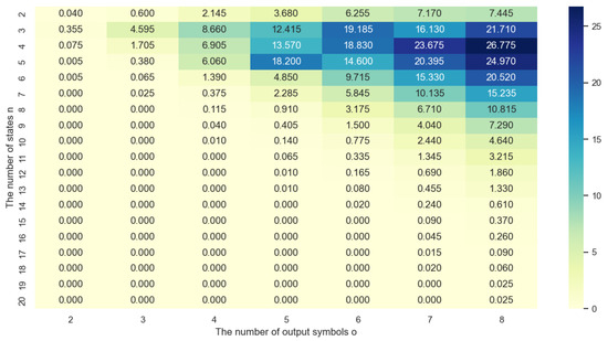
Figure 7.
Heatmap showing the approximate percentage values of invertible FSMs when i = 2.
The number of states is presented on the y-axis, while the number of output symbols is presented on the x-axis. The cells of the heatmap represent the total number of invertible FSMs for the corresponding combination of the number of states and output symbols.
From the heatmap, the main observation is that there is an increase in the number of invertible FSMs when the number of states n is much smaller than the number of output symbols o i.e., . This is principally due to the fact that an increase in the number of output symbols expands the number of potential transitions between states, consequently leading to a higher number of possible FSMs. Conversely, as the number of states rises relative to the number of outputs, the heatmap demonstrates that the number of invertible Finite State Machines decreases. Notably, when the number of states greatly exceeds the number of outputs, the count of invertible FSMs reaches zero.
From various experiments involving the estimation of the landscape of invertible FSMs, it has been observed that the number of invertible FSMs can grow exponentially under certain conditions. This characteristic renders them a viable solution for creating efficient and lightweight keys that offer resistance to brute force attacks in any cryptosystem. Invertible FSMs have been shown to be a promising alternative to traditional cryptographic methods, and they can offer several advantages in terms of security, efficiency, and ease of implementation [20]. However, further research and testing may be necessary to fully explore the potential of invertible FSMs for different cryptographic applications.
5. Conclusions
The construction of invertible finite automata has two critical applications in the field of cryptography: Firstly, they are utilized to generate encryption and signature keys in FAPKCs. Secondly, they can be used to attack existing cryptographic systems based on finite automata theory. In this paper, we presented an efficient algebraic algorithm that allows us to check the invertibility of FSMs with some finite delay. Then, we presented an estimation of the landscape of invertible FSMs through some experiments conducted for general cases. Our study was conducted as suggested by [14] and shows that invertible FSMs are promising alternatives to conventional cryptographic methods and can potentially provide a practical solution for creating efficient and lightweight keys that offer resistance to brute force attacks. Overall, the study of the invertibility of finite FSMs is an active area of research with both theoretical and practical implications.
Author Contributions
Conceptualization, Z.L., H.K. and F.O.; Methodology, Z.L. and F.O.; Software, Z.L.; Validation, F.O.; Formal analysis, Z.L., H.K. and F.O.; Investigation, Z.L. and F.O.; Data curation, Z.L. and F.O.; Writing—original draft, Z.L.; Writing—review & editing, Z.L., H.K. and F.O.; Visualization, Z.L.; Supervision, H.K. and F.O.; Project administration, F.O. All authors have read and agreed to the published version of the manuscript.
Funding
This research received no external funding.
Conflicts of Interest
The authors declare no conflict of interest.
Appendix A
Table A1.
Approximate number values for and .
Table A1.
Approximate number values for and .
| n | |||
|---|---|---|---|
| 2 | 0 | 8 | 0 |
| 3 | 0 | 71 | 0 |
| 4 | 0 | 14 | 1 |
| 5 | 0 | 1 | 0 |
| 6 | 0 | 1 | 0 |
| 7 | 0 | 0 | 0 |
| 8 | 0 | 0 | 0 |
| 9 | 0 | 0 | 0 |
| 10 | 0 | 0 | 0 |
Table A2.
Approximate number values for and .
Table A2.
Approximate number values for and .
| n | |||||
|---|---|---|---|---|---|
| 2 | 0 | 120 | 0 | 0 | 0 |
| 3 | 9 | 760 | 136 | 14 | 0 |
| 4 | 19 | 215 | 80 | 25 | 2 |
| 5 | 6 | 39 | 25 | 6 | 0 |
| 6 | 0 | 4 | 8 | 1 | 0 |
| 7 | 0 | 2 | 3 | 0 | 0 |
| 8 | 0 | 0 | 0 | 0 | 0 |
| 9 | 0 | 0 | 0 | 0 | 0 |
| 10 | 0 | 0 | 0 | 0 | 0 |
Table A3.
Approximate number values for and .
Table A3.
Approximate number values for and .
| n | |||||||||
|---|---|---|---|---|---|---|---|---|---|
| 2 | 0 | 429 | 0 | 0 | 0 | 0 | 0 | 0 | 0 |
| 3 | 5 | 1424 | 292 | 11 | 0 | 0 | 0 | 0 | 0 |
| 4 | 45 | 821 | 416 | 82 | 16 | 0 | 1 | 0 | 0 |
| 5 | 605 | 34 | 236 | 220 | 71 | 32 | 9 | 2 | 1 |
| 6 | 33 | 76 | 97 | 39 | 24 | 5 | 2 | 2 | 0 |
| 7 | 13 | 13 | 22 | 15 | 5 | 2 | 4 | 1 | 0 |
| 8 | 3 | 3 | 5 | 7 | 4 | 0 | 0 | 1 | 0 |
| 9 | 2 | 0 | 0 | 0 | 1 | 2 | 3 | 0 | 0 |
| 10 | 0 | 0 | 0 | 0 | 1 | 0 | 1 | 0 | 0 |
| 11 | 0 | 0 | 0 | 0 | 0 | 0 | 0 | 0 | 0 |
| 12 | 0 | 0 | 0 | 0 | 0 | 0 | 0 | 0 | 0 |
Table A4.
Approximate number values for and .
Table A4.
Approximate number values for and .
| n | |||||||||
|---|---|---|---|---|---|---|---|---|---|
| 2 | 0 | 736 | 0 | 0 | 0 | 0 | 0 | 0 | 0 |
| 3 | 0 | 2168 | 311 | 4 | 0 | 0 | 0 | 0 | 0 |
| 4 | 42 | 1781 | 766 | 104 | 19 | 2 | 0 | 0 | 0 |
| 5 | 1820 | 73 | 855 | 646 | 194 | 41 | 4 | 4 | 3 |
| 6 | 72 | 291 | 381 | 165 | 42 | 13 | 6 | 0 | 0 |
| 7 | 47 | 87 | 179 | 84 | 40 | 13 | 4 | 2 | 1 |
| 8 | 22 | 30 | 50 | 49 | 22 | 5 | 2 | 1 | 1 |
| 9 | 11 | 10 | 12 | 24 | 16 | 4 | 1 | 2 | 1 |
| 10 | 9 | 1 | 6 | 3 | 5 | 4 | 0 | 0 | 0 |
| 11 | 3 | 0 | 1 | 4 | 1 | 2 | 2 | 0 | 0 |
| 12 | 1 | 0 | 0 | 1 | 0 | 0 | 0 | 0 | 0 |
| 13 | 1 | 0 | 0 | 0 | 1 | 0 | 0 | 0 | 0 |
| 14 | 0 | 0 | 0 | 0 | 0 | 0 | 0 | 0 | 0 |
| 15 | 0 | 0 | 0 | 0 | 0 | 0 | 0 | 0 | 0 |
Table A5.
Approximate number values for and .
Table A5.
Approximate number values for and .
| n | |||||||||
|---|---|---|---|---|---|---|---|---|---|
| 2 | 0 | 1251 | 0 | 0 | 0 | 0 | 0 | 0 | 0 |
| 3 | 3 | 3436 | 389 | 9 | 0 | 0 | 0 | 0 | 0 |
| 4 | 35 | 2731 | 892 | 103 | 5 | 0 | 0 | 0 | 0 |
| 5 | 65 | 1578 | 984 | 234 | 52 | 5 | 2 | 0 | 0 |
| 6 | 83 | 748 | 766 | 256 | 70 | 13 | 6 | 1 | 0 |
| 7 | 75 | 291 | 513 | 209 | 57 | 20 | 1 | 2 | 1 |
| 8 | 45 | 99 | 242 | 158 | 64 | 17 | 6 | 3 | 1 |
| 9 | 34 | 17 | 111 | 80 | 31 | 18 | 4 | 4 | 1 |
| 10 | 26 | 12 | 42 | 47 | 23 | 4 | 1 | 0 | 0 |
| 11 | 13 | 3 | 16 | 19 | 11 | 3 | 1 | 0 | 1 |
| 12 | 7 | 0 | 1 | 10 | 7 | 3 | 1 | 3 | 0 |
| 13 | 9 | 0 | 1 | 3 | 1 | 2 | 0 | 0 | 0 |
| 14 | 2 | 0 | 0 | 1 | 1 | 0 | 0 | 0 | 0 |
| 15 | 0 | 0 | 0 | 0 | 0 | 0 | 0 | 0 | 0 |
| 16 | 0 | 0 | 0 | 0 | 0 | 0 | 0 | 0 | 0 |
Table A6.
Approximate number values for and .
Table A6.
Approximate number values for and .
| n | |||||||||
|---|---|---|---|---|---|---|---|---|---|
| 2 | 0 | 1434 | 0 | 0 | 0 | 0 | 0 | 0 | 0 |
| 3 | 3 | 2962 | 259 | 2 | 0 | 0 | 0 | 0 | 0 |
| 4 | 27 | 3728 | 885 | 88 | 7 | 0 | 0 | 0 | 0 |
| 5 | 68 | 2597 | 1135 | 248 | 29 | 2 | 0 | 0 | 0 |
| 6 | 92 | 1402 | 1191 | 295 | 74 | 8 | 3 | 1 | 0 |
| 7 | 77 | 675 | 880 | 311 | 68 | 13 | 3 | 0 | 0 |
| 8 | 81 | 305 | 587 | 268 | 77 | 20 | 3 | 1 | 0 |
| 9 | 75 | 121 | 341 | 204 | 52 | 12 | 3 | 0 | 0 |
| 10 | 52 | 36 | 193 | 126 | 52 | 19 | 8 | 2 | 0 |
| 11 | 31 | 9 | 111 | 75 | 29 | 11 | 1 | 1 | 1 |
| 12 | 19 | 2 | 41 | 43 | 23 | 6 | 4 | 0 | 0 |
| 13 | 19 | 1 | 22 | 28 | 16 | 1 | 1 | 2 | 1 |
| 14 | 10 | 0 | 10 | 12 | 8 | 5 | 2 | 1 | 0 |
| 15 | 5 | 0 | 6 | 1 | 3 | 2 | 1 | 0 | 0 |
| 16 | 2 | 0 | 2 | 4 | 0 | 1 | 0 | 0 | 0 |
| 17 | 1 | 0 | 0 | 2 | 0 | 0 | 0 | 0 | 0 |
| 18 | 1 | 0 | 0 | 1 | 0 | 0 | 1 | 1 | 0 |
| 19 | 0 | 0 | 0 | 0 | 0 | 0 | 0 | 0 | 0 |
| 20 | 0 | 0 | 0 | 0 | 0 | 0 | 0 | 0 | 0 |
Table A7.
Approximate number values for and .
Table A7.
Approximate number values for and .
| n | |||||||||
|---|---|---|---|---|---|---|---|---|---|
| 2 | 0 | 1489 | 0 | 0 | 0 | 0 | 0 | 0 | 0 |
| 3 | 2 | 4009 | 327 | 4 | 0 | 0 | 0 | 0 | 0 |
| 4 | 22 | 4353 | 891 | 80 | 9 | 0 | 0 | 0 | 0 |
| 5 | 48 | 3417 | 1295 | 196 | 33 | 4 | 1 | 0 | 0 |
| 6 | 66 | 2259 | 1369 | 339 | 61 | 9 | 1 | 0 | 0 |
| 7 | 78 | 1284 | 1197 | 392 | 76 | 19 | 1 | 0 | 0 |
| 8 | 95 | 630 | 957 | 350 | 105 | 21 | 4 | 1 | 0 |
| 9 | 91 | 308 | 631 | 321 | 84 | 16 | 6 | 1 | 0 |
| 10 | 79 | 103 | 410 | 235 | 73 | 22 | 6 | 0 | 0 |
| 11 | 61 | 43 | 263 | 189 | 63 | 16 | 7 | 0 | 1 |
| 12 | 42 | 16 | 133 | 119 | 42 | 18 | 2 | 0 | 0 |
| 13 | 34 | 10 | 78 | 100 | 31 | 11 | 0 | 1 | 0 |
| 14 | 17 | 2 | 29 | 40 | 23 | 8 | 1 | 1 | 0 |
| 15 | 12 | 1 | 20 | 29 | 9 | 3 | 0 | 0 | 0 |
| 16 | 9 | 1 | 12 | 15 | 5 | 8 | 2 | 0 | 0 |
| 17 | 7 | 0 | 2 | 4 | 3 | 2 | 0 | 0 | 0 |
| 18 | 3 | 0 | 0 | 4 | 2 | 2 | 1 | 0 | 0 |
| 19 | 0 | 0 | 1 | 2 | 1 | 1 | 0 | 0 | 0 |
| 20 | 1 | 0 | 0 | 1 | 2 | 1 | 0 | 0 | 0 |
References
- Tao, R.; Chen, S.; Chen, X. Fapkc3: A new finite automaton public key cryptosystem. J. Comput. Sci. Technol. 1997, 12, 289. [Google Scholar] [CrossRef]
- Tao, R.; Chen, S. A variant of the public key cryptosystem fapkc3. J. Netw. Comput. Appl. 1997, 20, 283–303. [Google Scholar] [CrossRef]
- Tao, R.; Chen, S. The generalization of public key cryptosystem fapkc4. Chin. Sci. Bull. 1999, 44, 784–790. [Google Scholar] [CrossRef]
- Amorim, I. Linear Finite Transducers towards a Public Key Cryptographic System. Ph.D. Thesis, Faculdade de Ciências da Universidade do Porto, Porto, Portugal, 2016. [Google Scholar]
- Renji, T. Finite Automata and Application to Cryptography; Springer: Chicago, IL, USA, 2008. [Google Scholar]
- Bao, F.; Igarashi, Y. Break Finite Automata Public Key Cryptosystem; Springer: Berlin, Heidelberg, 1995; pp. 147–158. [Google Scholar]
- Amorim, I.; Machiavelo, A.; Reis, R. Formal power series and the invertibility of finite linear transducers. In Proceedings of the Non-Classical Models for Automata and Applications, Fribourg, Switzerland, 23–24 August 2022; pp. 33–48. [Google Scholar]
- Amorim, I.; Machiavelo, A.; Reis, R. Counting equivalent linear finite transducers using a canonical form. In Proceedings of the 19th International Conference on Implementation and Application of Automata, CIAA 2014, Giessen, Germany, 30 July–2 August 2014; Springer: Berlin/Heidelberg, Germany, 2014; pp. 70–83. [Google Scholar]
- Amorim, I.; Machiavelo, A.; Reis, R. On the invertibility of finite linear transducers. Rairo-Theor. Inform. Appl. 2014, 48, 107–125. [Google Scholar] [CrossRef]
- Amorim, I.; Machiavelo, A.; Reis, R. Statistical study on the number of injective linear finite transducers. arXiv 2014, arXiv:1407.0169. [Google Scholar]
- Wagner, F.; Schmuki, R.; Wagner, T. Wolstenholme. Modeling Software with Finite State Machines: A Practical Approach; CRC Press: Boca Raton, FL, USA, 2006. [Google Scholar]
- Khotanzad, A.; Hong, Y.H. Invariant image recognition by Zernike moments. IEEE Trans. Pattern Anal. Mach. Intell. 1990, 12, 489–497. [Google Scholar] [CrossRef]
- Cassel, S.; Howar, F.; Jonsson, B.; Steffen, B. Active learning for extended finite state machines. Form. Asp. Comput. 2016, 28, 233–263. [Google Scholar] [CrossRef]
- Amorim, I.; Machiavelo, A.; Reis, R. On the Number of Linear Finite Transducers. Int. J. Found. Comput. Sci. 2015, 26, 873–893. [Google Scholar] [CrossRef]
- Chow, T.S. Testing software design modeled by finite-state machines. IEEE Trans. Softw. Eng. 1978, SE-4, 178–187. [Google Scholar] [CrossRef]
- Friedman, A.D.; Menon, P.R. Fault Detection in Digital Circuits; Prentice-Hall, Inc.: Englewood Cliffs, NJ, USA, 1971. [Google Scholar]
- Sethi, A.V.A.R.; Ullman, J.D. Compilers: Principles, Techniques, and Tools Reading; Addison-Wksley: Boston, MA, USA, 1986. [Google Scholar]
- Bolzmann, G.J. Design and Validation of Protocols; Prentice-Hall: Englewood Cliffs, NJ, USA, 1990. [Google Scholar]
- The Source Code for the Algorithm. Available online: https://github.com/ZinebLotfi/InvertiblesFSMs (accessed on 23 June 2023).
- Abubaker, S.; Wu, K. DAFA—A Lightweight DES Augmented Finite Automaton Cryptosystem. In Security and Privacy in Communication Networks, Proceedings of the 8th International ICST Conference, SecureComm 2012, Padua, Italy, 3–5 September 2012; Keromytis, A.D., Di Pietro, R., Eds.; Lecture Notes of the Institute for Computer Sciences, Social Informatics and Telecommunications Engineering; Springer: Berlin, Heidelberg, 2013; Volume 106. [Google Scholar]


Disclaimer/Publisher’s Note: The statements, opinions and data contained in all publications are solely those of the individual author(s) and contributor(s) and not of MDPI and/or the editor(s). MDPI and/or the editor(s) disclaim responsibility for any injury to people or property resulting from any ideas, methods, instructions or products referred to in the content. |
© 2023 by the authors. Licensee MDPI, Basel, Switzerland. This article is an open access article distributed under the terms and conditions of the Creative Commons Attribution (CC BY) license (https://creativecommons.org/licenses/by/4.0/).