Abstract
We propose two accurate and efficient spectral collocation techniques based on a (novel) domain-splitting strategy to handle a nonlinear fractional system consisting of three ODEs arising in financial modeling and with chaotic behavior. One of the major numerical difficulties in designing traditional spectral methods is in the handling of model problems on a long computational domain, which usually yields to loss of accuracy. One remedy is to split the underlying domain and apply the spectral method locally in each subdomain rather than on the global domain of interest. To treat the chaotic financial system numerically, we use the generalized version of modified Bessel polynomials (GMBPs) in the collocation matrix approaches along with the domain-splitting strategy. Whereas the first matrix collocation scheme is directly applied to the financial model problem, the second one is a combination of the quasilinearization method and the direct first numerical matrix method. In the former approach, we arrive at nonlinear algebraic matrix equations while the resulting systems are linear in the latter method and can be solved more efficiently. A convergence theorem related to GMBPs is proved and an upper bound for the error is derived. Several simulation outcomes are provided to show the utility and applicability of the presented matrix collocation procedures.
1. Introduction
There has been a great deal of interest in working with nonlinear ordinary differential equations (ODEs) and dynamical systems over the past decades. Diverse physical as well as nonphysical phenomena including economical, epidemiological, and biological models belong to these category. Among others, nonlinear systems with chaotic behavior are of particularly of interest. Chaos theory of nonlinear dynamics is a branch of mathematical science that deals with highly complex systems, where small changes now in their inputs cause large changes in their outputs later [1]. The notion of chaos was first introduced to the modern world by Edward Lorenz in 1972 with conceptualization of “Butterfly Effect”. By understanding this theory we are able to predict the behavioral representation of a complex system more accurately. Chaotic systems are unstable since they tend not to resist any outside disturbances but instead react in significant manner. As a meteorologist, Lorenz developed a mathematical model for the air movement in the atmosphere. It caused various differences in the outcome of the given model. In this manner he discovered the principle of sensitive dependence on initial conditions, which is now considered as a key element in any chaotic system [2]. Indeed, systems with chaotic behavior are common in nature and diverse real-life phenomena can also be classified in the framework of a chaotic system. Beside of their appearance in meteorology, they can be found also in solar system, chemical reactions, climate dynamic, population dynamic, economics, and so on.
In the economic setting, Ma and Chen [3,4] were one of the pioneering who studied and analyzed the chaotic economic systems. The study of memory effects and fractional-order derivative on a chaotic financial system was given by Chen [5]. The concept of fractional calculus provides more insight in predicting the behavior of complex dynamical systems especially those with chaotic characteristics, see [6]. Various fractional order systems with chaos have been considered in literature such as Chua [7], Chen [8], Rössler [9], Lorentz [10] to name a few. Finding the exact or analytical solutions of the most fractional-order systems cannot be possible. Alternately, the researchers have been tried to develop effective semi-analytical as well as numerical procedures to deal with such systems of fractional order. Among diverse existing proposed methods, we refer to the recent published works including the spectral collocation approaches [11,12,13], the fractional Adams-Bashforth approach [14], the residual power series method and Laplace technique [15], the variational iteration scheme [16], and the wavelet technique [17] to name a few.
The main objective of the current research is to investigate a real-life model arising in the financial market. The model equation consists of three differential equations with quadratic nonlinearities given by [5]
where and for are constants. Here, denotes the saving amount rate, represents the costs per investment, and shows the elasticity of demand of commercial markets. In the model (1) by we denote the fractional derivative operator of order in the sense of Liouville–Caputo (LC). Let , and be given real numbers. The supplemented initial conditions are as follow
It should be emphasized that the dynamic analysis and chaotic intrinsic nature of the financial system (1) have already been investigated by researchers, see cf. [5].
Based on our knowledge, only a few works have been proposed to solve the system (1) numerically. The Adams-Bashforth-Moulton scheme used in [18] to deal with the variable-order fractional counterpart of (1). The integer-order of the above model solved by a robust spectral Chebyshev method [19]. The fractional-order of model (1) in the sense of both Caputo and Atangana-Baleanu-Caputo (ABC) derivatives considered in [20] and solved by the modified homotopy analysis transform method. They also proved the existence and uniqueness of the solutions based on Picard-Lindelof’s approach. The variable-order of the underlying model in the sense of ABC derivative invsetiagted in [21]. A computational stochastic approach based on the artificial neural networks introduced recenlty in [22]. Furthermore, the authors in [23] proposed a new robust nonlinear controller that stabilizes the chaotic finance system (1). Some other financial models related to (1) with some proposed approximate methods were given in [24,25,26,27].
In this work, we solve the nonlinear system (1) with two spectral collocation approaches based on (novel) modified Bessel functions. To preserve the high accuracy of the proposed methods on a long computational domain, we further employ the domain-splitting methodology. In the first and direct collocation procedure, we convert the financial model into an algebraic system of nonlinear equations. On the other hand, in the next and more efficient algorithm, we utilize first the methodology of quasilinearization to (1) and then employ the former direct technique to the resulting sequence of the linearized system of equations. In the latter technique we arrive at a family of linear matrix equations to be solved easily. Using the domain-splitting methodology enables us to keep the accuracy high on a long time domain. For this purpose, it is sufficient to divide the domain into several subdomains and then employ the traditional collocation schemes on each subintervals more accurately.
The balance of the current work is given next. A review of fundamental facts on fractional integral and derivatives is provided in Section 2. Section 3 contains of introducing the fundamental definitions and main properties of the modified Bessel functions. The generalized form of these polynomials is introduced next. The error estimate of the given basis functions is also established. In Section 4, we first develop the direct GMBPs collocation based on domain-splitting strategy. Afterward, the hybrid QLM-GMBPs procedure relied on the quasilinearization process is implemented in detail. We also testify the accuracy of two proposed collocation technique via defining the technique of residual error functions in this section. Experiments and computational results are carried out in Section 5. A concise conclusion of the current manuscript is discussed in Section 6.
2. Basic Preliminaries on Fractional Calculus
Here and in this section, our aim is to provide some facts associated to fractional calculus. The definition of Liouville–Caputo (LC) is first given and some of its properties will be mentioned. At the end, we provide a theorem for the generalized Taylor’s formula with LC operator.
Definition 1
([6]). Let suppose that is a continuously differentiable function r-times. The LC fractional operator of order of is defined as follows
where
Let and be two constants. The LC operator has linear property in the sense that
where two functions for are r-times continuously differentiable. In addition to the above linear property, we utilize the next properties of LC operator will be used frequently throughout the paper as follow
where , and denote the floor and ceiling functions of respectively. The next Theorem states the generalized form of Taylor series expansion when we have the LC fractional derivative operator. To see a proof, we refer the readers to [28]. Towards this end, let us have the convention that
Theorem 1.
Let and the functions are continuous on for . Then, the series representation of is written as follows
for some .
The immediate consequence of the former Theorem is given next.
Corollary 1
(Fractional Taylor inequality). Let assume that the hypotheses of Theorem 1 hold and we have . Then, we get the upper bound for remainder of Taylor’s formula as
3. The Modified Bessel Polynomials: An Overview
Let us begin first by introducing the modified Bessel polynomials (MBPs) were studied in [29] to define a set of totally positive polynomials. The original Bessel polynomials were first given by Krall and Frank [30] systematically. Due to vast applications, this set of polynomials has been recently used to solve various model problems in science and applied engineering ranging from integer to fractional models. see [31,32,33,34,35,36]. See also [37] for a recent introductory overview of these polynomials.
3.1. The Basic Facts on MBPs
Let assume that denotes the Bessel polynomial of order p. The modified Bessel polynomial of this order is defined by
In the explicit format, the MBPs can be written as
By using , one can easily check that and . A simple calculation is also indicated that . The next recursive relation will be used to get the remaining MBPs for as
Therefore, the next a few MBPs are obtained via the former formula given as
It is evident the leading coefficients are all equal to one and .
The additional property of these polynomials is that they are polynomial solutions of the next second-order differential equations
The another interesting characteristic of these MBPs is the orthogonality relation. This condition can be deduced on the circle . The orthogonality condition was shown with regard to weight function . Thus, we have
We lastly emphasize that the locations of roots of the MBPs are inside the circle . The exception is , which is zero at .
In practical investigations, we shall utilize the MBPs on the interval . Consequently, the fractional form or the generalized MBPs are taken into consideration and will be defined next:
Definition 2.
The generalized MBPs (GMBPs) on signify by is defined via relation
where is a real number.
Note, with , we recover the integer-order form of these polynomials on . From this new transformation, we can represent the series form (7)
for With the above given change of variable, the orthogonality condition (10) will be modified accordingly. The orthogonality of the set is derived with respect to the weight function . We have indeed the next formula
where stands for the Kronecker delta function.
3.2. Function Approximation: Convergence and Error Analysis of GMBPs
It is known that a function belongs to the weighted space on can be represented as a summation of GMBPs. It follows that
To make known the unknown coefficients , one can utilize the orthogonality property (13). However, to deal with our model problem (1) in practical situations, we need to cut the above series form into a finite series, say with basis functions, where . Therefore, we can approximate in the form
where we have used the following vectors to rewrite it in a concise representation format
So, we restrict ourselves to a finite-dimensional subspace defined by
We now investigate the norm of the error term between and its approximation defined by the formula
The following results indicates that the norm converges to zero if one tends P to infinity.
Theorem 2.
Let and assume that () belong to the space of continuous funtions over . If be the closet possible approximation to in the space , then, converges to as , i.e.,
Proof.
We first set
Since , we can apply Theorem 1 to and its generalized Taylor expansion series of . The immediate consequence of Corollary 1 is that
We have and we know that is the finest possible approximation to . The conclusion is
If utilize in the preceding relation, we find that
where . The definition of the error term followed by using (16) we get
We then use the inequality holds for all . By a simple integration, we find that
Our proof is established by performing the square roots and tending P to infinity. □
4. Domain-Splitting QLM-GMBPs/GMBPs Collocation Techniques
As previously mentioned in the Section 1, the spectral collocation procedure may be failed to converge if the computational domain of interest is large. To overcome this inaccuracy, the idea is to split the given (large) domain into a sequence of sub-domains and then apply the spectral approach in each subdomain. To this end, we consider a (uniform) partitioning of the interval into subintervals
where and . The length of each will denote by and is equal to . When , we recover the traditional spectral collocation strategy, see cf. [31,32,33,34,35,36]. In each subdomain we now consider the approximate solution to be in the form (15) as
where is the vector of unknown coefficients and is defined in (15). After obtaining the approximate solutions for , the desired approximation on the whole domain can be expressed as
where the characteristic function is given by
Furthermore, at each subinterval , we utilize the followinng collocation nodes
Finally, we emphasize that the initial conditions on the first subinterval are taken as the original initial conditions for our model problem (1) whilst on the remaining subintervals , we will use the approximate solutions obtained on the previous subintervals . The fundamental idea of the spectral collocation for the model (1) will be illustrated next. Towards this end, we only consider the proposed approach on an arbitrary domain for .
4.1. The GMBPs Collocation Approach
Let us first represent the financial system (1) into a matrix format on the subinterval . It can be expressed as
Here, we have utilized the following notations
Furthermore, the nonlinear terms for are
Now, the task is that to state the unknown solutions and as a finite combination of cutted series form (17) using () GMBPs bases. It follows that
To find the coefficients for , we apply the spectral matrix collocation procedure by using the GMBPs. A decomposition of the vector is provided next:
Lemma 1.
We can write the vector as the following
where
represents the vector of standard bases and the second matrix is a non-singular matrix whose components are given in (12). It has a triangular structure and given by
Proof.
By expanding the relation (12) in terms of powers of t followed by using the definitions of and we conclude the result easily. □
By inserting the expression in (21) into (20) we render
The next job is to compute the -derivative of the aforementioned approximate solutions. It is evident that we need to calculate only the -derivative of . Towards this end, we exploit the property (4) as well property (5) to calculate , which is denoted by . Note that we can calculate it algorithmically with linear complexity , see Algorithm 3.1 in [38]. Therefore, we get
In the vector format, we can approximate the true solutions of system (19) in the form
By introducing the following matrix notations
we are able to rewrite and in the forms of matrices. It follows that
where we have used the notation .
We now insert the collocation nodes (18) of the subinterval into the matrix represenation form (19). The next set of equations are obtained
If we introduce the next notations
we are able to represent the system of equations in a concise form as
Our goal is to write the involved vectors in (27) in a matrix format.
Lemma 2.
The proof of the foregoing Lemma can be done easily by just considering relations (25) followed by inserting the nodes (18) into them. Similarly, two nonlinear terms for still need to be written in the matrix expressions. We have
Lemma 3.
We can express in (27) for in the forms
Here, we have the representations , and so that
Also, we have , where .
Proof.
To prove the first assertion, let us note the following relation
In accordance to relations (22), it is no difficult to show that the first diagonal matrix is written as and the second column matrix can be expressed as . Similar arguments hold for , where the second column vector is terms of instead of . □
We now turn our attention to (27) and insert all obtained matrix forms into it. To be more precise, we replace , and by the corresponding representation form in relations (28) and (29). We reach at the fundamental matrix equation, which has the representation
where
It should be noted that the resultant matrix Equation (30) is a nonlinear system with unknowns for and to be determined by our proposed algorithm.
Next, we incorporate the intial conditions (2) into (30). Towards this end, we provide the matrix form of (2). By tending in the first relation in (25) we reach at the next form
Let us emphasize that the three constants and are at hand by (2). The rows one to third of the augmented matrix will now be substituted by the above three rows . Thus, we reach at the modified and final version of fundamental matrix equation as
We solve (31) to acquire the approximate solution of the financial model (1) on the subintervals for . As stated before, for the first subinterval , we use the original initial conditions (2). By iterating on m, the approximate solutions on are obtained by using the previously approximate solutions on as the initial conditions evaluated at the starting point of .
4.2. Computing Errors via Residual Error Function Technique
The true exact form of the solutions of the financial system (1) are not yet known. To check the quality of approximations, we compute the residual error functions (REFs) rather than the difference between the exact and obtained numerical solutions. Towards this end, we first calculate the three approximations , , and via the proposed GMBPs matrix collocation algorithm as described above. Afterwards, we insert these approximations into the financial system (1) followed by defining the REFs as the difference between the left and right hand sides of the involved equations. In the other words, we set the REFs for (1) on the subintervals as
4.3. The QLM-GMBPs Collocation Approach
The direct matrix collocation procedure based on the GMBPs is illustrated in the last part for the nonlinear chaotic system (1). We expect that a combination of the proposed approach with the domain-splitting leads to a better accuracy of the obtained approximate solutions. However, using a large value for the number of basis function (P) may cause of some inefficiencies during the execution of the algorithm, which comes from the intrinsic nonlinearity of the model under consideration. The idea of linearization has usually been worked to accelerate the running time of proposed algorithms. Applying the technique of quasi-lineariztion method (QLM) has been successfully proved by many published works, see cf. [39,40,41]. The QLM aimed to not only linearize the model but also keep the accuracy of the proposed algorithm in the same level as the directly employed algorithm.
Let us we rewrite the original model (1) in the form
where
By starting the initial rough guess for the solution of system (33), we propose the following iterative QLM as follows
where the matrix represents the Jacobian matrix of size . Applying the linearization, we get
Here, we have utilized the notations
The above system has also the initial conditions in accordance to (2).
Now, the direct GMBPs matrix approach can be applied to the set of linearized equations (34) without any difficulties stem from the nonlinear terms in (19). Supposedly, we have already the approximate solution available for the solution of (34) in the iteration number . Then, we take the next approximation on as
where for are the vectors of unknowns in the iteration . Moreover, the vector and matrix are defined in (21). We continue by inserting the collocation nods (18) into (34) followed by introducing the following matrix and vector notations
By employing the relations (28), we reach at the next fundamental matrix equation
where for on . Here, the matrices , , and are given in (28). In analogue to the direct approach, we enter the initial into the matrix equation (36). By solving the alternate matrix equation we arrive at the unknown coefficients efficiently and our job is finished.
Finally, let us mention that the REFs related to the QLM-GMBPs approach are obtained as (32). We denote them by for defined on and on the iteration . For a fixed value of e, we further calculate the numerical order of convergence related to the achieved REFs in the infinity norm as
Hence, we set
5. Experimental and Graphical Results
The financial system (1) will now be solved by using the GMBPs/QLM-GMBPs collocation techniques as described in the last parts. In order to validate our results numerically, different model parameters will be considered to show the performance of the proposed spectral collocation approaches. Moreover, various values of fractional order are used in the simulations to show the applicability of the presented algorithms. All the experimental simulations are performed by utilizing Matlab 2021a executed on a personnel laptop. Also, note that employing gives us sufficiently accurate results in the QLM-GMBPs collocation procedure. The starting vector function is taken as the zero function.
Example 1.
To begin, we consider the parameters related to the chaotic financial system (1) taking from [22] as follow
The initial conditions are given by
We set and take in the computations. We first focus on the performance of the novel QLM-GMBPs collocation technique based on domain-splitting strategy compared to traditional version of this algorithm. For this purpose, we consider and and in these two algorithms respectively. The result of approximations are depicted in Figure 1 and Figure 2 for the three solutions , and . For validation, we also plot the results obtained via ode45 routine in Matlab. It is evident that the outcomes of domain-splitting are accurate than those obtained by using especially for the interest rate . The gap between the results of both approaches will increase if one takes a longer domain of computation.
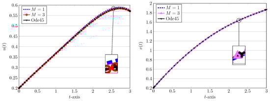
Figure 1.
Approximate solutions of (left) and (right) obtained via QLM-GMBPs based on traditional () and domain-splitting () in Example 1 with , .
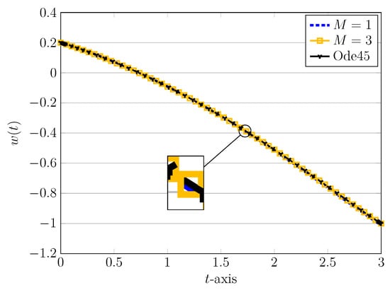
Figure 2.
Approximate solutions of obtained via QLM-GMBPs based on traditional () and domain-splitting () in Example 1 with , .
We next show that the results of direct and indirect collocation schemes i.e., the GMBPs and QLM-GMBPs matrix algorithms are coincided. Let us take and set the parameters as above. We only report the results of the direct GMBPs collocation matrix approach for as follow
It should be noted that the outcomes of QLM-GMBPs technique are very close to the above approximations and we omit them to save space. However, the achieved REFs related to both approaches are visualized in Figure 3 graphically. On the left plot, we show the REFs of direct GMBPs collocation method using while on the right picture we depict the REFs utilizing in the QLM-GMBPs matrix technique. It is clearly seen that in the direct approach we have problem with the convergence of the method if we increase P. The reason may be the fact that the used nonlinear solver fails to give us a reasonable approximation. On the other hand, we can utilize larger values of P in the QLM-GMBPs technique to reach at more accurate results. Moreover, the latter iterative method has more efficacy than the direct method. For instance, for , the required time to solve the fundamental matrix Equation (31) is about s while the elapsed time for the corresponding matrix equation via QLM-GMBPs procedure is approximately s. Consequently, in the following experiments, we usually run the latter numerical approach due to its efficacy.
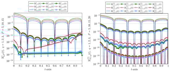
Figure 3.
The obtained REFs via GMBPs (left) and QLM-GMBPs (right) methods in Example 1 with for and different .
We further show the utility of QLM-GMBPs approach by using and a relatively large interval . The results of approximations on the first and last subibtervals and are obtained as follow
for and
for . In Figure 4 and Figure 5 we depict all approximate solutions on the domains for . The results of the ode45 are also plotted to show the validity of our approximations. By looking at these figures we find that the results of both numerical strategies are overlapped. We get a higher order accuracy if we increase the number of bases or use a lager value of subdivisions M. We next take . The 3D pictorial representation of uvw-plot as well as the 2D depiction of uv-plot are displayed in Figure 6, which show the chaotic dynamical behavior of the financial system (1). Furthermore, the similar results related to 2D representations of uw/vw-plot are shown in the next Figure 7. For validation, the numerical approximations using the ode45 are also displayed in this figure for comparison purposes. It is clear that the outcomes of both approaches are coincided.
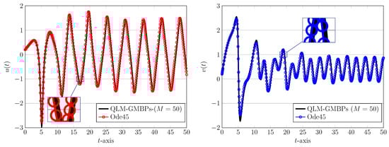
Figure 4.
Approximate solutions of (left) and (right) obtained via QLM-GMBPs based on domain-splitting () in Example 1 with , .
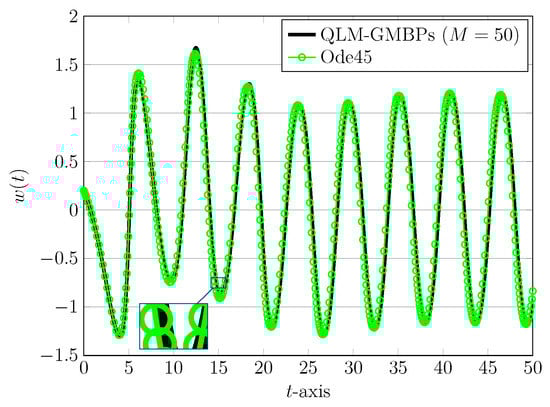
Figure 5.
Approximate solutions of obtained via QLM-GMBPs based domain-splitting () in Example 1 with , .
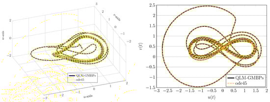
Figure 6.
3D uvw-portrait (left) and 2D uv-portrait (right) of approximate solutions obtained via QLM-GMBPs based on domain-splitting () in Example 1 with , .
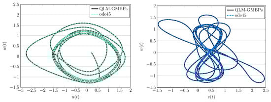
Figure 7.
2D uw-portrait (left) and 2D vw-portrait (right) of approximate solutions obtained via QLM-GMBPs based on domain-splitting () in Example 1 with , .
We now pay attention to the non-integer cases and consider . Using the domain-splitting approach along with the QLM-GMBPs strategy we plot the approximate solutions in Figure 8. We utilize the values of parameter to be both 1 and equal to . As shown in this figure, the results obtained to and are very close together. However, the REFs achieved by using are smaller in magnitude compared to those obtained by as presented in Figure 9. Note that one gets more accurate results by increasing P. Towards this end, we employ different values of P in the next experiments and report the maximum values of REFs and their associated order of convergence, i.e., for . These simulation results are tabulated in Table 1. We use , , and . The parameter is taken as . Clearly, the exponential order of convergence is visible for the results presented in Table 1. Of course, a slightly higher order of accuracy is seen for the case compared to .
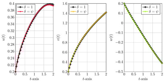
Figure 8.
Approximate solutions obtained via QLM-GMBPs based on domain-splitting () in Example 1 with , , and .
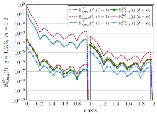
Figure 9.
The obtained REFs via QLM-GMBPs based on domain-splitting () in Example 1 with , , and .

Table 1.
The outcomes of maximum REFs error norms and the related for achieved via QLM-GMBPs in Example 1 with , , and different P.
Finally, we employ diverse values of fractional orders and visualize the numerical simulations for the three approximated solutions of system (1). We utilize , , and the parameter is equal to one. These experimental results are depicted in Figure 10 and Figure 11. We also plotted the results related to in these figures.
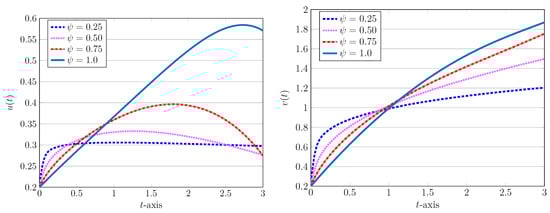
Figure 10.
Approximate solutions of (left) and (right) obtained via QLM-GMBPs based domain-splitting () in Example 1 with , , and .
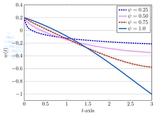
Figure 11.
Approximate solutions of obtained via QLM-GMBPs based domain-splitting () in Example 1 with , , and .
6. Conclusions
Two spectral matrix collocation methods based on (novel) domain-splitting strategy developed to handle more accurately the nonlinear fractional chaotic system arsing in financial market. The considered fractional derivative is Liouville–Caputo operator and a modified and generalized version of Bessel polynomials (GMBPs) is used in the implementation of the spectral approaches. In the first and direct collocation method, we converted the underlying model into a nonlinear algebraic system whereas in the second and efficient version of the first method, we arrived at a family of algebraic system of equations to be solve iteratively. To solve the model on a long domain, we employed the technique of domain-splitting together with aforementioned spectral schemes, which lead to a higher-order accuracy compared to traditional spectral approaches. A convergence theorem related to GMBPs established and an upper bound for the error was given. To support the theoretical findings, diverse computational experiments were conducted to show the utility of the proposed collocation approaches. The results presented through figures and tables indicate the improvement of the spectral methods based on domain-splitting strategy.
Author Contributions
Conceptualization, M.I. and H.M.S.; methodology, M.I. and H.M.S.; software, M.I.; validation, M.I. and H.M.S.; formal analysis, M.I. and H.M.S.; funding acquisition, H.M.S.; investigation, M.I. and H.M.S.; writing-original draft preparation, M.I.; writing-review and editing, M.I. and H.M.S. All authors have read and agreed to the published version of the manuscript.
Funding
This research received no external funding.
Data Availability Statement
Not Applicable.
Conflicts of Interest
The authors declare no conflict of interest.
References
- Devaney, R.L.; Keen, L. Chaos and Fractals: The Mathematics behind the Computer Graphics; American Mathematical Society: Providence, RI, USA, 1989. [Google Scholar]
- Biswas, H.R.; Hasan, M.M.; Bala, S.K. Chaos theory and its applications in our real life. Barishal Univ. J. Part 1 2018, 5, 123–140. [Google Scholar]
- Ma, Y.C.J. Study for the bifurcation topological structure and the global complicated character of a kind of non-linear finance system (I). Appl. Math. Mech. 2001, 22, 1240–1251. [Google Scholar] [CrossRef]
- Ma, Y.C.J. Study for the bifurcation topological structure and the global complicated character of a kind of non-linear finance system (II). Appl. Math. Mech. 2001, 22, 1375–1382. [Google Scholar] [CrossRef]
- Chen, W.C. Nonlinear dynamics and chaos in a fractional-order financial system. Chaos Solitons Fractals 2008, 36, 1305–1314. [Google Scholar] [CrossRef]
- Kilbas, A.A.; Srivastava, H.M.; Trujillo, J.J. Theory and Application of Fractional Differential Equations. In North-Holland Mathematics Studies; Elsevier: Amsterdam, The Netherlands, 2006; Volume 204. [Google Scholar]
- Hartle, T.T.; Lorenzo, C.F.; Qammer, H.K. Chaos in a fractional order Chua’s system. IEEE Trans CAS-I 1995, 42, 485–490. [Google Scholar] [CrossRef]
- Li, C.; Peng, G. Chaos in Chen’s system with a fractional order. Chaos Solitons Fractals 2004, 22, 443–450. [Google Scholar] [CrossRef]
- Li, C.; Chen, G. Chaos and hyperchaos in fractional order Rossler equation. Physica A 2004, 341, 55–61. [Google Scholar] [CrossRef]
- Grigorenko, I.; Grigirenko, E. Chaotic dynamics of the fractional Lorenz system. Phys. Rev. Lett. 2003, 91, 034101. [Google Scholar] [CrossRef]
- Izadi, M.; Srivastava, H.M. Fractional clique collocation technique for numerical simulations of fractional-order Brusselator chemical model. Axioms 2022, 11, 654. [Google Scholar] [CrossRef]
- Sabermahani, S.; Ordokhani, Y. Numerical solution of a fractional epidemic model via general Lagrange scaling functions with bibliometric analysis. In Mathematical Analysis of Infectious Diseases; Academic Press: Cambridge, MA, USA, 2022; pp. 305–320. [Google Scholar]
- Bidarian, M.; Saeedi, H.; Baloochshahryari, M.R. A Legendre Tau method for numerical solution of multi-order fractional mathematical model for COVID-19 disease. Comput. Methods Differ. Equ. 2023. [Google Scholar] [CrossRef]
- Owolabi, K.M.; Atangana, A.; Gómez-Aguilar, J.F. Fractional Adams-Bashforth scheme with the Liouville-Caputo derivative and application to chaotic systems. Discret. Contin. Dyn. Syst. S 2021, 14, 2455. [Google Scholar] [CrossRef]
- Alquran, M.; Alsukhour, M.; Ali, M.; Jaradat, I. Combination of Laplace transform and residual power series techniques to solve autonomous n-dimensional fractional nonlinear systems. Nonlinear Eng. 2021, 10, 282–292. [Google Scholar] [CrossRef]
- Adel, M.; Khader, M.M.; Ahmad, H.; Assiri, T.A. Approximate analytical solutions for the blood ethanol concentration system and predator-prey equations by using variational iteration method. AIMS Math. 2023, 8, 19083–19096. [Google Scholar] [CrossRef]
- Sunthrayuth, P.; Dutt, H.M.; Ghani, F.; Arefin, M.A. The analysis of fractional-order system delay differential equations using a numerical Method. Complexity 2022, 2022, 3570667. [Google Scholar] [CrossRef]
- Ma, S.; Xu, Y.; Yue, W. Numerical solutions of a variable-order fractional financial system. J. Appl. Math. 2012, 2012, 417942. [Google Scholar] [CrossRef]
- Moutsinga, C.R.B.; Pindza, E.; Mare, E. A robust spectral integral method for solving chaotic finance systems. Alex. Eng. J. 2020, 59, 601–611. [Google Scholar] [CrossRef]
- Farman, M.; Akgül, A.; Saleem, M.U.; Imtiaz, S.; Ahmad, A. Dynamical behaviour of fractional-order finance system. Pramana 2020, 164, 94. [Google Scholar] [CrossRef]
- Shabani, A.; Sheikhani, A.R.; Aminikhah, H. Robust Control for variable order time fractional financial system. Dyn. Syst. Appl. 2020, 29, 111–122. [Google Scholar] [CrossRef]
- Junswang, P.; Sabir, Z.; Raja, M.A.Z.; Adel, W.; Botmart, T.; Weera, W. Intelligent networks for chaotic fractional-order nonlinear financial model. Comput. Mater. Contin. 2022, 72, 5015–5030. [Google Scholar] [CrossRef]
- Ahmad, I.; Ouannas, A.; Shafiq, M.; Pham, V.T.; Baleanu, D. Finite-time stabilization of a perturbed chaotic finance model. J. Adv. Res. 2022, 32, 1–14. [Google Scholar] [CrossRef]
- Gao, W.; Veeresha, P.; Baskonus, H.M. Dynamical analysis fractional-order financial system using efficient numerical methods. Appl. Math. Sci. Eng. 2023, 31, 2155152. [Google Scholar] [CrossRef]
- Xu, C.J.; Liu, Z.X.; Liao, M.X.; Yao, L.Y. Theoretical analysis and computer simulations of a fractional order bank data model incorporating two unequal time delays. Expert Syst. Appl. 2022, 199, 116859. [Google Scholar] [CrossRef]
- Srivastava, H.M.; Raghavan, D.; Nagarajan, S. A comparative study of the stability of some fractional-order cobweb economic models. Rev. Real Acad. Cienc. Exactas Fís. Natur. Ser. A Mat. (RACSAM) 2022, 116, 98. [Google Scholar] [CrossRef]
- Edeki, S.O.; Okoli, D.C.; Ahmad, H.; Wong, W.K. Approximate series solutions of a one-factor term structure model for bond pricing. Ann. Financ. Econ. 2021, 16, 1–22. [Google Scholar] [CrossRef]
- Odibat, Z.M.; Shawagfeh, N.T. Generalized Taylor’s formula. Appl. Math. Comput. 2007, 186, 286–293. [Google Scholar] [CrossRef]
- Van Rossum, H. Totally positive polynomials. Proc. Kon. Nederl. Akud. Wetensch. Ser. A 1965, 68; Zndag. Math. 1965, 27, 305–315. [Google Scholar] [CrossRef]
- Krall, H.L.; Frink, O. A new class of orthogonal polynomials: The Bessel polynomials. Trans. Am. Math. Soc. 1949, 65, 100–115. [Google Scholar] [CrossRef]
- Izadi, M.; Cattani, C. Generalized Bessel polynomial for multi-order fractional differential equations. Symmetry 2020, 12, 1260. [Google Scholar] [CrossRef]
- Ahmed, S.S.; MohammedFaeq, S.J. Bessel collocation method for solving Fredholm-Volterra integro-fractional differential equations of multi-high order in the Caputo sense. Symmetry 2021, 13, 2354. [Google Scholar] [CrossRef]
- Izadi, M. Numerical approximation of Hunter-Saxton equation by an efficient accurate approach on long time domains. U.P.B. Sci. Bull. Ser. A 2021, 83, 291–300. [Google Scholar]
- Izadi, M.; Yüzbası, S.; Noeiaghdam, S. Approximating solutions of non-linear Troesch’s problem via an efficient quasi-linearization Bessel approach. Mathematics 2021, 9, 1841. [Google Scholar] [CrossRef]
- Yüzbası, S.; Izadi, M. Bessel-quasilinearization technique to solve the fractional-order HIV-1 infection of CD4+ T-cells considering the impact of antiviral drug treatment. Appl. Math. Comput. 2022, 431, 127319. [Google Scholar] [CrossRef]
- Izadi, M.; Yüzbası, S.; Cattani, C. Approximating solutions to fractional-order Bagley-Torvik equation via generalized Bessel polynomial on large domains. Ric. Mat. 2023, 72, 235–261. [Google Scholar] [CrossRef]
- Srivastava, H.M. An introductory overview of Bessel polynomials, the generalized Bessel polynomials and the q-Bessel polynomials. Symmetry 2023, 15, 822. [Google Scholar] [CrossRef]
- Izadi, M.; Yüzbası, S.; Adel, W. A new Chelyshkov matrix method to solve linear and nonlinear fractional delay differential equations with error analysis. Math. Sci. 2022. [Google Scholar] [CrossRef]
- Aznam, S.M.; Ghani, N.A.; Chowdhury, M.S. A numerical solution for nonlinear heat transfer of fin problems using the Haar wavelet quasilinearization method. Results Phys. 2019, 14, 102393. [Google Scholar] [CrossRef]
- Izadi, M. A combined approximation method for nonlinear foam drainage equation. Sci. Iran. 2022, 29, 70–78. [Google Scholar] [CrossRef]
- Ahmed, S.; Jahan, S.; Nisar, K.S. Hybrid Fibonacci wavelet method to solve fractional-order logistic growth model. Math. Meth. Appl. Sci. 2023. [Google Scholar] [CrossRef]


Disclaimer/Publisher’s Note: The statements, opinions and data contained in all publications are solely those of the individual author(s) and contributor(s) and not of MDPI and/or the editor(s). MDPI and/or the editor(s) disclaim responsibility for any injury to people or property resulting from any ideas, methods, instructions or products referred to in the content. |
© 2023 by the authors. Licensee MDPI, Basel, Switzerland. This article is an open access article distributed under the terms and conditions of the Creative Commons Attribution (CC BY) license (https://creativecommons.org/licenses/by/4.0/).