Abstract
Random vibration analysis is a mathematical tool that offers great advantages in predicting the mechanical response of structural systems subjected to external dynamic loads whose nature is intrinsically stochastic, as in cases of sea waves, wind pressure, and vibrations due to road asperity. Using random vibration analysis is possible, when the input is properly modeled as a stochastic process, to derive pieces of information about the structural response with a high quality (if compared with other tools), especially in terms of reliability prevision. Moreover, the random vibration approach is quite complex in cases of non-linearity cases, as well as for non-stationary inputs, as in cases of seismic events. For non-stationary inputs, the assessment of second-order spectral moments requires resolving the Lyapunov matrix differential equation. In this research, a numerical procedure is proposed, providing an expression of response in the state-space that, to our best knowledge, has not yet been presented in the literature, by using a formal justification in accordance with earthquake input modeled as a modulated white noise with evolutive parameters. The computational efforts are reduced by considering the symmetry feature of the covariance matrix. The adopted approach is applied to analyze a multi-story building, aiming to determine the reliability related to the maximum inter-story displacement surpassing a specified acceptable threshold. The building is presumed to experience seismic input characterized by a non-stationary process in both amplitude and frequency, utilizing a general Kanai–Tajimi earthquake input stationary model. The adopted case study is modeled in the form of a multi-degree-of-freedom plane shear frame system.
1. Introduction
Taking into account how structures behave in a random vibration setting is a prevalent method used to assess actual response scenarios [1]. This applies to various contexts, e.g., aircraft, vibrating machinery, and buildings subjected to marine or wind vibrations. These engineering scenarios involve examining how structures respond to dynamic and nondeterministic actions, and random dynamic analysis proves to be the most effective mathematical tool for this purpose [2]. This decision arises from the inherent randomness in inputs, a well-documented aspect in the field of random vibration theory (as evidenced by [3,4,5,6]). Approaching the problem using these methodologies enables acquiring relevant and reliable information about the structural response, typically unattainable through deterministic methods. The strength of the random vibration approach lies in its high-quality information, including the quantification of structural integrity, which is significant in probabilistic safety assessments. Failure is generally described as the initial moment when a structural crisis begins, tying it to the first instance where one or more measurements of structural response exceed a safe range. This usually involves assessing structural response indicators like displacements, stresses, buckling loads, or natural frequencies.
The random vibration problem for linear mechanical systems subject to Gaussian processes input is posed in stationary environmental conditions as the solution of the so-called Lyapunov matrix equation [7,8] to obtain the response covariance that defines completely the statistics of the system. Challenges in solving the Lyapunov equation have constrained the size of the meshes that could be employed. The Lyapunov equation (i.e., Lyapunov matrix equation, , A system matrix, R covariance matrix, and B input matrix, see Section 2) is typically achieved using algorithms like Bartels–Steward or Hessenberg–Schur. These methods require the Schur factorization of system matrix A. Various software tools for scientific computing, such as Matlab and Python, employ adapted versions of these algorithms, delivering satisfactory results for small dense matrices A and B. This involves O floating-point operations and O memory [9]. Approaches designed for large system dimensions have been developed, for instance, the Krylov subspace methods [9,10,11] or the matrix sign function decomposition with Newton’s iterative method.
In non-stationary cases, under the same assumptions (linear system and Gaussian input) the time covariance approach is more complex as the Lyapunov matrix covariance becomes a differential one (i.e., Lyapunov differential matrix equation, , see Section 3) whose numerical solution is sometimes more complex, and there are not standard tools to be implemented, differently from the stationary case.
The main objective of this research is to introduce a numerical technique for evaluating response covariance in the time domain for linear structures subjected to non-stationary stochastic loads. This method is tailored for a generic scenario where the input involves a non-stationary modulated filtered white noise process, capable of simulating various real physical loads like earthquakes [12,13,14,15].
To achieve a versatile non-stationary approach applicable across different contexts, the structural response is assessed using a covariance approach, as understanding the evolving covariance matrix in the space state is crucial for evaluating reliability, particularly in terms of initial failure events.
To address this, a time-step integration algorithm is proposed, employing the Euler implicit method to solve the differential Lyapunov matrix equation. The outcome is a sequential algorithm that requires the numerical solution of a stationary Lyapunov matrix equation at each time step, a task achievable through standard numerical tools. This method is implemented to reduce computational expenses and has been specifically applied to a multi-story building represented by a shear frame structure, examining dynamic responses under seismic base motions and assessing the reliability concerning initial threshold crossings.
2. Linear Elastic MDoF Subject to Non-Stationary Random Vibration
Many instances of real-life structural issues revolve around configurations that match a linear viscoelastic system of lumped masses. These systems face either steady or fluctuating forces. This study considers both scenarios to evaluate how structural responses vary statistically, employing the covariance approach [13,14].
This method presents notable benefits, especially in dynamic conditions, where inputs are simulated as white noises. These can be filtered to better match real dynamic occurrences. By solving the equations of the dynamic equilibrium system, this technique gauges the structural response of a deterministic second-order linear mechanical system composed of lumped masses when subjected to probabilistic dynamic input.
where , and are the structural displacement, velocity, and acceleration process vectors. , and are the mass, viscous, and stiffness symmetric matrices. While the mass matrix is always positive definite, the damping and stiffness matrices are positive semi-definite. The vector
accumulates n stochastic excitations applied to the structure, while Gs represents an m x n matrix linking the excitation components of the forcing vector to the structural degrees of freedom. When the elements of the system excitations vector are stationary white noises, the first- and second-order statistical moments remain unchanged over time.
Moreover, if are Gaussian excitations, then the responses and their time derivatives constitute a Markov vector in the dimension phase state.
The matrix, related to a vector satisfying the shot noise properties (usually denoted as a shot noise vector), has diagonal elements equal to the autocovariance intensity of each force and extra-diagonal elements representing the level of correlation between two generic different forces, so that can vary from if and are completely correlated, to zero, if and are completely un-correlated.
Then, in the case of complete un-correlated forcing loads, the matrix is replaced by the simpler diagonal matrix of components, where the elements are the input power spectral density of each entry.
A commonly used method involves expressing a non-stationary input through an intensity modulation of a stationary process, often referred to as uniform modulation. This method assumes that the intensity of the process alters over time according to a deterministic function , while the spectral contents remain constant. Consequently, in the case of time modulation, a stationary forcing process vector is substituted by the following non-stationary vector:
with the stochastic characterization
and, in case of un-correlated excitations, the covariance matrix is diagonal
Pre Filters Technique
In time-domain stochastic analysis, two primary methods are typically employed. The first, applicable when the input’s autocorrelation function is known, has been previously outlined. The second involves modeling input processes by solving differential equations using filter techniques, where the input is a white noise process—referred to as the pre-filter technique.
The first method is advantageous when the input closely aligns with a shot noise process, providing accurate representation. However, this representation is limited as many real-world phenomena exhibit noticeable frequency modulation, making it suitable only in specific cases.
The second approach is more versatile and capable of representing phenomena with varying frequency contents, even those changing over time. This flexibility is crucial for accurately describing phenomena that could lead to resonant effects in structures. Additionally, this method retains the advantages associated with shot noise inputs, making it the preferred choice for many real structural issues.
In particular, using the pre-filter approach, the filter response is described by the filter space state vector, the solution of the set of differential equations
that generally could have a time-dependent form, when not only the frequency but also the amplitude of loads has an intrinsic evolutive nature. is a vector of white noise processes (stationary or non-stationary), is a matrix that couples the excitation components of the forcing vector to the filter degree of freedom, and finally, is the X. filter system matrix, whose generic form is
Then, adopting the pre-filter technique, the motion differential equations are written in the space state as
where
is the structural system matrix
is a time-dependent matrix
is the structural space vector. Equations for the space state structure can be summarized as
where
is a new global space state vector (structure plus filter) and
The structural matrix and response vectors are contingent on the design parameter vector , which encompasses elements such as structural stiffness, damping, masses, and various mechanical parameters like cross-sections, Young’s modulus, and boundary conditions, among others. Filter parameters and input intensity are also included within this set of design parameters. Consequently, the system matrix and equations, comprising both the space state structure and filter equation, can be explicitly reconfigured as a function of this design parameter vector:
3. Space State Covariance Evaluation
In case of zero initial conditions, the solution of (space state structure + filter equation) has the following general expression:
where the matrix (see for example [3]) is usually called transition matrix. The mean space state vector could be determined by the differential vectorial equation:
The covariance matrix is as follows:
This second-order statistical moments matrix, due to its symmetry, is described by independent elements and can be evaluated by the well-known Lyapunov differential matrix equation
where
and where can be written as
and
It must be noticed that Equation (25), which is valid for the non-stationary case, in a stationary environmental situation, is simplified in the following equation that contains no more time dependency:
A serious simplification takes place when the forcing vector is a white noise process as defined in (Rww stationary) or (Rww non-stationary). In these cases, the matrix is equal to
where both integrals above are equal due to the Dirac function properties. Finally, B can be written as follows:
where the MXM submatrix is diagonal with the elements
Meanwhile, for some applications, covariance information about structural acceleration is needed so that the matrix
must be determined, and it is easily obtainable by the relation
where
4. Time Integration BF Procedure for and
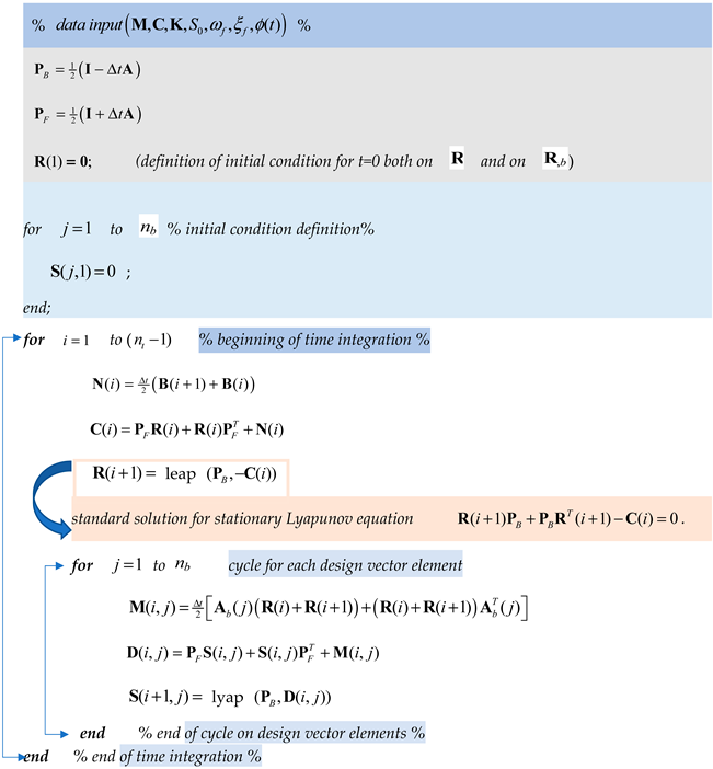
Even if many numerical standard codes exist for the stationary Lyapunov equation (the Lyapunov equation in stationary conditions is where A and B are the input matrices and X is the unknown one), there are limited examples for addressing the non-stationary Lyapunov equation, and so a simple numeric implicit integration method is proposed. In this context, a straightforward numerical implicit integration method is suggested. Specifically, the modified Euler method is used, in which the period is divided in equals time steps d in each sub-period and a linear variation in the time derivative covariance matrix is assumed. Under this assumption, we have the (standard implicit Euler method):
where the symbol denotes the generic quantity evaluated at time . By using the matrix equations evaluated at times and , we obtain the following algebraic matrix equations of the Lyapunov type
that are solved in sequence for each time value, starting from the initial time value and the initial covariance matrix value.
In this way, the m unknown matrices are determined. By assuming a constant or time variable (depending on the filter parameters variation), the matrices are
and we discern that a more compact form of (Rnum1) is
that could be solved at each step via a standard stationary Lyapunov equation solver, for example, the leap in the standard Matlab toolbox, in the form
where .
Covariance could be integrated as proposed in the following integration scheme (Algorithm 1), where is the number of time integration steps, is the total analysis time, the number of design parameters, and, for the sake of simplicity in notation, :
| Algorithm 1: Integration scheme |
 |
5. Numerical Example
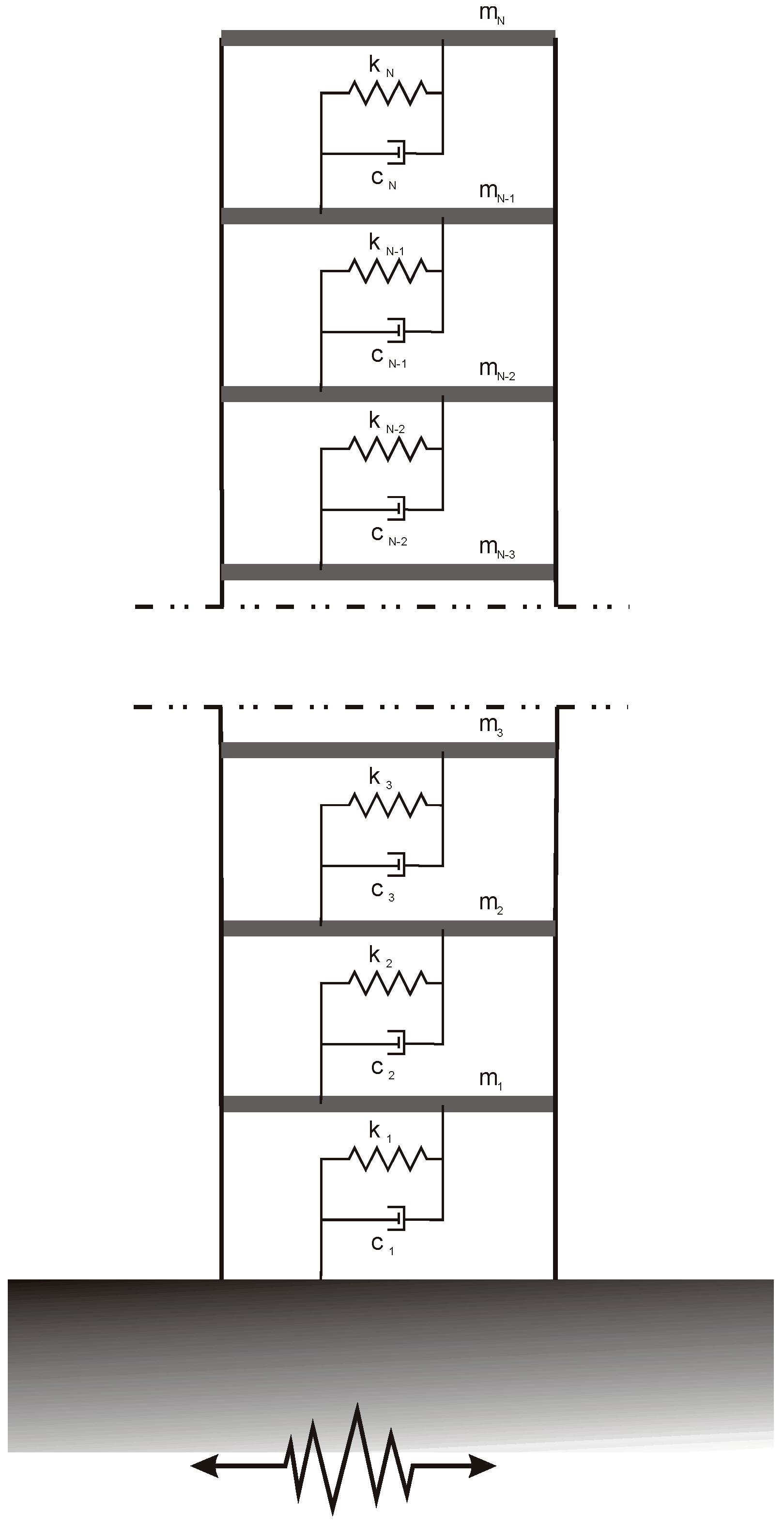
The method proposed is used to analyze a multi-story building under earthquake forces. To maintain a balance between simplicity and generality, a shear-type plane frame structure is chosen as the model (as shown in Figure 1). This choice is reasonable because, in many buildings, the floor slabs possess very high in-plane stiffness, allowing them to be treated as rigid diaphragms. This simplification significantly enhances analysis efficiency without substantially compromising the accuracy of response assessment to ground forces.
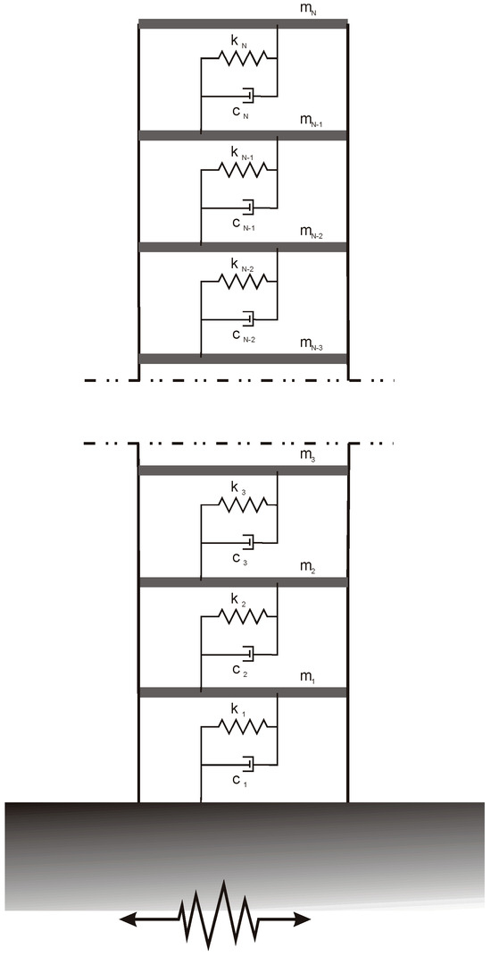
Figure 1.
Mechanical scheme of analyzed plane frame shear type.
Moreover, to further enhance computational efficiency, the matrix condensation technique is employed. The primary assumption in modeling the building’s mechanics is linearity, which remains valid considering the limitations on horizontal displacements necessary for operational service levels. This assumption holds when the maximum inter-story drift approaches or reaches the elastic limit of structural displacements, typical in full operational design demands.
For the sensitivity analysis, the design vector comprises the masses, stiffness, and damping of each floor. This comprehensive vector allows for the evaluation of how variations in these parameters impact the final structural reliability.
where .
5.1. Equations of Motion
To capture the essential seismic characteristics involving spectral and time modulation, a non-stationary modulated Kanai–Tajimi process is utilized to model stochastic ground motion. This process characterizes the base acceleration acting at the structure’s base as follows:
where is the response of the Kanai–Tajimi filter, with a frequency and damping coefficient , and is the white noise, whose constant bilateral power spectral density (PDS) function is . This last parameter is related to the peak ground acceleration (PGA) by means of relation [16]
The non-stationary nature is introduced through the deterministic temporal modulation function , regulating the intensity variations while preserving the earthquake’s frequency characteristics. In this scenario, the specific modulation functions proposed by Jennings [17] are adopted:
The motion equations for the complete structural system are then as follows:
where the drag vector is = , , , and are, respectively, mass, viscosity, and stiffness principal structure matrices, whose general expression are reported in Appendix A with reference to the rigid floor assumption. The three vectors , and are ground relative acceleration, velocity, and displacement vectors. In the case of the analyzed structure, the mass matrix is diagonal and the two viscous and stiffens matrices are tri-diagonal once. The mechanical filter parameters, the damping ratio and frequency, are and , and the base excitation is then equal to .
Introducing the state vector , the motion equation system (motion Equation (1)) can be rewritten as
where the two matrices and , with the vector , are defined for this specific problem and shown in Appendix B.
The degree of freedom -order differential system (second-order moment equals complete) can be replaced with a DoF -order differential equation in the space state as follows:
where the space vector is and the system matrix (2N X. 2N) and the forcing vector .
5.2. Reliability Evaluation
With reference to the proposed problem, it is required to evaluate the probability that each story drift of the floor exceeds the thresholds, at least once in a given earthquake duration. Then, for each level, this failure event is associated with the condition For each level , the reliability vector element is defined as where, under the Poisson hypothesis for threshold crossing (that is an acceptable hypothesis for rare events as in [18]), we obtain
and the final global structural reliability is then
Although exact analytical solutions for this are generally unavailable, it is known that the equation (approximate upper-bound global reliability) provides an approximate, upper-bound estimate, as stated above, and can be used for design and pre-design purposes from a practical viewpoint, as in this study. In order to evaluate the reliability vector (adopting the Poisson approach) related to the inter-floor relative displacement threshold crossing, one needs to introduce the inter-story drift vector with the associated covariance matrix (see Appendix C).
The reliability vector previously defined can be evaluated as the collection of
where is a function of , and , accordingly, and are, respectively, the and the diagonal elements of and , with being the barrier.
The equation represents the probability that the inter-story displacement will cross the maximum acceptable value during the time interval . All the barriers can be collected in the barrier vector. Its elements are assumed constant and equal to 3.0 cm for each floor, that is, there is a lateral drift equal to 1.0% in the case of inter-story height of 3 m.
5.3. System Parameters
The chosen building configuration consists of three stories, each with a uniform mass equal to x for each level. Lateral stiffness to the first floor is present, and it is assumed that a linear reduction decreases its value to the at the top floor ( and ). Finally, damping is evaluated by setting ( ).
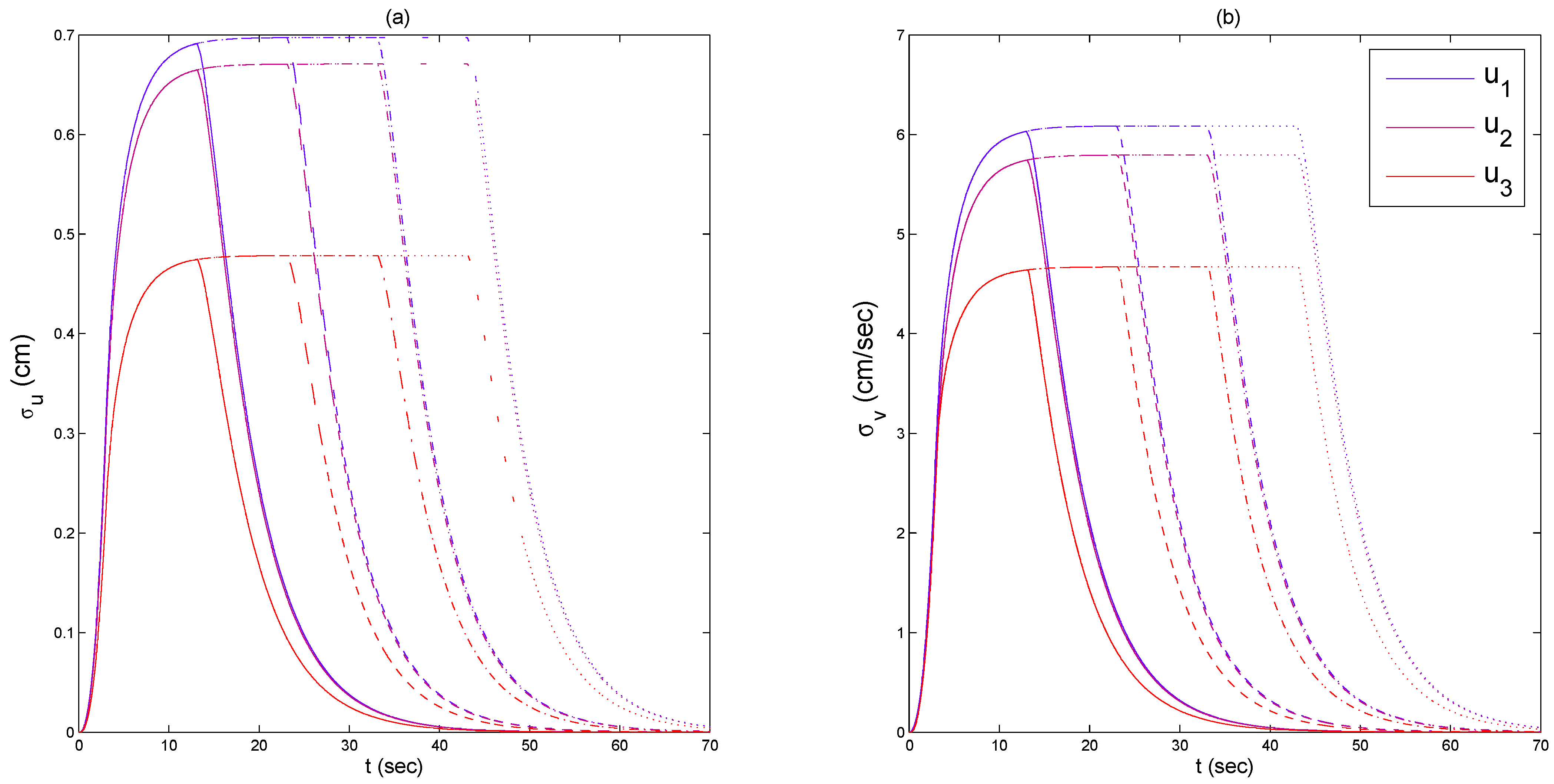
The seismic characterization is based on a peak ground acceleration (PGA) of 0.45 (g), and four distinct total durations (10, 20, 30, and 40 s) are employed. Figure 2 displays the structural inter-story covariances, measured in terms of displacement (a) and velocity (b). It is noteworthy that for durations exceeding this, structural responses attain a stationary level. Moreover, for this particular structural configuration, the covariance response of the first level is greater than the other two, even though the third is approximately half, while the second is only slightly smaller.
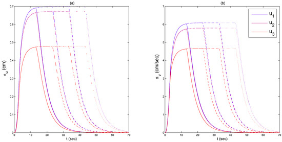
Figure 2.
Inter-story displacements (a) and velocities (b) covariance response of a 3DoF system subject to modulated filtered white noise with different time durations. Continuous lines are for t_{d} = 10 (s), dashed lines are for t_{d} = 20 (s), dash–dot lines are for t_{d} = 30 (s), and finally, dotted lines are for t_{d} = 40 (s). Blue lines represent the inter-story drift response on the first floor, magenta lines on the second floor, and red lines refer to the third floor.
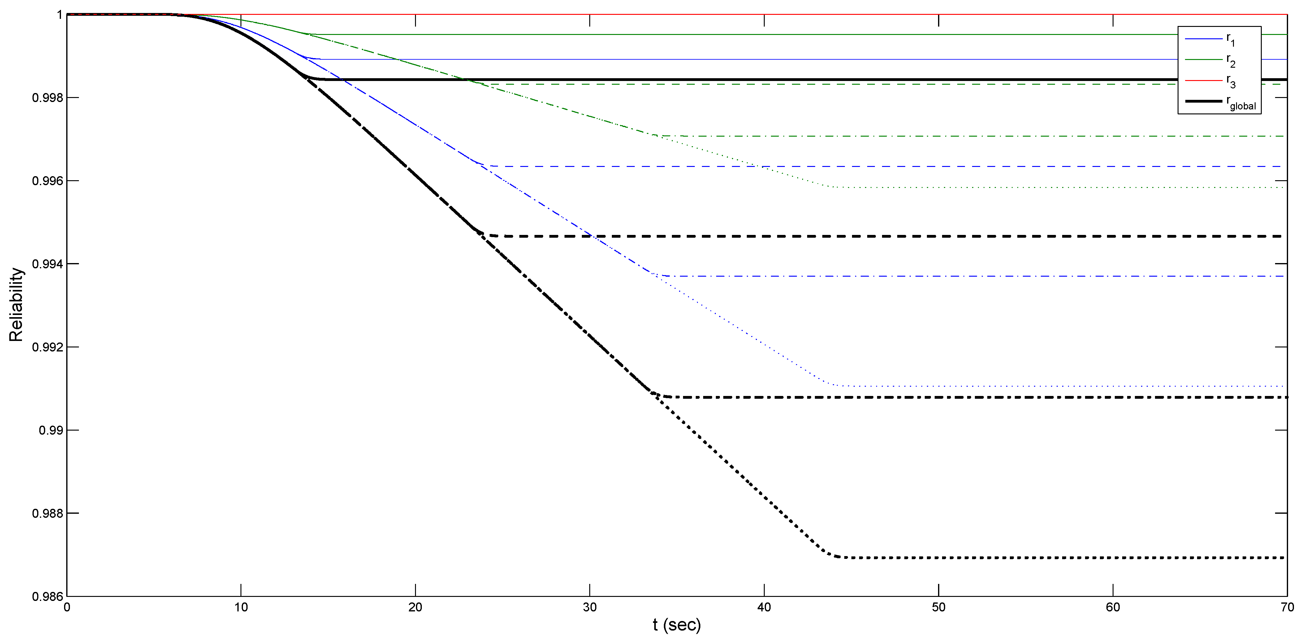
Figure 3 illustrates the structural safeties assessed at each lateral inter-story drift threshold for failure, along with the overall reliability calculated as an approximate upper-bound global reliability. It is important to observe that the probability of failure is highest for the first inter-story drift threshold, followed by a slightly lower probability for the second one, and finally, the third threshold has a considerably negligible probability of failure (i.e., ).
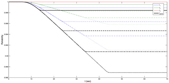
Figure 3.
System reliability of a 3DoF system, evaluated as the probability of maximum inter-story drift exceeds a given threshold of 3 (cm). Results are obtained for different values of t_{d}: continuous lines are for t_{d} = 10 (s), dashed lines are for t_{d} = 20 (s), dash–dot lines are for t_{d} = 30 (s), and finally, dotted lines are for t_{d} = 40 (s). Blue lines are for first-level reliability, magenta lines are for second-level reliability, and red lines are for third-level reliability. Black slight lines are for global system reliability.
6. Conclusions
A numerical time integration algorithm is proposed to deal with non-stationary random vibration problems utilizing a covariance approach. The algorithm is developed to solve the differential matrix equations that govern the evolution of the stochastic response of structures subjected to random inputs. To create a versatile non-stationary approach applicable in various contexts, the structural response is assessed through a covariance approach. The reliability concerning first-crossing failure events is then derived based on the knowledge of the evolving covariance matrix in the space state. The algorithm is proposed for a generic Gaussian input of filtered non-stationary processes, representing diverse real-world physical loads. To solve this problem, the time integration algorithm involves differentiating the Lyapunov equation using an adapted Euler implicit scheme, which can be easily implemented using standard tools in various programming codes. Finally, the proposed algorithm is applied to analyze the dynamic responses of a multistory building, idealized as a shear frame structure.
Author Contributions
Conceptualization, R.C. and G.C.M.; Methodology, M.D., R.C. and G.C.M.; Validation, R.C. and G.C.M.; Formal analysis, M.D., R.C. and G.C.M.; Investigation, G.C.M.; Writing—original draft, M.D., R.C. and G.C.M.; Writing—review & editing, M.D., R.C., S.L.L., M.M. and G.C.M.; Visualization, L.S.; Supervision, G.C.M. All authors have read and agreed to the published version of the manuscript.
Funding
The research leading to these results has received funding from the European Research Council under the grant agreement ID: 101007595 of the project ADDOPTML, MSCA RISE 2020 Marie Skodowska Curie Research and Innovation Staff Exchange (RISE).
Conflicts of Interest
The authors declare no conflict of interest.
Appendix A
Matrices, and are, for a shear-type frame, respectively diagonal and tri-diagonals:
Appendix B
Matrices and are
where and are filter characteristics and the forcing vector is .
Appendix C
The covariance matrix is defined in the linear space of stochastic processes as a linear equation related to the inter-story drift and displacement vectors, holds where the transform matrix is a bi-diagonal one, and is independent of the design vector:
The covariance matrix is then related to through the following connection:
References
- Liu, J.; Wang, L. Hybrid Reliability-Based Sequential Optimization for PID Vibratory Controller Design Considering Interval and Fuzzy Mixed Uncertainties. Appl. Math. Model. 2023, 122, 796–823. [Google Scholar] [CrossRef]
- Huang, H.; Li, Y.; Li, W. Dynamic reliability analysis of stochastic structures under non-stationary random excitations based on an explicit time-domain method. Struct. Saf. 2023, 101, 102313. [Google Scholar] [CrossRef]
- Soong, T.T.; Grigoriu, M. Random Vibration of Mechanical and Structural Systems; Prentice Hall: Hoboken, NJ, USA, 1993. [Google Scholar]
- Lin, Y.K. Probabilistic Theory of Structural Dynamics; Wax, N., Ed.; Stochastic Processes; Krieger Publishing, Co., Inc.: Huntington, NY, USA, 1967. [Google Scholar]
- Lutes, L.D.; Sarkani, S. Stochastic Analysis of Structural and Mechanical Vibration; Prentice-Hall Inc.: Hoboken, NJ, USA, 1997. [Google Scholar]
- Nigam, N.C.; Narayanan, S. Application of Random Vibration; Narosa Publishing House: Delhi, India, 1994. [Google Scholar]
- Gomez, F.; Spencer, B.F., Jr.; Carrion, J. Topology optimization of buildings subjected to stochastic base excitation. Eng. Struct. 2020, 23, 111111. [Google Scholar] [CrossRef]
- Spencer, B.F.; Gomez, F.; Xu, J. Topology Optimization for Stochastically Excited Structures; ISSRI: Uttar Pradesh, India, 2016. [Google Scholar]
- Kressner, D. Memory-efficient Krylov subspace techniques for solving large-scale Lyapunov equations. In Proceedings of the 2008 IEEE International Conference on Computer-Aided Control Systems, San Antonio, TX, USA, 3–5 September 2008; IEEE: Piscataway, NJ, USA, 2008; pp. 613–618. [Google Scholar]
- Saad, Y. Numerical Solution of Large Lyapunov Equations; Signal Process Scattering Oper Theory Numer Methods, Proc MTNS-89; Birkhauser: Basel, Switzerland, 1989; Volume 3, pp. 503–511. [Google Scholar]
- Jbilou, K.; Riquet, A. Projection methods for large Lyapunov matrix equations. Linear Algebra Appl. 2006, 415, 344–358. [Google Scholar] [CrossRef]
- Muscolino, G.; Genovese, F.; Biondi, G.; Cascone, E. Generation of fully non-stationary random processes consistent with target seismic accelerograms. Soil Dyn. Earthq. Eng. 2021, 141, 106467. [Google Scholar] [CrossRef]
- Marano, G.C.; Acciani, G.; Fiore, A.; Abrescia, A. Integration algorithm for covariance Nonstationary dynamic analysis of SDOF systems using equivalent stochastic linearization. Int. J. Struct. Stab. Dyn. 2015, 15, 1450044. [Google Scholar] [CrossRef]
- Greco, R.; Marano, G.C.; Fiore, A.; Vanzi, I. Nonstationary First Threshold Crossing Reliability for Linear System Excited by Modulated Gaussian Process. Shock. Vib. 2018, 2018, 3685091. [Google Scholar] [CrossRef]
- Sgobba, S.; Stafford, P.J.; Marano, G.C.; Guaragnella, C. An evolutionary stochastic ground-motion model defined by a seismological scenario and local site conditions. Soil Dyn. Earthq. Eng. 2011, 31, 1465–1479. [Google Scholar] [CrossRef]
- Crandall, S.H.; Mark, W.D. Random Vibration in Mechanical Systems; Academic Press: Cambridge, MA, USA, 1963. [Google Scholar]
- Jennings, P.C. Periodic response of a general yielding structure. J. Eng. Mech. Div. 1964, 90, 131–166. [Google Scholar] [CrossRef]
- Vanmarcke, E.H. On the Distribution of the First-Passage Time for Normal Stationary Random Processes. ASME J. Appl. Mech. March 1975, 42, 215–220. [Google Scholar] [CrossRef]
Disclaimer/Publisher’s Note: The statements, opinions and data contained in all publications are solely those of the individual author(s) and contributor(s) and not of MDPI and/or the editor(s). MDPI and/or the editor(s) disclaim responsibility for any injury to people or property resulting from any ideas, methods, instructions or products referred to in the content. |
© 2024 by the authors. Licensee MDPI, Basel, Switzerland. This article is an open access article distributed under the terms and conditions of the Creative Commons Attribution (CC BY) license (https://creativecommons.org/licenses/by/4.0/).