Article

Taylor Polynomials in a High Arithmetic Precision as Universal Approximators

1
Computation-Based Science and Technology Research Center, The Cyprus Institute, 20 Konstantinou Kavafi Str., 2121 Nicosia, Cyprus
2
Department of Information Technology & AI Lab, American College of Greece, Deree. 6 Gravias Str., Aghia Paraskevi, 15342 Athens, Greece
Computation 2024, 12(3), 53; https://doi.org/10.3390/computation12030053
Submission received: 14 January 2024 / Revised: 12 February 2024 / Accepted: 22 February 2024 / Published: 7 March 2024
(This article belongs to the Special Issue Computational Methods in Structural Engineering)

Abstract

:
Function approximation is a fundamental process in a variety of problems in computational mechanics, structural engineering, as well as other domains that require the precise approximation of a phenomenon with an analytic function. This work demonstrates a unified approach to these techniques, utilizing partial sums of the Taylor series in a high arithmetic precision. In particular, the proposed approach is capable of interpolation, extrapolation, numerical differentiation, numerical integration, solution of ordinary and partial differential equations, and system identification. The method employs Taylor polynomials and hundreds of digits in the computations to obtain precise results. Interestingly, some well-known problems are found to arise in the calculation accuracy and not methodological inefficiencies, as would be expected. In particular, the approximation errors are precisely predictable, the Runge phenomenon is eliminated, and the extrapolation extent may a priory be anticipated. The attained polynomials offer a precise representation of the unknown system as well as its radius of convergence, which provides a rigorous estimation of the prediction ability. The approximation errors are comprehensively analyzed for a variety of calculation digits and test problems and can be reproduced by the provided computer code.

1. Introduction

The utilization of a high arithmetic precision (HAP) for the modeling of an unknown function exhibited a remarkable extrapolation ability in [1], with extrapolation spans 1000% higher than the existing methods in the literature. The basis of this method was the approximation of an unknown analytic function with a high arithmetic precision. This is an essential problem in a variety of numerical methods. Standard programming languages are limited to 16–64 floating point digits, and researchers have been taking into account a high arithmetic precision for the various computations regarding the numerical integration [2], interpolation [3], and solution of Partial Differential Equations (PDEs) [4].
Recent research works highlight the importance of a HAP in computations. In [5], the Clarinet framework is proposed to replace floating point arithmetic in various linear algebra and computer vision calculations. The effect of round-off errors when utilizing a standard accuracy for reduction algorithms is highlighted in [6], and a high-precision “RingAllreduce” algorithm was proposed. A high-precision ray-tracing algorithm is presented in [7], reducing round-off errors in the numerical examples. A high arithmetic precision is also significant in the design of Field Programmable Gate Arrays (FPGAs), and a new representation to tackle programming challenges is proposed in [8]. The GNU Multiple Precision Arithmetic Library (GMP) [9] is a widely used library in many computer languages, like C++, Python, and Julia, and a framework to enable its usage by Java was recently developed [10].
Nevertheless, standard techniques exist for performing interpolation with Taylor polynomials [11,12], as well as the solution of differential equations [13,14,15]. However, certain problems occur when applying these methods for scientific computing tasks, such as the well-known Runge phenomenon [16,17], which remains a major complication [18,19,20]. Taylor series arise in the foundations of differential calculus [21] by associating the behavior of a function around a point x 0 with its derivatives at that particular point.
Accordingly, Taylor series are capable of approximating any analytic function in theory. However, in the practice of computing, they often fail, and researchers use other approximators than Taylor polynomials, such as radial basis functions, Lagrange polynomials, Chebyshev polynomials, artificial neural networks, etc., to avoid numerical instabilities. A variety of numerical methods have been developed for such operations, as researchers have been observing that Taylor polynomials do not offer stable calculations. Utilizing a high arithmetic precision, we demonstrate that such need, which arose to address the computational inaccuracies, does not exist. Taking into account the high extrapolation spans attained in [1] and obtained with integrated radial basis functions [22,23] and some hundreds or even thousands of digits for the calculations, we apply a high arithmetic precision utilizing the “BigFloat” structure of Julia language [24], using the GMP [9] library to truncate the Taylor series, known as Taylor polynomials or partial sums.
The purpose of this work is to present a unified approach to interpolation, extrapolation, numerical differentiation, solution of partial differential equations, system identification, and numerical integration for problems which comprise given data of an unknown analytic function or the source for PDEs. The paper is organized as follows: the formulation of our approach is presented in Section 2; some basic operations and results for 1-dimensional interpolation, extrapolation, numerical differentiation, numerical integration, and solutions of ordinary differential equations are presented in Section 3; the results of multidimensional function approximation, solution of partial differential equations, and system identification are presented in Section 4; and the conclusions follow in Section 5.
Taylor polynomials provide a fundamental means to approximate complex functions and understand their behavior, such as rate of change, curvature, and higher-order characteristics. However, when utilizing standard floating-point precision, a variety of numerical methods fail to produce robust results, and researchers have been developing complex numerical methods and techniques to tackle numerical instabilities. Interestingly, when utilizing hundreds of digits of precision, the accuracy obtained is exceptional in a variety of computational tasks while keeping a unified, fundamental, straightforward, and interpretable representation with Taylor polynomials.

2. Description of the Method

Let f ( x ) be an analytic function, which is unknown. It is given that the function takes values f = f 1 , f 2 , , f N at specified points x = x 1 , x 2 , , x N as in Figure 1 for a generic analytic function. By applying the Taylor series [21] of the function at some point x 0 , we may write f ( x ± x 0 ) = f ( x 0 ) ± f ( x 0 ) 1 ! ( x x 0 ) + f ( x 0 ) 2 ! ( x x 0 ) 2 ± ± f ( n ) ( x 0 ) n ! ( x x 0 ) n + . The derivatives of the function, df = f 0 , f , f , , f ( n ) , at x 0 , divided by the corresponding factorial n ! , are constant quantities. Hence, by truncating the series at the n t h power, we derive that f ( x ± x 0 ) f ( x 0 ) ± f ( x 0 ) 1 ! ( x x 0 ) + f ( x 0 ) 2 ! ( x x 0 ) 2 ± + f ( n ) ( x 0 ) n ! ( x x 0 ) n + R n ( x ) , while the remainder of the approximation is bounded by | R n ( x ) | f n + 1 ( x ) ( n + 1 ) ! | x x 0 | n + 1 , x : | x x 0 | r [25].
For a series f ( x ) = n = 0 a n ( x x 0 ) n , we have that the radius of convergence [25] r is a non-negative real number or such that the series converges if | x x 0 | < r and diverges if | x x 0 | r . That is to say, the series converges in the interval ( x 0 r , x 0 + r ) . We may compute r using the ratio test, lim   sup a n + 1 / a n , or using the root test, with r = 1 / lim   sup n | a n | n . We select the root test because the coefficients a i often contain zero elements, making the division computationally unstable. Furthermore, because lim   inf ( a n + 1 / a n ) lim   inf ( ( a n ) ( 1 / n ) ) lim   sup ( ( a n ) ( 1 / n ) ) lim   sup ( a n + 1 / a n ) [26], the computed r from the root test is more precise, as it is bounded by the ratio test.
A high arithmetic precision was found capable of achieving an accurate computation of r for a known series, whereas the floating point fails. This is a significant part of the proposed numerical schemes, as the identification of r offers information on the larger disk where the series converges. Accordingly, we obtain knowledge of the interpolation accuracy or even the extrapolation span of the approximated function beyond the given domain. In particular, at x 0 = 0 , we may write that
f ( x ) a 0 ± a 1 x + a 2 x 2 ± + a n x n
where a = 1 , f / 1 , f / 2 ! , , f ( n ) / n ! = df { 1 , , n ! } . This is the truncated Taylor polynomial, which may converge to f [27,28]. By applying the Taylor formula for all the n given points x i , with i = 1 n , we obtain f = Va , where V is the Vandermonde matrix, with elements v i , j = x i j 1 , where j = 1 n [29,30].
The square Vandermonde matrix for distinct x i is invertible, with det ( V ) = 1 i < j n   ( x j x i ) [31] and inverse matrix V 1 = U 1 L 1 , where the elements l i j of L 1 , and u i j of U 1 , are given by
l i j = k = 1 ( k j ) i 1 x j x k ; 0 i < j ; l 11 = 1 , and u i j = { u i 1 , j 1 u i , j 1 x j 1 ; u i 1 = 0 ;   u i i = 1 , u o j = 0 } [32].
Hence, we have closed-form formulas for the matrix V 1 and for det ( V ) , which is later used for the comparison among the various digits utilized in the calculations. Accordingly, we can compute the polynomial factors a = a 1 , a 2 , , a n by using the following:
a = V 1 f ,
We can also compute the corresponding errors:
e = V a f .
Some errors e are inevitable due to the truncation of the Taylor series, which theoretically comprise infinite terms, to Taylor polynomials that utilize a number of terms n. The computation of a with floating point arithmetic exhibits significant errors e in the inversion as well as the determinant calculation, with respect to their theoretical values from the closed-form formulas and numerical values computed by a machine.

3. Function Approximation in HAP

We demonstrate the proposed numerical scheme in a variety of numerical methods, analytic functions, and calculation digits. We begin with some basic operations.

3.1. Basic Operations

For the simple function f ( x ) = sin ( x ) , the theoretical Taylor series exhibits an alternating sign with intermediate zero coefficients
sin x = n = 0 ( 1 ) n ( 2 n + 1 ) ! x 2 n + 1 = 0 + x + 0 x 3 3 ! + 0 + x 5 5 ! ,
Hence, according to the presented method, the factors a = a 1 , a 2 , , a n should be equal to 0 , 1 , 0 , 1 3 ! , 0 , 1 5 ! , , 1 n ! for a truncated series with n terms. However, the computation of V 1 , as well as the det ( V ) , exhibits great variation with the calculation precision in bits p (approximately equivalent to p / 3 digits), when computed numerically or analytically using formulas. Table 1 presents such variation for f ( x ) = sin ( x ) , with L = 1 , n = 201 ,   d x = 2 L / ( n 1 ) = 10 2 and x [ L , L ] . The subscript “an” denotes the analytical value and “nu” the numerical one, as computed in variable precision p = 50 to 2000 bits.
In Table 1, a high variation in the differences among V 1 a n and V 1 n u is revealed, from 9.739 × 10 + 100 for p = 50 bits, which is approximately equal to floating point precision, to 5.504 × 10 413 for p = 2000 bits. Accordingly, the maximum differences between a a n 1 and a n u 1 are 4.029 × 10 + 01 for p = 50 bits and 9.252 × 10 18 for p 500 bits. It is important to underline that all the calculations are for the same example and the same approximation scheme. Apparently, the errors of O ( 10 16 ) cannot be considered as negligible. The significance of the precise computation is further demonstrated for the corresponding differences in the calculation of the determinant, with an analytical value constant at 1.647 × 10 6754 and the corresponding differences from the computed values varying from 3.866 × 10 2341 to 1.853 × 10 7261 , with alternating signs, again for the same example. In Table 1, we also show that as the determinants’ difference shortens, the same stands for the inversion errors.
Digits accuracy exhibits great variation among the computed 1 / r , as well. The precise calculation of V and V 1 makes the computation of 1 / r convergent, as the calculated lim sup n | a n | n lim inf n | a n | n . Particularly in Figure 2a, the computed 1 / r with a high accuracy ( p = 2000 bits) exhibits a clear convergent pattern, whereas, for a standard accuracy ( p = 50 bits), the corresponding 1 / r is disoriented and does not converge (Figure 2b). Similarly, for the vector a , the maximum absolute differences among the analytical and numerical values vary between 4.029 × 10 + 01 and 9.252 × 10 18 .

3.2. Function Approximation
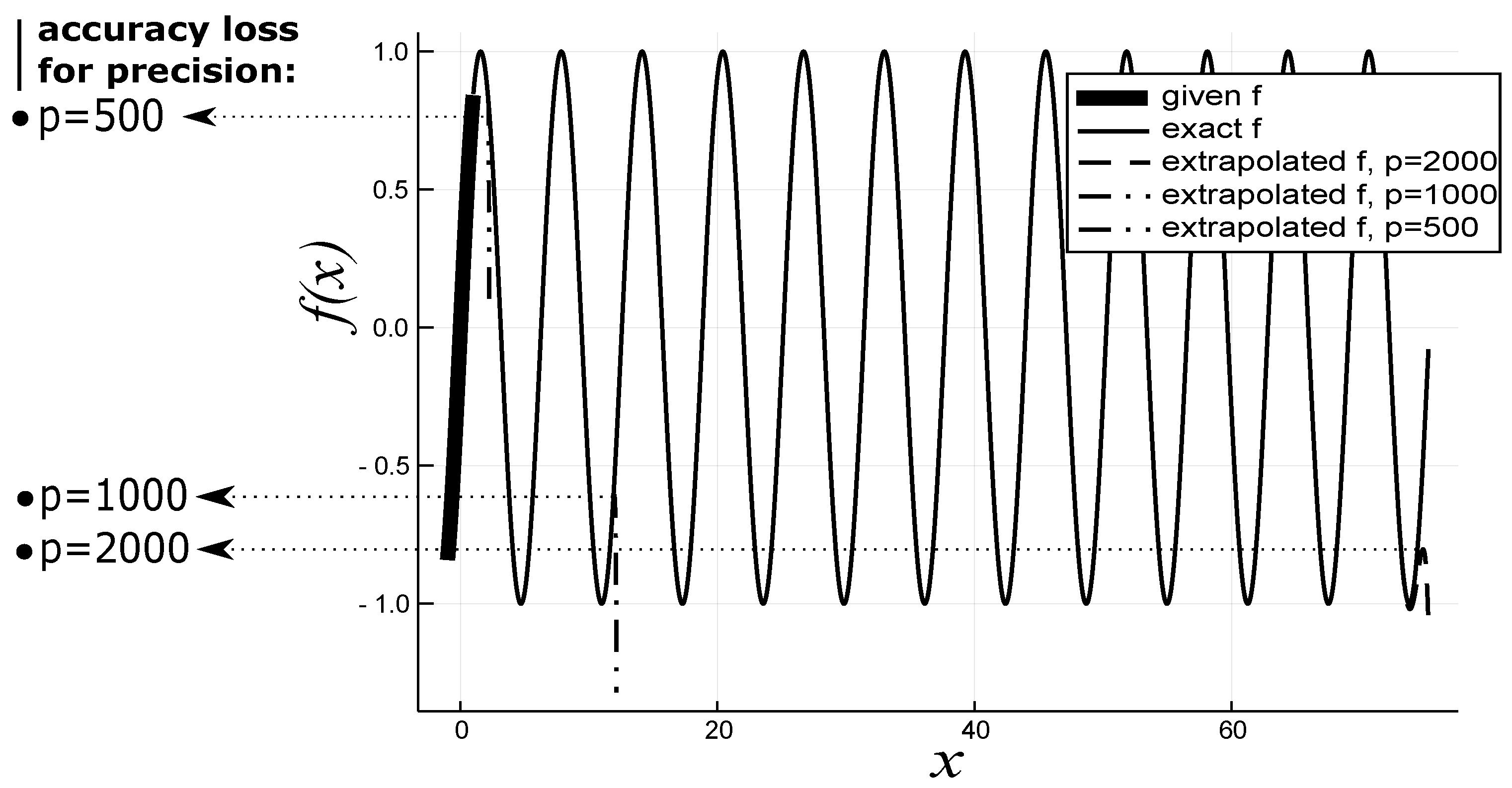
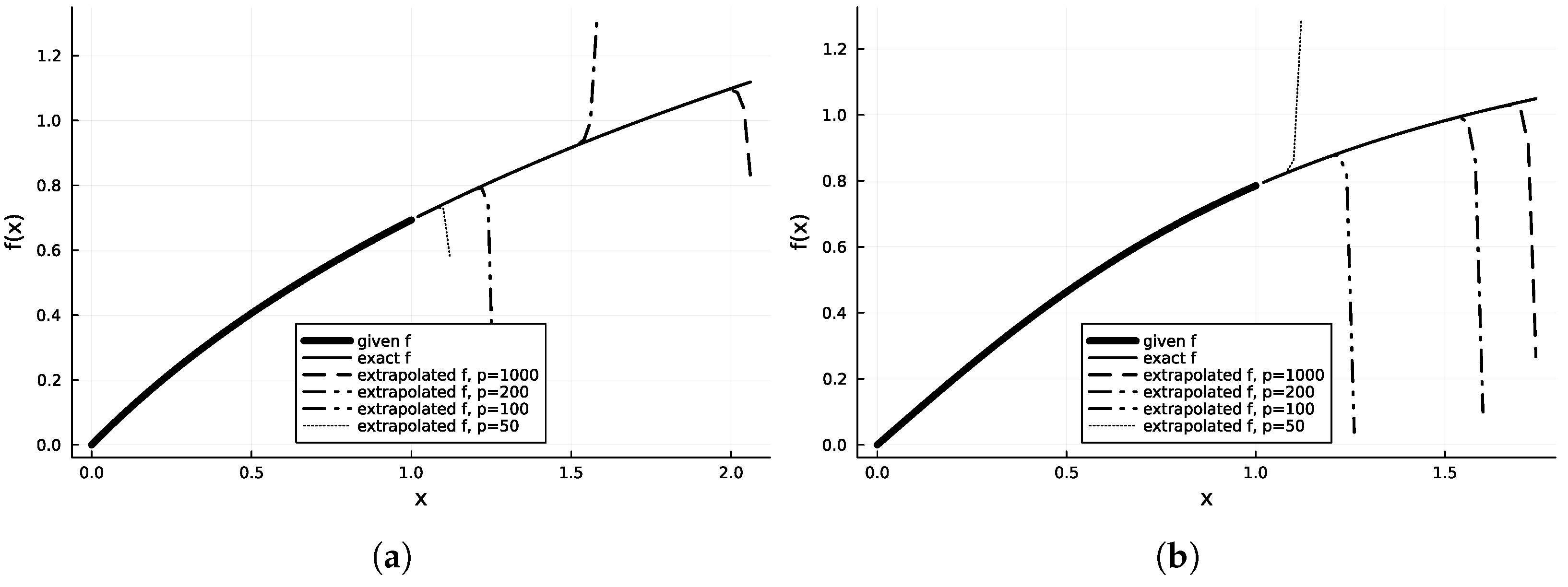
As f ( x ) = sin ( x ) , we have that f n + 1 ( x ) 1 ; hence, the theoretical remainder of the approximation, when using n = 200 terms of the Taylor series, is bounded by | R n ( x ) | 1 ( n + 1 ) ! | 1 0 | n + 1 = 6.308 × 10 378 . In Table 2, the differences among computed and analytical values of f at x and x i = x + d x / 2 are presented.
Interestingly, although for p = 50 , the approximation error for f ( x ) on the given points x is 1.708 × 10 12 , the corresponding interpolation error on x i is 5.932 × 10 8 (Table 2). However, the Runge phenomenon, which is severe at the boundaries, is eliminated for p > 500 .

3.3. Extrapolation

The extrapolation problem of given data is a highly unstable process [33]. Recent results have highlighted the ability of extended spans when using a high arithmetic precision [1]. In Figure 3, the highly extended extrapolation span for f ( x ) = sin ( x ) is depicted. The extrapolation errors start becoming visible only for x > 73 L . We should highlight that this is consistent with the corresponding theory as, for this function, the computed 1 / r = lim sup n | a n | n takes the values of 0.0178, 0.0169, 0.0161, 0.0152, 0.0145, and 0.0137 for the higher values of n (Figure 2a). Accordingly, we may write that r = 1 / 0.0137 72.99 , which is equal to the observed extrapolation span. Accordingly, the extrapolation lengths for p = 1000 are 12.141 according to the root test 1 / r , and in the actual computations, the errors are >1 for x > 12.150 ; and similarly, for p = 500 , the root test value is 2.154 and the computed value is 2.230 , as illustrated in Figure 3. Hence, interestingly, utilizing this approach, we may predict not only determine the behavior of the approximated unknown function within the given domain, but its extrapolation spans as well, and, hence, the prediction ability.
Furthermore, in Figure 4, the extrapolation of f ( x ) = l n ( x + 1 ) (a) and f ( x ) = a r c t a n ( x ) (b) is illustrated by varying the precision p employed in the calculations. In both cases, when utilizing the standard precision p = 50 , the extrapolation span is very short, in contrast to increased precision, such as p = 100 , p = 200 , and p = 1000 .

3.4. Numerical Integration

We calculated the vector a ; hence, we know an approximation of f ( x ) a 0 + a 1 x + a 2 x 2 + + a n x n . By integrating the Taylor polynomial of f, the indefinite integral is
F ( x ) a 0 x + a 1 x 2 2 + a 2 x 3 3 + + a n x n + 1 n + 1 + c .
The only unknown quantity is c, which may be calculated by the supplementary constraint that F ( L ) = 0 ; hence, c a 0 L a 1 L 2 2 a 2 L 3 3 a n L n + 1 n + 1 . f ( x ) = sin ( x ) , hence F ( x ) = cos ( x ) . The proposed scheme offers a direct computation of the integrals, as the vector a is known. In Table 3, the very low errors of numerical integration are demonstrated, as well as the significance of the studied digits. The numerical integration errors in Table 3 are computed as e = F a n F n u , where F a n is the analytical computation F a n = L L f ( x ) d x = cos ( L ) + cos ( L ) = 0 , for the case of s i n ( x ) , and F n u is the corresponding numerical computation, utilizing the computed a .

3.5. Numerical Differentiation

The derivatives of f are directly computed by
a = a 1 , a 2 , , a n = f ( x 0 ) , f ( x 0 ) 1 ! , f ( x 0 ) 2 ! , , f ( n ) ( x 0 ) n ! = df n ! ,
with df denoting the vector of the n ordinary derivatives of f and n ! denoting the vector of the n factorials. The k t h < n derivative at any other point x x 0 may easily be computed by Equation (1), deriving f ( x ) 0 + a 1 + 2 a 2 x + 3 a 3 x 2 + + n a n x n 1 , f ( x ) 0 + 0 + 2 a 2 + 6 a 3 x + + ( n 1 ) n a n x n 2 , and, hence,
f ( k ) ( x ) k ! a k x k + + n ! ( n k ) ! a n x n k ,
where the factors a k , a k + 1 , , a n have already been computed by a . We demonstrate the efficiency of the numerical differentiation in the following example apropos the solution of differential Equations.

3.6. Solution of Ordinary Differential Equations (ODEs)

The solution we investigate utilizes the constitution of the matrices representing the derivatives of each element of V in HAP. For example:
dV = 0 1 2 x 1 ( n 1 ) x 1 n 2 0 1 2 x 2 ( n 1 ) x 2 n 2 0 1 2 x 3 ( n 1 ) x 3 n 2 0 1 2 x n ( n 1 ) x n n 2 , and d 2 V = 0 0 2 ( n 1 ) ( n 2 ) x 1 n 3 0 0 2 ( n 1 ) ( n 2 ) x 2 n 3 0 0 2 ( n 1 ) ( n 2 ) x 3 n 3 0 0 2 ( n 1 ) ( n 2 ) x n n 3 ,
and so on. By utilizing such matrices, we can easily constitute a system of equations representing the differential equation at points x i . To demonstrate the unified approach to the solution of differential equations, we consider the bending of a simply supported beam [34], with the governing equation given below:
E I d 4 w d x 4 = q ( x )
where E is the modulus of elasticity, I the moment of inertia, w the sought solution representing the deflection of the beam, and q the external load. For E = I = L = 1 , q ( x ) = 0 , and fixed boundary conditions w ( 0 ) = 0 , d w d x x = o = 0 , w ( L ) = 1 / 100 , d w d x x = L = 0 , we may write Equation (3) supplemented by the boundary conditions in matrix form as follows:
0 0 0 0 24 ( n 1 ) ( n 2 ) ( n 3 ) ( n 4 ) x 1 n 5 0 0 0 0 24 ( n 1 ) ( n 2 ) ( n 3 ) ( n 4 ) x 2 n 5 0 0 0 0 24 ( n 1 ) ( n 2 ) ( n 3 ) ( n 4 ) x 3 n 5 0 0 0 0 24 ( n 1 ) ( n 2 ) ( n 3 ) ( n 4 ) x n n 5 1 0 0 0 0 0 0 1 0 0 0 0 L 0 0 0 0 0 0 L 0 0 0 0 a 0 a 1 a 2 a n = p 0 p 1 p 2 p n w 0 w 0 w L w L
Solving for a and utilizing matrix V , we derive the sought solution using w = Va . The exact solution is
E I w ( x ) = 2 E I L 3 x 3 + 3 E I L 2 x 2 ,
and, hence, the exact a = 0 , 0 , 3 , 2 , 0 , , 0 . In Figure 5, the ability of a high precision ( p = 1000 ) to identify the exact weights a is revealed, while the p = 50 bits accuracy fails dramatically for such identification. However, they exhibit a lower deviation than the interpolation problem, probably due to the imposition of the boundary conditions.

3.7. System Identification

The inverse problems, that is, the identification of the system which produced a governing differential law [35], is of great interest as this law rigorously describes the behavior of a studied system. We demonstrate the ability of high-precision Taylor polynomials to perform a rapid and precise identification of unknown systems.
Let t be an input variable and s a measured response. As presented above, we may easily compute a = a 1 , a 2 , , a n , by a = V 1 s . Here, we assume the existence of a differential operator T, such that T ( s ) = c . According to [35], we may write T as a power series as T ( s ) = i , j , k = 0 2 b i j k s i s ˙ j s ¨ k = b 000 + b 100 s + b 010 s ˙ + b 001 s ¨ + b 200 s 2 + b 110 s s ˙ + b 101 s s ¨ + b 020 s ˙ 2 + b 011 s ˙ s ¨ + b 002 s ¨ 2 and by setting c = c b 000 ; and assuming a linear approximation, we derive
1 = b 100 s + b 010 s ˙ + b 001 s ¨ c .
Applying the later for all x i and writing the resulting system in matrix form, we obtain
[ Va + dVa + d 2 Va ] b T = 1 ,
where 1 = 1 , 1 , , 1 . Solving for b , we obtain the weights of the derivatives in the differential operator T ( s ) .
For example, if we apply the previous for data of Newton’s second law [30] of motion s ( t ) = t 2 , with s indicating space and t time, we may calculate vectors a and solve Equation (4) for b ; with c = 1 and a p = 1000 bits precision, we derive that b = 0 , 0 , 1 / 2 + O ( 10 270 ) , and, hence, 1 2 s ¨ = 1 s ¨ = 2 , which is equivalent to s ¨ = a , where a = F m = 2 , which represents the external source that produces s ( t ) = t 2 .
We assume that 1 = b 100 s + b 010 s ˙ + b 001 s ¨ ; hence, by integrating s twice, with S = s and S S = s , and utilizing the interval [ 0 , t ] , we obtain t + c 1 = b 100 ( S ( t ) S ( 0 ) ) + b 010 ( s ( t ) s ( 0 ) ) + b 001 ( s ˙ ( t ) s ˙ ( 0 ) ) ; however, S ( 0 ) = s ( 0 ) = s ˙ ( 0 ) = 0 . Accordingly, we may write t = b 100 S ( t ) + b 010 s ( t ) + b 001 s ˙ ( t ) , and if we integrate for a second time in the interval [ 0 , t ] , we obtain
t 2 2 = b 100 ( S S ( t ) S S ( 0 ) ) + b 010 ( S ( t ) S ( 0 ) ) + b 001 ( s ( t ) s ( 0 ) ) ,
and by using S S ( 0 ) = 0 , we obtain
s ( t ) = t 2 2 b 100 S S ( t ) b 010 S ( t ) b 001
The integrals of s, s , and s can be approximated with a high accuracy by utilizing, accordingly, the procedure discussed in Section 3.4, by using the integrals of the obtained Taylor polynomials,
s a 0 t + a 1 t 2 2 + a 2 t 3 3 + + a n t n + 1 n + 1
s a 0 t 2 2 + a 1 t 3 6 + a 2 t 4 12 + + a n t n + 2 ( n + 1 ) ( n + 2 ) ,
as well as the corresponding matrices for all the given t i ,
IV = 1 1 / 2 t 1 / 3 t 1 n + 1 / ( n + 1 ) 1 1 / 2 t 2 / 3 t 2 n + 1 / ( n + 1 ) 1 1 / 2 t 3 / 3 t 3 n + 1 / ( n + 1 ) 1 1 / 2 t n / 3 t n n + 1 / ( n + 1 )
IIV = 1 / 2 1 / 6 t 1 / 12 t 1 n + 2 / ( n + 1 ) / ( n + 2 ) 1 / 2 1 / 6 t 2 / 12 t 2 n + 2 / ( n + 1 ) / ( n + 2 ) 1 / 2 1 / 6 t 3 / 12 t 3 n + 2 / ( n + 1 ) / ( n + 2 ) 1 / 2 1 / 6 t n / 12 t n n + 2 / ( n + 1 ) / ( n + 2 ) .
The calculated impact of b 001 for the p = 50 and p = 1000 bits accuracy is revealed by the resulting extrapolation curves beyond the observed domain, utilizing Equation (5). For the p = 50 bits accuracy, for given data in the domain [ 0 , 1 ] , we may extrapolate only up to a short time ( t = 1.343 ) after the last given t e n d = 1.000 , with threshold for errors < 1.000 , while for p = 2000 bits, the corresponding t attains the remarkably high value of 9.621 × 10 + 10 , highlighting the extrapolation power of high arithmetic precision.

4. Functions in Multiple Dimensions

4.1. Multidimensional Interpolation

The Taylor series of f ( x , y ) , depending on two variables x , y Ω , where Ω is a closed disk about the center x 0 , y 0 , may be written utilizing the partial derivatives of f [31,32] in the form of f ( x , y ) = f ( a , b ) + ( x a ) f x ( a , b ) + ( y b ) f y ( a , b ) + 1 2 ! ( ( x a ) 2 f x x ( a , b ) + 2 ( x a ) ( y b ) f x y ( a , b ) + ( y b ) 2 f y y ( a , b ) ) + , which, in vector form, is written as
f ( x ) = f ( x 0 ) + ( x x 0 ) T D f ( x 0 ) + 1 2 ! ( x x 0 ) T D 2 f ( x 0 ) ( x x 0 ) + ,
where D 2 f ( x 0 ) is the Hessian matrix at x 0 .
Let n be the number of given points of f ( x i , y j ) , with i , j ( 1 , 2 , , n ) . In order to constitute the approximating polynomial of f ( x , y ) with high-order terms and formulate the V matrix with dimensions n × n , we consider all possible combinations of n i , n j ( 0 , 1 , , n 1 ) n i + n j n 1 . Hence, we may write the following for all the given x i :
V ( x i , y j ) = 1 x 1 y 1 x 1 y 1 x 1 2 y 1 2 x 1 n k y 1 n l 1 x 2 y 2 x 2 y 2 x 2 2 y 2 2 x 2 n k y 2 n l 1 x n y n x n y n x n 2 y n 2 x n n k y n n l ,
with k + l = n 1 . Thus, we can approximate f with n polynomial terms using the following:
f = Va a = V 1 f
The computation of a with Equation (6) permits the computation of f ( x i , y j ) , for any x i , y j Ω , by utilizing the corresponding V .
Let f ( x , y ) = sin ( 5 x ) + cos ( e 2 y ) . We approximate f with n = 300 random values x i , y i 0.5 , 0.5 , and, later, we interpolate f with n = 300 random values x i , y j i 0.35 , 0.35 . In Figure 6, the exact and approximated values f ( x i , y j ) are depicted for p = 2000 and p = 50 bits accuracies. Apparently, for the same interpolation problem formulation in three dimensions, the computational precision p dramatically affects the results. The
max f ( x i , y j ) a n a l y t i c a l f ( x i , y j ) n u m e r i c a l
equals 8.570 × 10 09 for p = 2000 and 1.286 × 10 + 01 for p = 50 bits. The polynomials’ weights a were calculated by first computing V 1 by solving V I ; hence, a = V 1 f because a = V I exhibits significant errors. The calculation of the inverse of generic matrices, as well as the solution of systems of Equations in a high precision, is a topic for future research.

4.2. Solution of Partial Differential Equations

We present the ability of a high precision to solve partial differential equations by considering a plate without axial deformations and vertical load q ( x , y ) . The governing Equation [36] has the following form:
4 w x 4 + 2 4 w x 2 y 2 + 4 w y 4 = q D
that is, 2 2 w = q D , where D : = E h 3 12 ( 1 ν 2 ) , E is the modulus of elasticity, v is the Poisson constant, and h is the slab’s height.
The sought solution w ( x , y ) is the slab’s deformation within the boundary conditions w b ( x b , y b ) along some boundaries b = 1 , 2 , . In order to solve Equation (7), we approximate
w = Va
using the approximation scheme of Equation (6), and as the vector a is constant, we obtain w x 4 = V x 4 a , w y 4 = V y 4 a , and w x 2 y 2 = V x 2 y 2 a , with w x k y l denoting the partial derivative of w of order k over x and l over y, k + l w x k y l , for all given x i , y j with i , j ( 1 , 2 , , n ) . Utilizing this notation, we may write Equation (7) for all x i , y j in matrix form as
V x 4 + 2 V x 2 y 2 + V y 4 a = q .
By applying some boundary conditions, we may write for the same a ,
V x 4 + 2 V x 2 y 2 + V y 4 V ( x 1 , y 1 ) V x ( x 2 , y 2 ) × a = q w ( x 1 , y 1 ) w x ( x 1 , y 1 )
a = V x 4 + 2 V x 2 y 2 + V y 4 V ( x 1 , y 1 ) V x ( x 2 , y 2 ) 1 × q w ( x 1 , y 1 ) w x ( x 1 , y 1 ) .
By computing a , we then obtain the sought solution as w = Va .
For example, for a simply supported slab, the boundary conditions are w ( x b , y b ) = w b for some boundary b. We consider a square slab, with n = 20 divisions per dimension, d x = 1 / 99 , L = ( n 1 ) d x , and w ( x b , y b ) = 0 , at the four linear boundaries, and q = 1 , the normalized load to comprise values of 1 everywhere (Equation (7)). After the computation of a with Equation (8), we may easily compute the corresponding shear forces, which are defined by
Q x = D x 2 w x 2 + 2 w y 2 , Q y = D y 2 w x 2 + 2 w y 2 .
We utilize the computed a and matrices V x x x , V x y y , V y x x , V y y y . Newton’s equilibrium states that the total shear force at the boundaries should be equal to the total applied force. For a constant load over the plate, the Equilibrium error
max A q ( x , y ) Q x , y ,
for p = 50 bits is 6.924 × 10 05 , and for p = 2000 , it is 2.242 × 10 591 . We observe that there is a large difference, though the errors are small, even with p = 50 bits. Interestingly, utilizing a concentrated load by loading the nodes close to ( 0 , 0 ) , the inversion error
max V x 4 + 2 V x 2 y 2 + V y 4 V ( x 1 , y 1 ) V x ( x 2 , y 2 ) 1 × V x 4 + 2 V x 2 y 2 + V y 4 V ( x 1 , y 1 ) V x ( x 2 , y 2 ) I ,
for p = 50 bits is 43.988 , and for p = 2000 , it is 4.381 × 10 587 , further highlighting the significance of accuracy in the calculations.

5. Conclusions

Function approximation exists in the core calculations of computational mechanics, with implications for other disciplines. In this work, a high arithmetic precision, when applied to Taylor polynomials, is found capable of executing various numerical tasks precisely. Particularly, a high arithmetic precision significantly improves accuracy in solving beam deflection equations, demonstrating the importance of computational precision in the solution of ODEs. A high precision significantly enhances the solution accuracy of partial differential equations for slab deformation under a vertical load, highlighting the critical role of computational precision in PDEs. Furthermore, traditional issues like the Runge phenomenon, commonly encountered in numerical approximations, are eliminated with the use of a HAP. The radius of convergence for the Taylor series is precisely computable using a HAP, providing valuable insights into the interpolation accuracy and potential extrapolation range of an unknown function. Overall, the use of Taylor polynomials in a high arithmetic precision showcases potential as a unified approach to various numerical computations, delivering highly accurate results and revealing that some numerical instabilities are due to computational inaccuracies rather than methodological issues. Future research can include parallel computing techniques or optimized matrix inversion strategies to deal with the Vandermonde matrix and other related computational challenges in HAP. Taylor polynomials with a high precision could also be applied to more complex systems and geometries in computational mechanics, as well as other engineering problems involving function approximation, such as fluid dynamics and quantum physics. Extending the research to high-dimensional problems where function approximation becomes significantly more complicated could also be an important field, addressing the practical aspects of high-precision calculations for partial differential equations and integral equations in a high-dimensional space. The study of precision in calculations illustrates the odd but fundamental epistemological principle that even 1 + 1 = 2 might be falsified [37].

Funding

We acknowledge support from project “SimEA” funded by the European Union’s Horizon 2020 research and innovation program under Grant Agreement No. 810660.

Data Availability Statement

All the data and results may be reproduced by the computer code on GitHub https://github.com/nbakas/TaylorBigF.jl. The code is in generic form, so as to solve for any numerical problem with the discussed methods. The code is written in Julia [24], utilizing the MPFR [38] and GMP [9] Libraries.

Conflicts of Interest

The author declares no conflict of interest.

Nomenclature

xVariable x, corresponding to f ( x )
x 0 Initial point in the approximation
nNumber of terms in the Taylor series, also number of nodes
LLength of the given domain
EModulus of elasticity
IInertia of the beam
f ( x ) Analytic function
f Vector of function values
x Vector of points
rRadius of convergence
V Vandermonde matrix
df Vector of the derivatives of the function f ( x )
DFlexural rigidity of plate
wDeflection of the beam/plate
qExternal load of beam/plate
a Coefficient vector for Taylor polynomials
vPoisson constant
hSlab’s thickness

References

  1. Bakas, N.P. Numerical Solution for the Extrapolation Problem of Analytic Functions. Research 2019, 2019, 3903187. [Google Scholar] [CrossRef]
  2. Bailey, D.H.; Jeyabalan, K.; Li, X.S. A comparison of three high-precision quadrature schemes. Exp. Math. 2005, 14, 317–329. [Google Scholar] [CrossRef]
  3. Cheng, A.H. Multiquadric and its shape parameter—A numerical investigation of error estimate, condition number, and round-off error by arbitrary precision computation. Eng. Anal. Bound. Elem. 2012, 36, 220–239. [Google Scholar] [CrossRef]
  4. Huang, C.S.; Lee, C.F.; Cheng, A.H. Error estimate, optimal shape factor, and high precision computation of multiquadric collocation method. Eng. Anal. Bound. Elem. 2007, 31, 614–623. [Google Scholar] [CrossRef]
  5. Sharma, N.N.; Jain, R.; Pokkuluri, M.M.; Patkar, S.B.; Leupers, R.; Nikhil, R.S.; Merchant, F. CLARINET: A quire-enabled RISC-V-based framework for posit arithmetic empiricism. J. Syst. Archit. 2023, 135, 102801. [Google Scholar] [CrossRef]
  6. Lei, X.; Gu, T.; Xu, X. ddRingAllreduce: A high-precision RingAllreduce algorithm. CCF Trans. High Perform. Comput. 2023, 5, 245–257. [Google Scholar] [CrossRef]
  7. Wu, C.; Xia, Y.; Xu, Z.; Liu, L.; Tang, X.; Chen, Q.; Xu, F. Mathematical modelling for high precision ray tracing in optical design. Appl. Math. Model. 2024, 128, 103–122. [Google Scholar] [CrossRef]
  8. Friebel, K.F.A.; Bi, J.; Castrillon, J. Base2: An IR for Binary Numeral Types. In Proceedings of the 13th International Symposium on Highly Efficient Accelerators and Reconfigurable Technologies, Kusatsu, Japan, 14–16 June 2023; pp. 19–26. [Google Scholar] [CrossRef]
  9. Granlund, T. The GNU Multiple Precision Arithmetic Library. Free Softw. Found. Available online: https://gmplib.org/ (accessed on 13 January 2024).
  10. Amato, G.; Scozzari, F. JGMP: Java bindings and wrappers for the GMP library. SoftwareX 2023, 23, 101428. [Google Scholar] [CrossRef]
  11. Guessab, A.; Nouisser, O.; Schmeisser, G. Multivariate approximation by a combination of modified Taylor polynomials. J. Comput. Appl. Math. 2006, 196, 162–179. [Google Scholar] [CrossRef]
  12. Kalantari, B. Generalization of Taylor’s theorem and Newton’s method via a new family of determinantal interpolation formulas and its applications. J. Comput. Appl. Math. 2000, 126, 287–318. [Google Scholar] [CrossRef]
  13. Berz, M.; Makino, K. Verified Integration of ODEs and Flows Using Differential Algebraic Methods on High-Order Taylor Models. Reliab. Comput. 1998, 10, 361–369. [Google Scholar] [CrossRef]
  14. Yalçinbaş, S.; Sezer, M. The approximate solution of high-order linear Volterra-Fredholm integro-differential equations in terms of Taylor polynomials. Appl. Math. Comput. 2000, 112, 291–308. [Google Scholar] [CrossRef]
  15. Ranjan, R.; Prasad, H.S. A novel approach for the numerical approximation to the solution of singularly perturbed differential-difference equations with small shifts. J. Appl. Math. Comput. 2021, 65, 403–427. [Google Scholar] [CrossRef]
  16. Platte, R.B.; Trefethen, L.N.; Kuijlaars, A.B.J. Impossibility of Fast Stable Approximation of Analytic Functions from Equispaced Samples. SIAM Rev. 2011, 53, 308–318. [Google Scholar] [CrossRef]
  17. Boyd, J.P. Defeating the Runge phenomenon for equispaced polynomial interpolation via Tikhonov regularization. Appl. Math. Lett. 1992, 5, 57–59. [Google Scholar] [CrossRef]
  18. Zhang, S.Q.; Fu, C.H.; Zhao, X.D. Study of regional geomagnetic model of Fujian and adjacent areas based on 3D Taylor Polynomial model. Acta Geophys. Sin. 2016, 59, 1948–1956. [Google Scholar] [CrossRef]
  19. Boyd, J.P.; Xu, F. Divergence (Runge Phenomenon) for least-squares polynomial approximation on an equispaced grid and Mock-Chebyshev subset interpolation. Appl. Math. Comput. 2009, 210, 158–168. [Google Scholar] [CrossRef]
  20. Boyd, J.P.; Ong, J.R. Exponentially-convergent strategies for defeating the runge phenomenon for the approximation of non-periodic functions, part I: Single-interval schemes. Commun. Comput. Phys. 2009, 5, 484–497. [Google Scholar]
  21. Taylor, B. Principles of Linear Perspective; Knaplock, R., Ed.; British Library: London, UK, 1715. [Google Scholar]
  22. Babouskos, N.G.; Katsikadelis, J.T. Optimum design of thin plates via frequency optimization using BEM. Arch. Appl. Mech. 2015, 85, 1175–1190. [Google Scholar] [CrossRef]
  23. Yiotis, A.J.; Katsikadelis, J.T. Buckling of cylindrical shell panels: A MAEM solution. Arch. Appl. Mech. 2015, 85, 1545–1557. [Google Scholar] [CrossRef]
  24. Bezanson, J.; Edelman, A.; Karpinski, S.; Shah, V.B. Julia: A fresh approach to numerical computing. SIAM Rev. 2017, 59, 65–98. [Google Scholar] [CrossRef]
  25. Apostol, T.M. Calculus; John Wiley & Sons: Hoboken, NJ, USA, 1967. [Google Scholar]
  26. Browder, A. Mathematical Analysis: An Introduction; Springer Science & Business Media: Berlin/Heidelberg, Germany, 2012. [Google Scholar]
  27. Katsoprinakis, E.S.; Nestoridis, V.N. Partial sums of Taylor series on a circle. Ann. L’Institut Fourier 2011, 39, 715–736. [Google Scholar] [CrossRef]
  28. Nestoridis, V. Universal Taylor series. Ann. de L’Institut Fourier 2011, 46, 1293–1306. [Google Scholar] [CrossRef]
  29. Press, W.H.; Teukolsky, S.A. VWT, and FBP, Numerical Recipes: The Art of Scientific Computing; Cambridge University Press: Cambridge, UK, 2007. [Google Scholar]
  30. Horn, R.A.; Johnson, C.R. Topics in Matrix Analysis; Cambridge University Press: Cambridge, UK, 1991. [Google Scholar]
  31. Ycart, B. A case of mathematical eponymy: The Vandermonde determinant. arXiv 2012, arXiv:1204.4716. [Google Scholar] [CrossRef]
  32. Turner, L.R. Inverse of the Vandermonde Matrix with Applications; NASA–TN D-3547; NASA: Washington, DC, USA, 1966.
  33. Demanet, L.; Townsend, A. Stable extrapolation of analytic functions. Found. Comput. Math. 2019, 19, 297–331. [Google Scholar] [CrossRef]
  34. Boresi, A.P.; Sidebottom, O.M.; Saunders, H. Advanced Mechanics of Materials (4th Ed.). J. Vib. Acoust. Stress Reliab. Des. 1988, 110, 256–257. [Google Scholar] [CrossRef]
  35. Katsikadelis, J.T. System identification by the analog equation method. WIT Trans. Model. Simul. 1995, 10, 12. [Google Scholar]
  36. Katsikadelis, J.T. The Boundary Element Method for Plate Analysis; Elsevier: Amsterdam, The Netherlands, 2014. [Google Scholar]
  37. Gregory, F.H. Arithmetic and Reality: A Development of Popper’s Ideas. Philos. Math. Educ. J. 2011, 26. [Google Scholar]
  38. Fousse, L.; Hanrot, G.; Lefèvre, V.; Pélissier, P.; Zimmermann, P. MPFR: A multiple-precision binary floating-point library with correct rounding. ACM Trans. Math. Softw. 2007, 33, 2. [Google Scholar] [CrossRef]
Figure 1. Given values of f ( x ) at points x i for the approximation of f by inverting the corresponding Vandermonde matrix V .
Computation 12 00053 g001
Figure 2. Radius of convergence for the computed Taylor expansion of f ( x ) = sin ( x ) for the same domain and different computational precisions. (a) p = 2000 bits (b) p = 50 bits.
Computation 12 00053 g002
Figure 3. Extrapolation of f for varying values of arithmetic precision p. For p = 2000 , the extrapolation errors are visible only for x > 73 L without any periodicity information given.
Computation 12 00053 g003
Figure 4. Extrapolation of (a) f ( x ) = l n ( x + 1 ) and (b) f ( x ) = a r c t a n ( x ) for varying values of precision p.
Computation 12 00053 g004
Figure 5. Calculated a for p = 50 and p = 1000 bits accuracies. Low arithmetic precision yields incorrect coefficients a for the same problem and data.
Computation 12 00053 g005
Figure 6. Exact and approximated values of f for precision p = 2000 bits (a) and p = 50 bits (b). We can observe that by utilizing enough digits, we have a precise approximation in contrast to a standard precision, indicating a computational deficiency and not a methodological one.
Computation 12 00053 g006
Table 1. Variation of V 1 , det ( V ) , and a , with the calculation precision in bits p, for the same example.
Error vs. Precision (p) p = 50 p = 100 p = 500 p = 1000 p = 2000
det V a n det V n u 3.866 × 10 2341 4.300 × 10 4106 2.735 × 10 6810 3.741 × 10 6960 1.853 × 10 7261
max | V a n 1 V n u 1 | 9.739 × 10 100 4.911 × 10 94 1.242 × 10 38 1.124 × 10 111 5.504 × 10 413
max | a a n a n u | 4.029 × 10 1 1.813 × 10 0 9.252 × 10 18 9.252 × 10 18 9.252 × 10 18
Table 2. Variation of approximation errors with the calculation precision in bits p.
Error vs. Precision (p) p = 50 p = 100 p = 500 p = 1000 p = 2000
max | f a n ( x ) f n u ( x ) | 1.708 × 10 12 3.045 × 10 28 1.231 × 10 148 3.770 × 10 299 3.475 × 10 600
max | f a n ( x i ) f n u ( x i ) | 5.932 × 10 08 2.045 × 10 15 3.673 × 10 96 2.373 × 10 246 9.909 × 10 407
Table 3. Numerical integration errors.
Error vs. Precision (p) p = 50 p = 100 p = 500 p = 1000 p = 2000
F a n F n u 1.502 × 10 09 3.957 × 10 17 1.226 × 10 97 2.431 × 10 249 1.028 × 10 548
Disclaimer/Publisher’s Note: The statements, opinions and data contained in all publications are solely those of the individual author(s) and contributor(s) and not of MDPI and/or the editor(s). MDPI and/or the editor(s) disclaim responsibility for any injury to people or property resulting from any ideas, methods, instructions or products referred to in the content.

