Algorithm for Propeller Optimization Based on Differential Evolution

Abstract

This paper describes the development of a methodology for air propeller optimization using Bezier curves to describe blade geometry. The proposed approach allows for more flexibility in setting the propeller shape, for example, using a variable airfoil over the blade span. The goal of optimization is to identify the appropriate geometry of a propeller that reduces the power required to achieve a given thrust. Because the proposed optimization problem is a constrained optimization process, the technique of generating a penalty function was used to convert the process into a nonconstrained optimization. For the optimization process, a variant of the differential evolution algorithm was used, which includes adaptive techniques of the evolutionary operators and a population size reduction method. The aerodynamic characteristics of the propellers were obtained using the similar to blade element momentum theory (BEMT) isolated section method (ISM) and the XFOIL program. Replacing the angle of geometric twist with the angle of attack of the airfoil section as a design variable made it possible to increase the robustness of the optimization algorithm and reduce the calculation time. The optimization technique was implemented in the OpenVINT code and has been used to design helicopter and tractor propellers for unmanned aerial vehicles. The development algorithm was validated experimentally and using CFD numerical method. The experimental tests confirm that the optimized propeller geometry is superior to commercial analogues available on the market.

1. Introduction

The propeller is one of the most important elements of an aircraft that provides lift and propulsion in the air. The relevance of propellers as a propulsion system has increased with the current growth in the production of unmanned aerial vehicles for various purposes around the world. The air propeller’s design is an important part of aircraft design, beginning from the conceptual design stage [1]. An optimized propeller can significantly reduce emissions, improve acoustic response, and enhance performance [2]. The design of air propellers to minimize propulsion system energy costs began with Zhukovsky, Betz, and Goldstein [3,4] and was then refined by other scientists [5,6,7,8].

Propeller optimization is a complex, often multi-objective problem that requires consideration of many factors and constraints, including aerodynamic issues, strength, and acoustics [7,9,10,11,12]. The most common goals of propeller optimization from an aerodynamic perspective are the requirements of maximum thrust, maximum efficiency, and a balanced propeller based on Paretto optimality [13,14,15].

In recent years, computational fluid dynamics (CFD) using computer-aided engineering (CAE) systems has become an important method for propeller design and computation [16,17,18]. Therefore, the use of the finite volume method is irrational because it requires large computational power. Some of the most commonly used propeller aerodynamic characteristics calculation methods currently are Blade Element Method (BEM), Blade Element Momentum Theory (BEMT), Vortex Lattice Method (VLM), and Computational Fluid Dynamics (CFD) [1,19]. For tip-loss correction, different methods are used [20], including the Goldstein function [21] and Glauert correction [22,23,24]. The BEM and BEMT methods, due to the fast calculation, have been the most used in optimization processes. The Isolated Section Method (ISM) is similar to BEMT method, based on the Zhukovsky propeller vortex theory, using the Goldstein function for tip-loss correction [25,26]. It should be noted that the accuracy of the BEM, BEMT and ISM methods depends on the precision of the propeller’s cross-sections aerodynamic coefficients prediction. XFOIL code [27] based on the discrete vortex method is a common technique for predicting the airfoils aerodynamic characteristics in propeller design [24,28].

The methodology of propeller geometry parametrization is part of its the aerodynamic optimization problem. Bezier surfaces and curves have the possibility of generating complex shapes using some control points [29]. This feature makes the use of Bezier curves and surfaces suitable for describing propeller cross-sections (airfoils [30,31,32]) and the propeller blades in general, including chord and twist [1,33]. Due to the reduced number of control points, these curves and surfaces are used in propeller shape optimization processes [34], especially when used in conjunction with evolutionary algorithms [35,36] and artificial neural networks [1,33].

Various methods are used in solving the propeller optimization problem. The authors of [37] solved a multi-objective optimization problem subject to a set of constraints using a direct search algorithm. The paper [28] describes the experimental verification and application of a method of multi-criteria optimization using genetic algorithms for the design of a propeller for a high-altitude aircraft. The articles [38,39] discuss the effectiveness of differential evolution-based algorithms for optimizing the shape of different types of propellers.

BEMT and IMS methods for calculating a given shape propeller aerodynamic performance require an airfoil angle of attack selection cycle, causing the need for an airfoil drag polar calculation database [40] and drag curve extrapolation when the geometric twist exceeds the limits on angles of attack. Replacing the twist angle in the design variables with the angle of attack allows the optimization process to immediately search for the desired airflow field and eliminate an additional cycle of searching for the angle of attack for each propeller individual. In the current work, a modification of ISM consists in the airfoil effective angle usage instead of the geometrical twist angle is presented. The geometric twist is calculated for the optimum propeller when the optimum distribution of the angle of attack over the span is found. This approach also improves the robustness of the optimization process by directly controlling the constraints imposed on the angle of attack.

The parametric geometric model of the propeller used in the current work implements Bezier curves to specify the dependencies of the parameters of thickness, curvature, and positions of the maximum thickness and maximum curvature of the airfoil along the blade span. This makes it possible to use different thicknesses and curvatures of airfoils along the blade span, which allows the aerodynamic twist of the blade to be varied.

In addition, the article considers the use of interpolation of the calculation of the aerodynamic characteristics of the airfoils on the blade span, which also allows to accelerate the process.

The techniques of parameterization of propeller geometry, calculation of its aerodynamic characteristics and optimization of its shape considered in the paper are implemented in the OpenVINT code [41]. This code uses the following techniques: geometry modeling with Bézier curves, a modified ISM for obtaining propeller aerodynamic coefficients based on XFOIL for airfoils characteristics calculation, optimization by an evolutionary algorithm with adaptive techniques, and population size reduction methods.

The structure of this paper is as follows: Section 2 describes the methods that comprise the OpenVINT algorithm; in Section 3, two case studies are described in which the versatility of the algorithm for optimizing different types of propellers is shown; finally, the discussions relevant to the results and conclusions of this work are presented.

2. Methods

2.1. Mathematical Model of Propeller Optimization

The objective of this paper is to develop an algorithm that allows the optimization of propeller geometry to minimize the power required to achieve a given thrust. This translates into improved energy consumption. Mathematically, the optimization problem can be expressed as a constrained optimization problem. This paper describes the development of an optimization algorithm to improve the performance of propellers used in unmanned aerial vehicles.

min W(x),

such that T_obj − T(x) ≤ 0,

x∊X

where W(x) is the required power of the propeller; T(x) is the thrust provided by the propeller; T_obj is the desired thrust; x is the vector of design parameters belonging to the feasible set of solutions X.

For this optimization problem to be solved by evolutionary algorithms, the problem had to be converted into an unconstrained optimization problem. This was achieved by using a penalty function, which will be used as a fitness function. The penalty function is expressed as follows:

$$\mathrm{L}\left(\mathrm{x}\right)=\left\{\begin{array}{cc}\mathrm{W}\left(\mathrm{x}\right)& \mathrm{i}\mathrm{f}\mathsf{\psi }\left(\mathrm{x}\right)=0\\ \mathrm{R}\mathsf{\psi }\left(\mathrm{x}\right)+\mathrm{U}\mathrm{*}& \mathrm{i}\mathrm{f}\mathsf{\psi }\left(\mathrm{x}\right)>0\wedge \mathrm{W}\left(\mathrm{x}\right)\le \mathrm{U}\mathrm{*}\\ \mathrm{R}\mathsf{\psi }\left(\mathrm{x}\right)+\mathrm{W}\left(\mathrm{x}\right)& \mathrm{i}\mathrm{f}\mathsf{\psi }\left(\mathrm{x}\right)>0\wedge \mathrm{W}\left(\mathrm{x}\right)>\mathrm{U}\mathrm{*}\end{array}\right.$$

(1)

where

$$\mathsf{\psi }\left(\mathrm{x}\right)=\max \left\{0,{\mathrm{T}}_{\mathrm{o}\mathrm{b}\mathrm{j}}-\mathrm{T}\left(\mathrm{x}\right)\right\}$$

(2)

where U* is an upper bound on the constrained global minimum value; R is a penalty parameter that allows to equate the values obtained in ψ(x) with U*. A large value is assigned to U* initially, but the value needs to be updated with the current best known function value at feasible points. Hence, the initial U* is not updated until a feasible solution has been found. ψ(x) > 0 only if x is infeasible [42]. Therefore, the optimization problem remains as:

min L(x),

such that x∊X

2.2. Selection of Design Variables

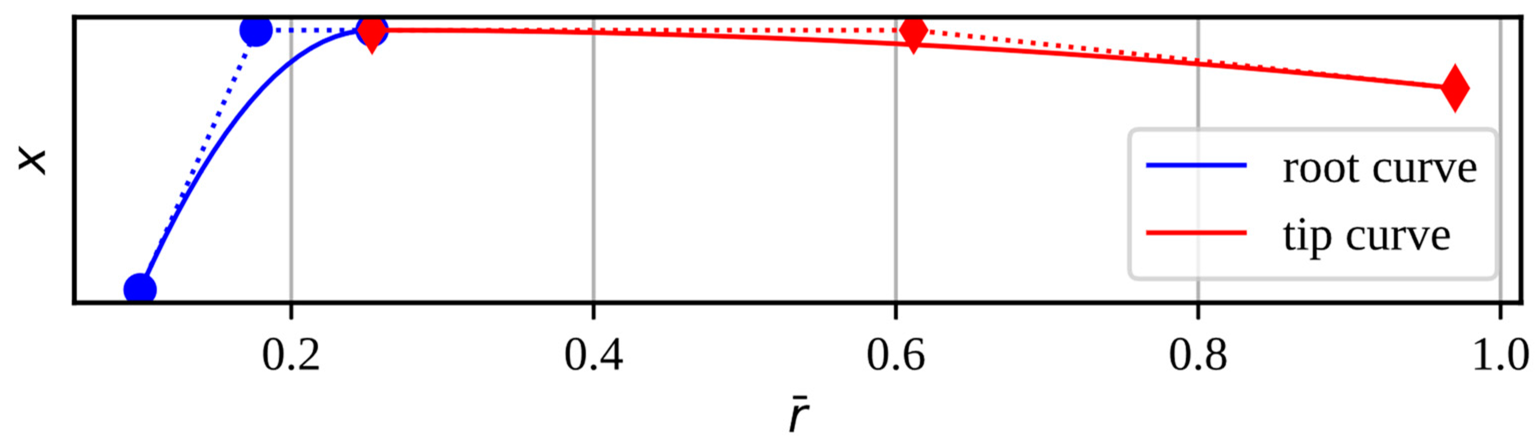
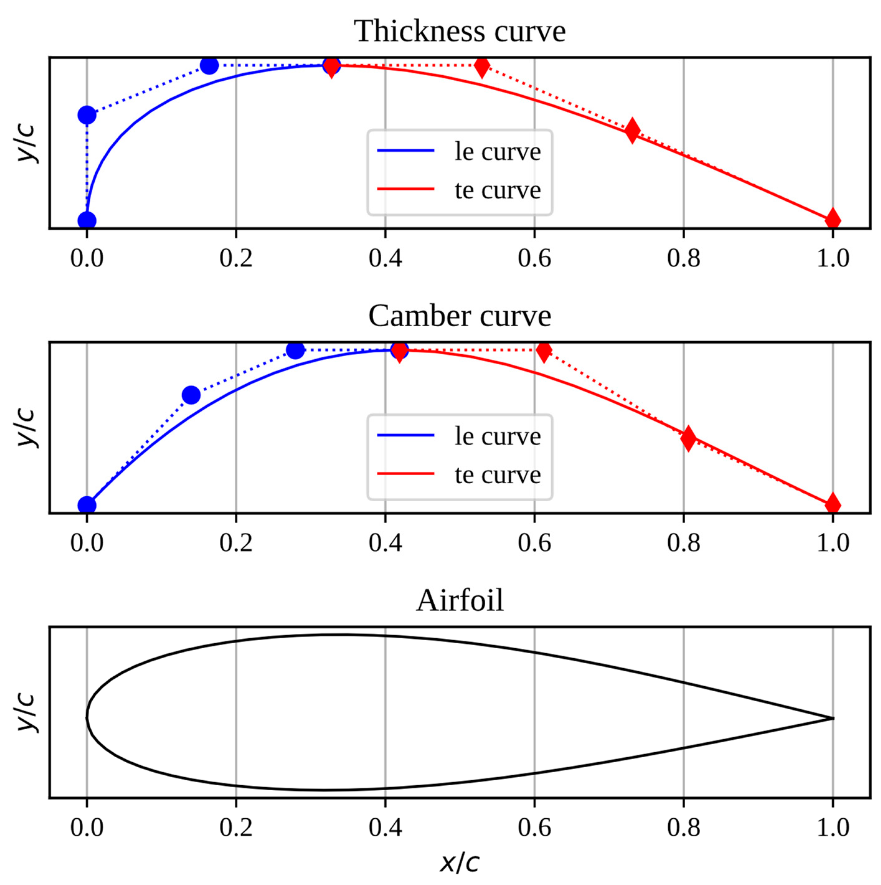
Two types of design variables were proposed: those that describe in a general way the geometry of the propeller or the operation, such as the diameter of the propeller (d, in m), number of blades (B), and number of revolutions per minute (n_m, rev/min); and others that change depending on the radius of the propeller, such as the chord length, effective angle of the airfoil, and the geometry of the airfoil. We considered that these variables have a smooth and continuous variation along the propeller radius using Bezier curves. This variation was achieved using two quadratic Bezier curves [43] (see Figure 1). A quadratic Bezier curve is the path drawn by the following function:

$$\mathrm{B}\mathrm{C}\left(\mathrm{t}\right)=\left(1-{\mathrm{t}}^2\right){\mathrm{P}}_0+2\left(1-\mathrm{t}\right)\mathrm{t}{\mathrm{P}}_1+{\mathrm{t}}^2{\mathrm{P}}_2$$

(3)

where P₀, P₁ and P₂ are control points, and t is a parameter that always varies from 0 to 1.

BC(t) can also be decomposed as (${\mathrm{B}}_{\overline{\mathrm{r}}}$(t), B_x(t)), where $\overline{\mathrm{r}}$ indicates the relative radius of the propeller and x the design parameter.

$${\mathrm{B}}_{\overline{\mathrm{r}}}\left(\mathrm{t}\right)={(1-\mathrm{t})}^2{\overline{\mathrm{r}}}_0+2\left(1-\mathrm{t}\right)\mathrm{t}{\overline{\mathrm{r}}}_1+{\mathrm{t}}^2{\overline{\mathrm{r}}}_2,$$

(4)

$${\mathrm{B}}_{\mathrm{x}}\left(\mathrm{t}\right)={(1-\mathrm{t})}^2{\mathrm{x}}_0+2\left(1-\mathrm{t}\right)\mathrm{t}{\mathrm{x}}_1+{\mathrm{t}}^2{\mathrm{x}}_2,$$

(5)

The control points that determine the Bézier curves for each design variable as a function of the propeller’s relative radius are as follows:

• Root curve

$$\left\{\begin{array}{c}{\overline{\mathrm{r}}}_0^{\mathrm{r}}=0.1\\ {\overline{\mathrm{r}}}_1^{\mathrm{r}}=0.5{\overline{\mathrm{r}}}_{\mathrm{x}\mathrm{m}}+0.05\\ {\overline{\mathrm{r}}}_2^{\mathrm{r}}={\overline{\mathrm{r}}}_{\mathrm{x}\mathrm{m}}\end{array}\right. \left\{\begin{array}{c}{\mathrm{x}}_0^{\mathrm{r}}={\mathrm{x}}_{\mathrm{r}}\\ {\mathrm{x}}_1^{\mathrm{r}}={\mathrm{x}}_{\mathrm{m}}\\ {\mathrm{x}}_2^{\mathrm{r}}={\mathrm{x}}_{\mathrm{m}}\end{array}\right.$$

(6)

• Tip curve

$$\left\{\begin{array}{c}{\overline{\mathrm{r}}}_0^{\mathrm{t}}={\overline{\mathrm{r}}}_{\mathrm{x}\mathrm{m}}\\ {\overline{\mathrm{r}}}_1^{\mathrm{t}}=0.5{\overline{\mathrm{r}}}_{\mathrm{x}\mathrm{m}}+0.485\\ {\overline{\mathrm{r}}}_2^{\mathrm{t}}=0.97\end{array}\right. \left\{\begin{array}{c}{\mathrm{x}}_0^{\mathrm{t}}={\mathrm{x}}_{\mathrm{m}}\\ {\mathrm{x}}_1^{\mathrm{t}}={\mathrm{x}}_{\mathrm{m}}\\ {\mathrm{x}}_2^{\mathrm{t}}={\mathrm{x}}_{\mathrm{t}}\end{array}\right.$$

(7)

In Equations (4)–(7), x may be the chord relative to the propeller diameter (c/d), the effective angle (α), maximum thickness (y_t), position of the maximum thickness relative to the chord (x_t), the maximum camber (y_c), and the position of the maximum camber relative to the chord (x_c). Each of these variables is with respect to the profile of each section of the propeller blade. The variable $\overline{\mathrm{r}}$_xm refers to the union position of the two Bezier curves. The subscripts r, m, t refers to the values of the design variable with respect to 10% of the blade radius, the union point of the Bezier curves, and 97% of the blade radius, respectively. Therefore, each vector of design variables is formed as x_i = [(c/d)_r, (c/d)_m, (c/d)_t, $\overline{\mathrm{r}}$_cm, α_r, α_m, α_t, $\overline{\mathrm{r}}$_αm, y_tr, y_tm, y_tt, $\overline{\mathrm{r}}$_ytm, x_tr, x_tm, x_tt, $\overline{\mathrm{r}}$_xtm, y_cr, y_cm, y_ct, $\overline{\mathrm{r}}$_ycm, x_cr, x_cm, x_ct, $\overline{\mathrm{r}}$_xcm, n_m, B, d]_i.

2.3. Development of the Input Geometry

The Isolated Sections Method (ISM) [44,45] was selected to obtain the aerodynamic characteristics of the different propeller configurations. This method requires knowledge of the geometry, chord, and effective angle of attack of the airfoil in different sections of the propeller blade. The chord values and the effective angle of attack were obtained by constructing the distribution curves (Bezier curve) and using the input parameters (c/d)_r, (c/d)_m, (c/d)_t, $\overline{\mathrm{r}}$_cm, α_r, α_m, α_t, and $\overline{\mathrm{r}}$_αm. To obtain the coordinates of the airfoil in each section, an airfoil parameterization method based on the Bezier-PARSEC technique was proposed [46]. The use of Bezier curves makes it possible to model a wide variety of profile types [39,47]. Each airfoil is constructed with four cubic Bezier curves, two curves for determining the thickness of the airfoil and two curves for determining the camber of the airfoil (see Figure 2).

The parametric functions for determining each cubic Bezier curve are as follows:

$${\mathrm{B}}_{\mathrm{x}}\left(\mathrm{t}\right)={(1-\mathrm{t})}^3{\mathrm{x}}_0+3{(1-\mathrm{t})}^2\mathrm{t}{\mathrm{x}}_1+3(1-\mathrm{t}){\mathrm{t}}^2{\mathrm{x}}_2+{\mathrm{t}}^3{\mathrm{x}}_3,$$

(8)

$${\mathrm{B}}_{\mathrm{y}}\left(\mathrm{t}\right)={(1-\mathrm{t})}^3{\mathrm{y}}_0+3{(1-\mathrm{t})}^2\mathrm{t}{\mathrm{y}}_1+3\left(1-\mathrm{t}\right){\mathrm{t}}^2{\mathrm{y}}_2+{\mathrm{t}}^3{\mathrm{y}}_3,$$

(9)

The construction of the profile is carried out using the following equations:

$${\mathrm{X}}_{\mathrm{t}}={\mathrm{B}}_{\mathrm{x}\mathrm{t}}^{\mathrm{l}\mathrm{e}}\left(\mathrm{t}\right)+{\mathrm{B}}_{\mathrm{x}\mathrm{t}}^{\mathrm{t}\mathrm{e}}\left(\mathrm{t}\right)$$

(10)

$${\mathrm{Y}}_{\mathrm{t}}={\mathrm{B}}_{\mathrm{y}\mathrm{t}}^{\mathrm{l}\mathrm{e}}\left(\mathrm{t}\right)+{\mathrm{B}}_{\mathrm{y}\mathrm{t}}^{\mathrm{t}\mathrm{e}}\left(\mathrm{t}\right)$$

(11)

$${\mathrm{X}}_{\mathrm{c}}={\mathrm{B}}_{\mathrm{x}\mathrm{c}}^{\mathrm{l}\mathrm{e}}\left(\mathrm{t}\right)+{\mathrm{B}}_{\mathrm{x}\mathrm{c}}^{\mathrm{t}\mathrm{e}}\left(\mathrm{t}\right)$$

(12)

$${\mathrm{Y}}_{\mathrm{c}}={\mathrm{B}}_{\mathrm{y}\mathrm{c}}^{\mathrm{l}\mathrm{e}}\left(\mathrm{t}\right)+{\mathrm{B}}_{\mathrm{y}\mathrm{c}}^{\mathrm{t}\mathrm{e}}\left(\mathrm{t}\right)$$

(13)

$$\mathsf{\theta }={\tan }^{-1}\left(\raisebox{1ex}{$\mathrm{d}{\mathrm{Y}}_{\mathrm{c}}$}\!\left/ \!\raisebox{-1ex}{$\mathrm{d}{\mathrm{X}}_{\mathrm{c}}$}\right.\right)$$

(14)

The control points for the leading edge thickness curve are defined by:

$$\left\{\begin{array}{c}{\mathrm{x}}_0^{\mathrm{l}\mathrm{e}}=0\\ {\mathrm{x}}_1^{\mathrm{l}\mathrm{e}}=0\\ \begin{array}{c}{\mathrm{x}}_2^{\mathrm{l}\mathrm{e}}=0.5{\mathrm{x}}_{\mathrm{t}}\\ {\mathrm{x}}_3^{\mathrm{l}\mathrm{e}}={\mathrm{x}}_{\mathrm{t}}\end{array}\end{array}\right. \left\{\begin{array}{c}{\mathrm{y}}_0^{\mathrm{l}\mathrm{e}}=0\\ {\mathrm{y}}_1^{\mathrm{l}\mathrm{e}}=0.34{\mathrm{y}}_{\mathrm{t}}\\ \begin{array}{c}{\mathrm{y}}_2^{\mathrm{l}\mathrm{e}}={0.5\mathrm{y}}_{\mathrm{t}}\\ {\mathrm{y}}_3^{\mathrm{l}\mathrm{e}}=0.5{\mathrm{y}}_{\mathrm{t}}\end{array}\end{array}\right.$$

(15)

The control points for the trailing edge thickness curve are defined by:

$$\left\{\begin{array}{c}{\mathrm{x}}_0^{\mathrm{t}\mathrm{e}}={\mathrm{x}}_{\mathrm{t}}\\ {\mathrm{x}}_1^{\mathrm{t}\mathrm{e}}=0.3+0.7{\mathrm{x}}_{\mathrm{t}}\\ \begin{array}{c}{\mathrm{x}}_2^{\mathrm{t}\mathrm{e}}=0.6+0.4{\mathrm{x}}_{\mathrm{t}}\\ {\mathrm{x}}_3^{\mathrm{t}\mathrm{e}}=1\end{array}\end{array}\right. \left\{\begin{array}{c}{\mathrm{y}}_0^{\mathrm{t}\mathrm{e}}=0.5{\mathrm{y}}_{\mathrm{t}}\\ {\mathrm{y}}_1^{\mathrm{t}\mathrm{e}}=0.5{\mathrm{y}}_{\mathrm{t}}\\ \begin{array}{c}{\mathrm{y}}_2^{\mathrm{t}\mathrm{e}}={0.29\mathrm{y}}_{\mathrm{t}}\\ {\mathrm{y}}_3^{\mathrm{t}\mathrm{e}}=0\end{array}\end{array}\right.$$

(16)

The control points for the leading edge camber curve are defined by:

$$\left\{\begin{array}{c}{\mathrm{x}}_0^{\mathrm{l}\mathrm{e}}=0\\ {\mathrm{x}}_1^{\mathrm{l}\mathrm{e}}={\mathrm{x}}_{\mathrm{c}}/3\\ \begin{array}{c}{\mathrm{x}}_2^{\mathrm{l}\mathrm{e}}=2{\mathrm{x}}_{\mathrm{c}}/3\\ {\mathrm{x}}_3^{\mathrm{l}\mathrm{e}}={\mathrm{x}}_{\mathrm{c}}\end{array}\end{array}\right. \left\{\begin{array}{c}{\mathrm{y}}_0^{\mathrm{l}\mathrm{e}}=0\\ {\mathrm{y}}_1^{\mathrm{l}\mathrm{e}}=0.71{\mathrm{y}}_{\mathrm{c}}\\ \begin{array}{c}{\mathrm{y}}_2^{\mathrm{l}\mathrm{e}}={\mathrm{y}}_{\mathrm{c}}\\ {\mathrm{y}}_3^{\mathrm{l}\mathrm{e}}={\mathrm{y}}_{\mathrm{c}}\end{array}\end{array}\right.$$

(17)

And the control points for the trailing edge camber curve are defined by:

$$\left\{\begin{array}{c}{\mathrm{x}}_0^{\mathrm{t}\mathrm{e}}={\mathrm{x}}_{\mathrm{c}}\\ {\mathrm{x}}_1^{\mathrm{t}\mathrm{e}}=\left(1+2{\mathrm{x}}_{\mathrm{c}}\right)/3\\ \begin{array}{c}{\mathrm{x}}_2^{\mathrm{t}\mathrm{e}}=\left(2+{\mathrm{x}}_{\mathrm{c}}\right)/3\\ {\mathrm{x}}_3^{\mathrm{t}\mathrm{e}}=1\end{array}\end{array}\right. \left\{\begin{array}{c}{\mathrm{y}}_0^{\mathrm{t}\mathrm{e}}={\mathrm{y}}_{\mathrm{c}}\\ {\mathrm{y}}_1^{\mathrm{t}\mathrm{e}}={\mathrm{y}}_{\mathrm{c}}\\ \begin{array}{c}{\mathrm{y}}_2^{\mathrm{t}\mathrm{e}}={0.43\mathrm{y}}_{\mathrm{c}}\\ {\mathrm{y}}_3^{\mathrm{t}\mathrm{e}}=0\end{array}\end{array}\right.$$

(18)

The points for determining the upper curve of the airfoil are determined by:

$${\mathrm{X}}_{\mathrm{U}}={\mathrm{X}}_{\mathrm{c}}-{\mathrm{Y}}_{\mathrm{t}}\sin \mathsf{\theta }$$

(19)

$${\mathrm{Y}}_{\mathrm{U}}={\mathrm{Y}}_{\mathrm{c}}+{\mathrm{Y}}_{\mathrm{t}}\cos \mathsf{\theta }$$

(20)

And the points for determining the lower curve of the airfoil are determined by:

$${\mathrm{X}}_{\mathrm{L}}={\mathrm{X}}_{\mathrm{c}}+{\mathrm{Y}}_{\mathrm{t}}\sin \mathsf{\theta }$$

(21)

$${\mathrm{Y}}_{\mathrm{L}}={\mathrm{Y}}_{\mathrm{c}}-{\mathrm{Y}}_{\mathrm{t}}\cos \mathsf{\theta }$$

(22)

Algorithm 1 shows the procedure for obtaining the input conditions for the ISM.

Algorithm 1: Subroutine for creation of the Bezier curves and airfoils
	Inputs: xi, d, $\overline{\mathrm{r}}$, NS
	Outputs: (c/d)i, αi, xti, yti, xci, yci, XU, YU, XL, YL
1	Create the distribution curve for (c/d)i as a function of the $\overline{\mathrm{r}}$i of the blade with (4), (5), (6), (7);
2	Create the distribution curve for αi as a function of the $\overline{\mathrm{r}}$i of the blade with (4), (5), (6), (7);
3	Create the distribution curve for xti as a function of the $\overline{\mathrm{r}}$i of the blade with (4), (5), (6), (7);
4	Create the distribution curve for yti as a function of the $\overline{\mathrm{r}}$i of the blade with (4), (5), (6), (7);
5	Create the distribution curve for xci as a function of the $\overline{\mathrm{r}}$i of the blade with (4), (5), (6), (7);
6	Create the distribution curve for yci as a function of the $\overline{\mathrm{r}}$i of the blade with (4), (5), (6), (7);
	//Get the airfoil in each section of the blade
7	for s = 1 to NS do
8	Get xt($\overline{\mathrm{r}}$s,i), yt($\overline{\mathrm{r}}$s,i), xc($\overline{\mathrm{r}}$s,i) and yc($\overline{\mathrm{r}}$s,i);
9	Get Xts,i and Yts,i with (8), (9), (10), (11), (15), (16);
10	Get Xcs,i and Ycs,i with (8), (9), (12), (13), (17), (18);
11	Get θs,i with (14);
12	Get the points of the sth-airfoil XU, YU, XL, YL with (19), (20), (21), (22);
13	return Outputs

2.4. Construction of the Output Geometry

The final geometry of the blade is obtained after executing the ISM algorithm because this process is where the blade twist is obtained. Figure 3 shows the process of drawing a propeller blade from the proposed Bezier curves and the geometric torsion distribution obtained from Algorithm 2. To create the base shape of the blade, the torsion blade axis is first defined, which crosses the chord of each station at the point where the maximum thickness of the aerodynamic profile (x_t) is located. From this axis, the strings are rotated according to the curve φ. On the other hand, with the four Bezier curves x_t, y_t, x_c, and y_c, the aerodynamic profiles of each station are generated using the procedure shown in Figure 2. Finally, the profiles are located and scaled according to the corresponding chord length.

2.5. Isolate Section Method

The objective function of the optimization process is to calculate the propeller power (W, in W) required to achieve thrust (T, in N). A modified version of was used to obtain these values. The variation between the original and our modified version of the isolated section method (ISM) is the geometric twisting of the sections (φ, in deg) using the effective angle of attack of the sections (α, in deg) as the input value (Algorithm 2).

The input variables required by the method are as follows: B, V_∞, d, n (n, rev/s), and the physical characteristics of the air (density (ρ, in kg/m³), kinematic viscosity (ν, [m²/s]), and sound speed (a, [m/s])). The isolated section method requires sectioning one of the propeller blades into a finite number of sections (NS). In each section, it is necessary to know the following values: chord length (c, in m), $\overline{\mathrm{r}}$, and the geometry of the airfoil ((X_U, Y_U), (X_L, Y_L), where each coordinate is in m).

The iterative method for obtaining the thrust provided by the propeller and the required power is described in [44]. This method was modified to use the effective angle of attack (α) of the profile in each section as a constant and the geometric twist (φ) of the section as a variable that is updated in each iteration.

Having the local characteristics of the flow, in addition to the chord, geometry, and angle of attack of the airfoil, coefficients of lift (c_l) and drag (c_d) coefficients in each section are calculated. The next step is to obtain ${\overline{\mathrm{U}}}_1$, ${\overline{\mathrm{V}}}_1$ and ${\overline{\mathsf{\Gamma }}}_{\mathrm{r}}$ by an iterative process, which is necessary to obtain the coefficients c_t and m_k. The equations involved in this process are as follows:

$${\overline{\mathrm{v}}}_1=-\frac{\overline{\mathrm{v}}}{2}+\sqrt{\frac{{\overline{\mathrm{v}}}^2}{4}+{\overline{\mathrm{u}}}_1\left(\overline{\mathrm{r}}-{\overline{\mathrm{u}}}_1\right)+2\underset{\overline{\mathrm{r}}}{\overset{1}{\int }}\frac{{\overline{\mathrm{u}}}_1^2}{\overline{\mathrm{r}}}\mathrm{d}\overline{\mathrm{r}}},$$

(23)

$${\overline{\mathrm{U}}}_1=\overline{\mathrm{r}}-{\overline{\mathrm{u}}}_1 ,$$

(24)

$${\overline{\mathrm{V}}}_1=\overline{\mathrm{v}}+{\overline{\mathrm{v}}}_1 ,$$

(25)

$${\overline{\mathrm{W}}}_1=\sqrt{{\overline{\mathrm{V}}}_1^2+{\overline{\mathrm{U}}}_1^2 },$$

(26)

$${\mathsf{\beta }}_1={\tan }^{-1}\left(\frac{{\overline{\mathrm{V}}}_1}{{\overline{\mathrm{U}}}_1}\right) ,$$

(27)

$$\mathsf{\sigma }=\frac{\mathrm{B}\mathrm{c}}{\mathrm{R}\mathsf{\pi }} ,$$

(28)

$${\overline{\mathsf{\Gamma }}}_{\mathrm{r}}=\frac{1}{8}\mathsf{\sigma }{\mathrm{c}}_{\mathrm{l}}{\overline{\mathrm{W}}}_1 ,$$

(29)

$${\mathrm{f}}_{\mathrm{r}}=\frac{2}{\mathsf{\pi }}{\cos }^{-1}\left({\mathrm{e}}^{-\frac{0.5\mathrm{B}(1-\overline{\mathrm{r}})}{\overline{\mathrm{r}}\sin \left({\mathsf{\beta }}_1\right)}}\right).$$

(30)

Previously before initializing the iterative process, it is important to initialize the n values of ${\overline{\mathrm{u}}}_1$ and ${\int }_{\overline{\mathrm{r}}}^1\frac{{\overline{\mathrm{u}}}_1^2}{\overline{\mathrm{r}}}\mathrm{d}\overline{\mathrm{r}}$ equal to zero. At the end of each iteration ${\overline{\mathrm{u}}}_1$ has to be updated making use by:

$${\overline{\mathrm{u}}}_1=\frac{{\overline{\mathsf{\Gamma }}}_{\mathrm{r}}}{{\mathrm{f}}_{\mathrm{r}}\overline{\mathrm{r}}} ,$$

(31)

while the values of ${\int }_{\overline{\mathrm{r}}}^1\frac{{\overline{\mathrm{u}}}_1^2}{\overline{\mathrm{r}}}\mathrm{d}\overline{\mathrm{r}}$ are updated as shown in lines 24, 25 and 26 of Algorithm 2, where trapz (Y, X) integrates along the given axis using the compound trapezoidal rule, Y is the input array to integrate and X is the sample points corresponding to the Y values.

It has been proven that the loop described between lines 10 and 26 of Algorithm 2 only needs 10 cycles to obtain good results.

To obtain the coefficients c_t and m_k, it is first necessary to calculate their differentials in each section, and then integrate with respect to $\overline{\mathrm{r}}$, making use of trapz().

$${\mathrm{d}\mathrm{c}}_{\mathrm{t}}=8{\overline{\mathsf{\Gamma }}}_{\mathrm{r}}\left({\overline{\mathrm{U}}}_1-{\mathrm{K}}^{-1}{\overline{\mathrm{V}}}_1\right)$$

(32)

$${\mathrm{d}\mathrm{m}}_{\mathrm{k}}=8{\overline{\mathsf{\Gamma }}}_{\mathrm{r}}\left({\overline{\mathrm{V}}}_1+{\mathrm{K}}^{-1}{\overline{\mathrm{U}}}_1\right)\overline{\mathrm{r}}$$

(33)

By obtaining the coefficients c_t and m_k, the thrust provided by the propeller (T) and the required power of the propeller (W) can be calculated.

$$\mathrm{T}=0.5{\mathrm{c}}_{\mathrm{t}}\mathsf{\rho }{\left(\mathsf{\omega }\mathrm{R}\right)}^2\mathsf{\pi }{\mathrm{R}}^2$$

(34)

$$\mathrm{W}=0.5{\mathrm{m}}_{\mathrm{k}}\mathsf{\rho }{\left(\mathsf{\omega }\mathrm{R}\right)}^3\mathsf{\pi }{\mathrm{R}}^2$$

(35)

Other propeller performance metrics that can be obtained with this method are the dynamic efficiency ${\mathsf{\eta }}_{\mathrm{d}}$ and the static efficiency ${\mathsf{\eta }}_{\mathrm{s}}$ of the propeller.

$${\mathsf{\alpha }}_{\mathrm{p}}=\frac{\mathrm{T}}{\mathsf{\rho }{\mathrm{n}}^2{\mathrm{d}}^4}$$

(36)

$${\mathsf{\beta }}_{\mathrm{p}}=\frac{\mathrm{W}}{\mathsf{\rho }{\mathrm{n}}^3{\mathrm{d}}^5}$$

(37)

$${\mathsf{\lambda }}_{\mathrm{p}}=\frac{{\mathrm{V}}_{\mathrm{\infty }}}{\mathrm{n}\mathrm{d}}$$

(38)

$${\mathsf{\eta }}_{\mathrm{d}}=\frac{{\mathsf{\alpha }}_{\mathrm{p}}{\mathsf{\lambda }}_{\mathrm{p}}}{{\mathsf{\beta }}_{\mathrm{p}}}$$

(39)

$${\mathsf{\eta }}_{\mathrm{s}}=\frac{{\mathrm{c}}_{\mathrm{t}}^{3/2}}{2{\mathrm{m}}_{\mathrm{k}}}$$

(40)

Algorithm 2: Modified Isolate Section Method
	Inputs: n, B, V∞, d, ρ, ν$, \mathrm{a}, \mathrm{c}, \overline{\mathrm{r}}$, [XU, YU, XL, YL], NS
	Outputs: T, W, ηd, ηs
1	R = d/2;
2	Get ω with (31);
3	$\mathrm{Get} \overline{\mathrm{v}}$ with (32);
4	for s = 1 to NS do
5	${\mathrm{r}}_{\mathrm{s}}={\overline{\mathrm{r}}}_{\mathrm{s}}$R;
6	Get Res and Ms in each section;
7	cls, cds = runXFOIL(αs, [XU, YU, XL, YL]s, Res, Ms);
8	$0\to {\overline{\mathrm{u}}}_{1_{\mathrm{s}}}$$, 0\to {\left(\underset{\overline{\mathrm{r}}}{\overset{1}{\int }}\frac{{\overline{\mathrm{u}}}_1^2}{\overline{\mathrm{r}}}\mathrm{d}\overline{\mathrm{r}}\right)}_{\mathrm{s}}$
9	for t = 1 to 10 do
10	Iu = ∅;
11	for s = 1 to NS do
12	$\mathrm{Get} {\overline{\mathrm{v}}}_{1_{\mathrm{s}}}$ with (23);
13	$\mathrm{Get} {\overline{\mathrm{U}}}_{1_{\mathrm{s}}}$ with (24);
14	$\mathrm{Get} {\overline{\mathrm{V}}}_{1_{\mathrm{s}}}$ with (25);
15	$\mathrm{Get} {\overline{\mathrm{W}}}_{1_{\mathrm{s}}}$ with (26);
16	Get β1s with (27);
17	φs = αs + β1s;
18	Ks = cls/cds;
19	Get σs with (28);
20	$\mathrm{Get} {\overline{\mathsf{\Gamma }}}_{{\mathrm{r}}_{\mathrm{s}}}$ with (29);
21	Get frs with (30);
22	$\mathrm{Update} {\overline{\mathrm{u}}}_{1_{\mathrm{s}}}$ with (31);
23	${\left(\frac{{\overline{\mathrm{u}}}_{1_{\mathrm{s}}}^2}{{\overline{\mathrm{r}}}_{\mathrm{s}}}\right)}_{\mathrm{s}}$$\to {\mathrm{I}}_{{\mathrm{u}}_{\mathrm{s}}}$;
24	for s = 1 to NS do
25	$\mathrm{Get} {\left(\underset{\overline{\mathrm{r}}}{\overset{1}{\int }}\frac{{\overline{\mathrm{u}}}_1^2}{\overline{\mathrm{r}}}\mathrm{d}\overline{\mathrm{r}}\right)}_{\mathrm{s}}$$\mathrm{with} \mathrm{trapz}\left({\mathrm{I}}_{\mathrm{u}}\right[\mathrm{s}:\mathbf{end}], \overline{\mathrm{r}}$[s:end]);
26	for s = 1 to NS do
27	$\mathrm{Get} {\mathrm{d}\mathrm{c}}_{{\mathrm{t}}_{\mathrm{s}}}$ with (32);
28	$\mathrm{Get} {\mathrm{d}\mathrm{m}}_{{\mathrm{k}}_{\mathrm{s}}}$ with (33);
29	${\mathrm{c}}_{\mathrm{t}}=\mathrm{trapz}({\mathrm{dc}}_{\mathrm{t}}, \overline{\mathrm{r}}$);
30	${\mathrm{m}}_{\mathrm{k}}=\mathrm{trapz}({\mathrm{dm}}_{\mathrm{k}}, \overline{\mathrm{r}}$);
31	Get αp, βp and λp with (36), (37) and (38) respectively;
32	Get outputs T, W, ηd and ηs with (34), (35), (39) and (40) respectively;
33	Save φ;
34	return Outputs

2.6. Airfoil Aerodynamic Coefficients Calculation

The aerodynamic coefficients of each section of the blade was obtained by using the Xfoil program, which shows a good performance for the evaluation of profiles. In Figure 3, the experimental coefficients of the Clark-Y profile can be observed using XFOIL, OpenFOAM (with the k-ω SST turbulence model) and experimental tests.

In Algorithm 2, the modified ISM is described in pseudo code. To simplify the ISM calculations, it is necessary to obtain the radius (R, [m]), the angular velocity (ω, [rad/s]) and the relative velocity ($\overline{\mathrm{v}}$, dimensionless) of the propeller.

$$\mathsf{\omega }=2\mathsf{\pi }\mathrm{n}$$

(41)

$$\overline{\mathrm{v}}=\frac{{\mathrm{V}}_{\mathrm{\infty }}}{\mathsf{\omega }\mathrm{R}}$$

(42)

Sections are defined by the $\overline{\mathrm{r}}$ array. For example, in the cases that we evaluate, the sections begin to be numbered from 10% of the R of the propeller and end at 97% of R ($\overline{\mathrm{r}}$ = [0.1, …, 0.97]). In our modified ISM, having the α of each section as input, it is necessary to calculate the aerodynamic coefficients of each section delimited by $\overline{\mathrm{r}}$. For this, it is necessary to obtain the local Reynolds (Re) and Mach (M) numbers.

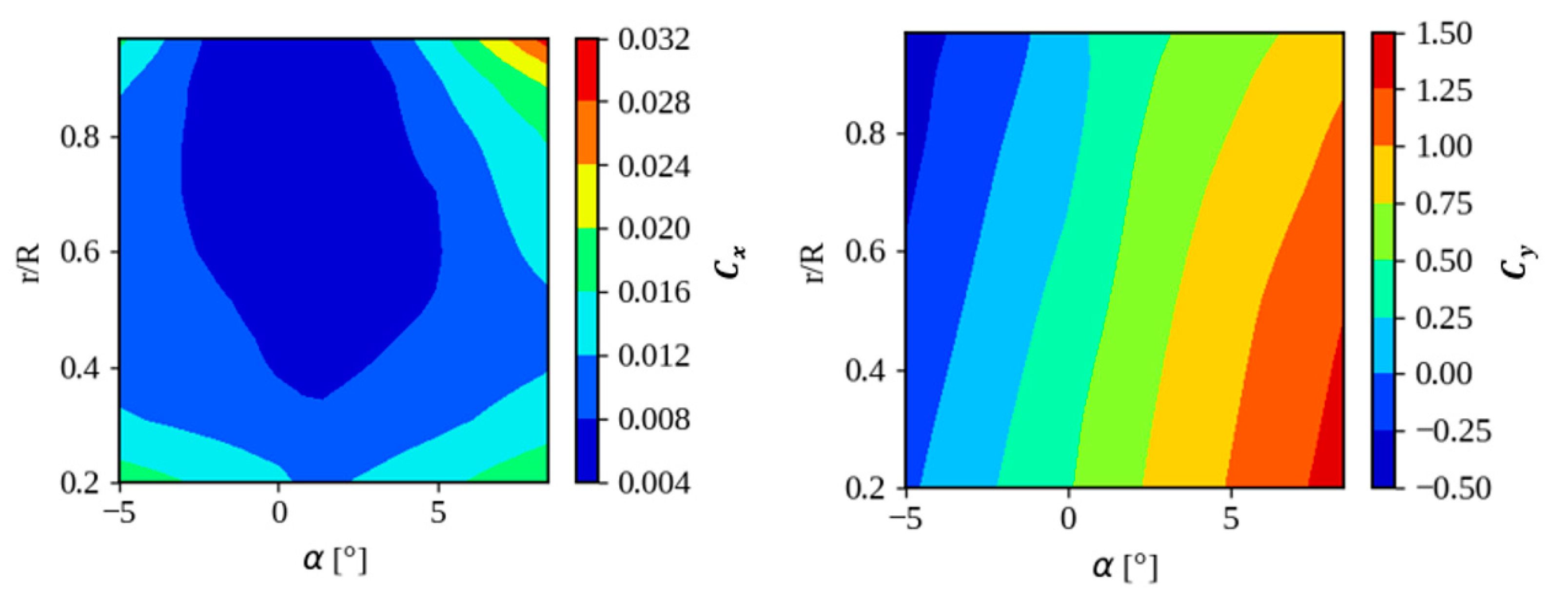
To determine the aerodynamic characteristics of the propeller and reduce the number of calculations, interpolation of the profile data was performed over a smaller number of sections, in which the characteristics of the angle of attack were calculated considering the local Reynolds and Mach numbers (see Figure 4).

A study was conducted out on the required number of sections, which showed that the use of 15 sections to calculate the aerodynamics of the profile and 75 sections to integrate thrust and moment allows one to quickly obtain accurate values of the propeller characteristics (Figure 5).

2.7. Isolate Section Method Validation

The proposed method of propeller calculation was carried out by comparing it with the experimental data of the NACA 5868–9 propeller (experimental results, geometric and kinematic characteristics of the propeller are given in [45]), as well as by comparison with the results of numerical mathematical modeling by solving the Navier–Stokes equations in ANSYS CFX 18.2 software using the shear stress transport turbulence model. The propeller diameter is 3.15 m. The problem statement and the dimensions of the static and rotational domains are shown in Figure 6. The configuration and dimensions of the domain are based on those shown in [48]. The stator mesh has 2,618,015 tetrahedral elements, and the rotor mesh has 11,130,389 elements (tetrahedra and pyramids). The minimum element sizes were 150 mm for the stationary domain, 15 mm for the rotating domain, 4.0 mm on the propeller wall. The first boundary layer thickness was 0.05 mm. In the CFX calculation, the propeller was modeled together with the nacelle, matching the geometry to the experimental conditions. The free wind speed is 170 km/h, with rotational speeds from 800 rpm to 2500 rpm. Validation was performed for two cases of propeller geometry, with blade angles of φ_0.75 = 25° and φ_0.75 = 35°. The values of the mean residuals for all equations do not exceed 10⁻³. The velocity field and pressure distribution are shown in Figure 7. The comparison results in terms of thrust coefficient and power from the advanced ratio are shown in Figure 8.

2.8. Optimization Algorithm

The optimization algorithm used to solve the task is based on the Differential Evolution (DE) algorithm. The proposed algorithm contemplates the use of self-adaptive schemes of evolutionary operators, methods of Population Size Reduction (PSR), sampling techniques for the selection of individuals from the initial population, and stopping conditions that adapt to the needs of the optimization process. In addition, the developed algorithm contemplates the use of parallel computing strategies to accelerate the calculation of the values of the objective function.

Differential evolution is a stochastic, population-based algorithm developed for real-valued function optimization problems. It operates by having a population of individuals (x vector) that move around in the search space by recombining through crossover and mutation with other existing individuals in the population. Through a selection process, a newly generated individual is accepted as part of the population if the new individual x is an improvement; otherwise, it is discarded. This iteration process is repeated to find a vector x that optimizes a function f(x) [49]. As with other evolutionary algorithms, the search performance of differential evolution algorithms depends on the control parameter settings. A standard differential evolution has three main control parameters: population size, scaling factor F, and crossover factor CR. However, it is well-known that the optimal settings of these parameters are problem dependent. Therefore, when applying differential evolution to a real-world problem, it is often necessary to tune the control parameters to obtain the desired results. In practical cases, many researchers suggest the use of self-adaptive schemes to adjust online control parameters during the search process. A variant of differential evolution that applies this type of scheme is the success history-based adaptation for differential evolution (SHADE) [50]. In previous works by the authors of this article, the good performance of the SHADE algorithm for the optimization of aerodynamic bodies such as wings has been corroborated [51].

In SHADE, the mutation factor F ∈ [0, 1] controls the magnitude of the differential mutation operator and CR ∈ [0, 1] is the crossover factor. In the beginning, the contents of MCR, k, MF, k (k = 1, …, H) are all initialized to 0.5. In each generation g, the control parameters CRi and Fi used by each individual xi are generated by randomly selecting an index ri from [1, H], and then applying the formulas below:

$${\mathrm{C}\mathrm{R}}_{\mathrm{i}}=\left\{\begin{array}{cc}0& \mathrm{i}\mathrm{f}{\mathrm{M}}_{\mathrm{C}\mathrm{R},\mathrm{r}\mathrm{i}}=-1\\ {\mathrm{r}\mathrm{a}\mathrm{n}\mathrm{d}\mathrm{n}}_{\mathrm{i}}\left({\mathrm{M}}_{\mathrm{C}\mathrm{R},\mathrm{r}\mathrm{i}},0.1\right)& \mathrm{o}\mathrm{t}\mathrm{h}\mathrm{e}\mathrm{r}\mathrm{w}\mathrm{i}\mathrm{s}\mathrm{e}\end{array}\right.$$

(43)

$${\mathrm{F}}_{\mathrm{i}}={\mathrm{r}\mathrm{a}\mathrm{n}\mathrm{d}\mathrm{c}}_{\mathrm{i}}\left({\mathrm{M}}_{\mathrm{F},\mathrm{r}\mathrm{i}},0.1\right)$$

(44)

Here, randn_i(M, 0.1), randc_i(M, 0.1) are values selected randomly from normal and Cauchy distributions with mean M and variance 0.1. In case a value for CR_i outside of [0, 1] is generated, it is replaced by the limit value (0 or 1) closest to the generated value. When F_i > 1, F_i is truncated to 1, and when F_i ≤ 0, Equation (44) is repeatedly applied to try to generate a valid value. In Equation (43), if M_CR,ri has been assigned the “terminal value” −1, CR_i is set to 0.

The mutation strategy used by SHADE current-to-pbest/1 is a variant of the current-to-best/1 strategy where the greediness is adjustable using a parameter p.

$${\mathrm{v}}_{\mathrm{i},\mathrm{g}}={\mathrm{x}}_{\mathrm{i},\mathrm{g}}+{\mathrm{F}}_{\mathrm{i}}\left({\mathrm{x}}_{\mathrm{p}\mathrm{b}\mathrm{e}\mathrm{s}\mathrm{t},\mathrm{g}}-{\mathrm{x}}_{\mathrm{i},\mathrm{g}}\right)+{\mathrm{F}}_{\mathrm{i}}\left({\mathrm{x}}_{\mathrm{r}1,\mathrm{g}}-{\mathrm{x}}_{\mathrm{r}2,\mathrm{g}}\right)$$

(45)

The individual x_pbest,g is randomly selected from the top p·NP members in the g-th generation (p ∈ [0, 1]). F_i is the F parameter used by individual x_i. The greediness of current-to-pbest/1 depends on the control parameter p to balance exploitation and exploration (small p behaves more greedily).

SHADE uses binary crossover strategy,

$${\mathrm{u}}_{\mathrm{j},\mathrm{i},\mathrm{g}}=\left\{\begin{array}{cc}{\mathrm{v}}_{\mathrm{j},\mathrm{i},\mathrm{g}}& \mathrm{i}\mathrm{f}\mathrm{r}\mathrm{a}\mathrm{n}\mathrm{d}\left(\mathrm{0,1}\right)\le {\mathrm{C}\mathrm{R}}_{\mathrm{i}}\\ {\mathrm{x}}_{\mathrm{j},\mathrm{i},\mathrm{g}}& \mathrm{o}\mathrm{t}\mathrm{h}\mathrm{e}\mathrm{r}\mathrm{w}\mathrm{i}\mathrm{s}\mathrm{e}\end{array}\right.$$

(46)

Perform selection between the trial vector (u_i,g) and target vector (x_i,g) using a greedy selection criterion,

$${\mathrm{x}}_{\mathrm{i},\mathrm{g}+1}=\left\{\begin{array}{cc}{\mathrm{u}}_{\mathrm{i},\mathrm{g}}& \mathrm{i}\mathrm{f}\mathrm{f}\left({\mathrm{u}}_{\mathrm{i},\mathrm{g}}\right)\le \mathrm{f}\left({\mathrm{x}}_{\mathrm{i},\mathrm{g}}\right)\\ {\mathrm{x}}_{\mathrm{i},\mathrm{g}}& \mathrm{o}\mathrm{t}\mathrm{h}\mathrm{e}\mathrm{r}\mathrm{w}\mathrm{i}\mathrm{s}\mathrm{e}\end{array}\right.$$

(47)

SHADE uses a historical memory M_CR, M_F which stores a set of CR, F values that have performed well in the past, and generates new CR, F pairs by directly sampling the parameter space close to one of these stored pairs.

In Algorithm 3, index k determines the position in memory to be updated. In generation g, the k-element in the memory is updated. At the beginning of the search, k is initialized to 1. k is incremented whenever a new element is inserted into the history. If k > H, k is set to 1. In the updated algorithm 1, note that when all individuals in generation g fail to generate a trial vector that is better than the parent, i.e., S_CR = S_F = ∅, the memory is not updated. The weighted Lehmer mean mean_WL(S) is computed using the following formula:

$${\mathrm{m}\mathrm{e}\mathrm{a}\mathrm{n}}_{\mathrm{W}\mathrm{L}}\left(\mathrm{S}\right)=\frac{{\sum }_{\mathrm{m}=1}^{\left|\mathrm{S}\right|}{\mathrm{w}}_{\mathrm{m}}{\mathrm{S}}_{\mathrm{m}}^2}{{\sum }_{\mathrm{m}=1}^{\left|\mathrm{S}\right|}{\mathrm{w}}_{\mathrm{m}}{\mathrm{S}}_{\mathrm{m}}}$$

(48)

$${\mathrm{w}}_{\mathrm{m}}=\frac{\mathsf{\Delta }{\mathrm{f}}_{\mathrm{m}}}{{\sum }_{\mathrm{l}=1}^{\left|\mathrm{S}\right|}{\mathsf{\Delta }\mathrm{f}}_{\mathrm{l}}}$$

(49)

$${\mathsf{\Delta }\mathrm{f}}_{\mathrm{m}}=\left|\mathrm{f}\left({\mathrm{u}}_{\mathrm{m},\mathrm{g}}\right)-\mathrm{f}\left({\mathrm{x}}_{\mathrm{m},\mathrm{g}}\right)\right|$$

(50)

Algorithm 3: Memory update algorithm in SHADE
	Inputs: SCR, SF, MCR,k,g, MF,k,g, k, H
	Outputs: MCR,k,g+1, MF,k,g+1, k
1	if SCR ≠ ∅ and SF ≠ ∅ then
2	if MCR,k,g = −1 or max(SCR) = 0 then
3	MCR,k,g+1 = −1;
4	else
5	MCR,k,g+1 = meanWL(SCR);
6	MF,k,g+1 = meanWL(SF);
7	k++;
8	if k > H then
9	k = 1;
10	else
11	MCR,k,g+1 = MCR,k,g;
12	MF,k,g+1 = MF,k,g;
13	return Outputs

The amount of fitness improvement ∆f_m is used to influence the parameter adaptation (S refers to either S_CR or S_F). As M_CR is updated, if M_CR,k,g = −1 or max(S_CR) = 0 (i.e., all elements of S_CR are 0), M_CR,k,g+1 is set to −1. Thus, if M_CR is assigned the terminal value −1, then M_CR will remain fixed at −1 until the end of the search. This has the effect of locking CR_i to 0 until the end of the search, causing the algorithm to enforce a “change-one-parameter-at-a-time” policy, which tends to slow down convergence, and is effective on multimodal problems.

The SHADE algorithm works well in conjunction with the PSR methods. To develop this optimization algorithm, we decided to incorporate the continuous adaptive population reduction (CAPR) method. The CAPR method gradually reduces the population size according to the change in the gradient of the fitness value [52].

$${\mathrm{N}\mathrm{P}}_{\mathrm{g}+1}=\left\{\begin{array}{cc}\sqrt[\mathsf{\gamma }]{{\mathsf{\Delta }}_{\mathrm{g}}/{\mathsf{\Delta }}_{\mathrm{g}-1}}& 0<{\mathsf{\Delta }}_{\mathrm{g}}/{\mathsf{\Delta }}_{\mathrm{g}-1}<1\\ {\mathrm{N}\mathrm{P}}_{\mathrm{g}}& \mathrm{o}\mathrm{t}\mathrm{h}\mathrm{e}\mathrm{r}\mathrm{w}\mathrm{i}\mathrm{s}\mathrm{e}\end{array}\right.$$

(51)

$${\mathrm{N}\mathrm{P}}_{\mathrm{g}+1}=\left\{\begin{array}{cc}{\mathrm{N}\mathrm{P}}_{\mathrm{g}+1}& {\mathrm{N}\mathrm{P}}_{\mathrm{g}+1}>{\mathrm{N}\mathrm{P}}_{\mathrm{m}\mathrm{i}\mathrm{n}}\\ {\mathrm{N}\mathrm{P}}_{\mathrm{m}\mathrm{i}\mathrm{n}}& {\mathrm{N}\mathrm{P}}_{\mathrm{g}+1}\le {\mathrm{N}\mathrm{P}}_{\mathrm{m}\mathrm{i}\mathrm{n}}\end{array}\right.$$

(52)

where

$${\mathsf{\Delta }}_{\mathrm{g}}=\frac{{\mathrm{f}}_{\mathrm{a}\mathrm{v}\mathrm{g}}\left({\mathrm{x}}_{\mathrm{g}}\right)-{\mathrm{f}}_{\mathrm{a}\mathrm{v}\mathrm{g}}\left({\mathrm{x}}_{\mathrm{g}-1}\right)}{{\mathrm{f}}_{\mathrm{a}\mathrm{v}\mathrm{g}}\left({\mathrm{x}}_{\mathrm{g}}\right)},{\mathsf{\Delta }}_{\mathrm{g}-1}=\frac{{\mathrm{f}}_{\mathrm{a}\mathrm{v}\mathrm{g}}\left({\mathrm{x}}_{\mathrm{g}-1}\right)-{\mathrm{f}}_{\mathrm{a}\mathrm{v}\mathrm{g}}\left({\mathrm{x}}_{\mathrm{g}-2}\right)}{{\mathrm{f}}_{\mathrm{a}\mathrm{v}\mathrm{g}}\left({\mathrm{x}}_{\mathrm{g}-1}\right)}$$

(53)

In the third generation and in subsequent generations, the evaluated function values of all vectors in the population are averaged to be ${\mathrm{f}}_{\mathrm{a}\mathrm{v}\mathrm{g}}\left({\mathrm{x}}_{\mathrm{g}}\right)$. This value, together with that form the previous evaluation generation, is used to calculate the normalized gradient value ${\mathsf{\Delta }}_{\mathrm{g}}$. ${\mathsf{\Delta }}_{\mathrm{g}-1}$ is calculated in a similar fashion using the previous average function evaluation value, ${\mathrm{f}}_{\mathrm{a}\mathrm{v}\mathrm{g}}\left({\mathrm{x}}_{\mathrm{g}-1}\right)$, and the one before the previous ${\mathrm{f}}_{\mathrm{a}\mathrm{v}\mathrm{g}}\left({\mathrm{x}}_{\mathrm{g}-2}\right)$. If the ratio ${\mathsf{\Delta }}_{\mathrm{g}}$/${\mathsf{\Delta }}_{\mathrm{g}-1}$ is within the range of [0, 1], then NP is reduced by a fraction equal to the γ-th root of the ratio ${\mathsf{\Delta }}_{\mathrm{g}}$/${\mathsf{\Delta }}_{\mathrm{g}-1}$. The reason for taking root of the ratio is to slow down the population size reduction rate.

Another criterion to consider when increasing the performance of algorithms based on differential evolution is the generation of the initial population. It has been shown that a population, whose individuals are best distributed throughout the entire design space, has a greater chance of finding a global optimum, in addition to reducing the search time. The LHS design is a statistical method for generating a quasi-random sampling distribution. It is one of the most popular sampling techniques used in computer experiments because of its simplicity and projection properties with high-dimensional problems. The LHS is built as follows: each dimensional space, representing a variable, is cut into n sections, where n is the number of sampling points, and only one point is placed in each section [53].

For real-case optimization processes, it is common to use two types of stopping criteria. The following two types of stopping criteria were considered for this algorithm [54]:

• Exhaustion-based criteria: due to limited computational resources, the optimization run might be terminated after a certain number of objective function evaluations or CPU time. Typically, a maximum number of generations or number of objective function evaluations is used in combination with every stopping criterion to prevent the algorithm from running forever if a criterion cannot stop the run.
• Distribution-based criteria: for differential evolution algorithms, all individuals eventually converge to the optimum. Therefore, it can be concluded that convergence occurs when individuals are close to each other. Because it is assumed that the optimum is not known for the reference criterion, the distances between the population members are examined. This type of criterion can be applied to the design space or objective space.

One of the main disadvantages of evolutionary algorithms is that they need to evaluate multiple vectors to find the global optimum, which implies calculating the values of the objective function many times. One way to speed up the calculation process is to use parallel computing strategies. The strategy that was proposed to be used is Lightweight Pipelining (LP) [55]. The pipelining process provides an easy approach for downloading and using the models on demand. It helps in parallelization, which means that different jobs can be run in parallel. It also reduces redundancy and helps to inspect and debug the data flow in the model. Some features that pipeline provides are on-demand computing, tracking of data and computation, and inspection of data flow.

OpenVINT is the union and adaptation of each of the aforementioned algorithms and methods to achieve the objective of the optimization process mentioned at the beginning of this work. Coding of this algorithm was performed mainly on Python 3 in a GNU/LINUX environment.

3. Results

3.1. Case Studies

To evaluate the performance of the OpenVINT algorithm, two cases were performed:

• case 1—obtain the optimal design of a propeller used for an engine of a fixed-wing aircraft, considering a free flow velocity of 25 m/s and a minimum required thrust is 7.5 N;
• case 2—obtain the optimal design of a propeller used in a helicopter, considering a free flow velocity of 2 m/s and a minimum thrust required is 6.5 N.

In both cases, the following physical properties of the air flow were used: ρ, 1.225 kg/m³; ν, 0.000014607 m²/s; and a, 340.294 m/s. The intervals of the design variables implemented in each of the tests are shown in

Table 1. Intervals of the design variables.

Parameter	Interval		Variable	Interval
	Case 1	Case 2		Case 1	Case 2
(c/d)r	[0.03, 0.10]	[0.05, 0.07]	xtt	[0.30, 0.40]	[0.30, 0.40]
(c/d)m	[0.03, 0.10]	[0.08, 0.13]	$\overline{\mathrm{r}}$xtm	[0.30, 0.80]	[0.20, 0.50]
(c/d)t	[0.01, 0.02]	[0.01, 0.03]	ycr	[0.01, 0.05]	[0.05, 0.08]
$\overline{\mathrm{r}}$cm	[0.35, 0.60]	[0.20, 0.50]	ycm	[0.01, 0.05]	[0.05, 0.08]
αr [°]	[−7, 7]	[0, 5]	yct	[0.005, 0.05]	[0.05, 0.08]
αm [°]	[−5, 7]	[0, 5]	$\overline{\mathrm{r}}$ycm	[0.30, 0.80]	[0.20, 0.50]
αt [°]	[−5, 7]	[0, 5]	xcr	[0.30, 0.40]	[0.30, 0.40]
$\overline{\mathrm{r}}$αm	[0.25, 0.75]	[0.20, 0.50]	xcm	[0.30, 0.45]	[0.30, 0.40]
ytr	[0.12, 0.20]	[0.10, 0.20]	xct	[0.30, 0.45]	[0.30, 0.40]
ytm	[0.12, 0.16]	[0.08, 0.10]	$\overline{\mathrm{r}}$xcm	[0.30, 0.80]	[0.20, 0.50]
ytt	[0.10, 0.12]	[0.08, 0.10]	nm [rev/min]	[5 × 103, 10 × 103]	[5 × 103, 10 × 103]
$\overline{\mathrm{r}}$ytm	[0.30, 0.80]	[0.20, 0.50]	B	[2, 4]	[2, 3]
xtr	[0.30, 0.40]	[0.30, 0.40]	d [m]	[0.3, 0.3]	[0.254, 0.254]
xtm	[0.30, 0.45]	[0.30, 0.40]

.

For both optimization cases the following parameters of the optimization algorithm were taken:

• in real optimization problems it is considered to use at least 50 individuals in the initial population [56], and as a minimum population 10 individuals were considered;
• the stop conditions contemplated were a maximum number of evaluated generations of 200, and an ε value of 1 W to fulfill the condition indicated in line 45 of Algorithm 4;
• a γ factor of 50 was used in (51);
• finally, an initial U* value of 350 W was considered.

All the tests were performed on a PC whose characteristics are as follows:

• operative system, Ubuntu 22.04.3 LTS;
• processor, 13th Gen Intel^® Core^TM i5-13400Fx12;
• RAM memory, 64 GB;

Algorithm 4: OpenVINT algorithm
	Inputs: d, V∞, ρ, ν, a, Tmin, $\overline{\mathrm{r}}$, NS, [Xmin, Xmax], G, NP, NPmin, ε, U*, γ, H, p
	Outputs: xopt, L(xopt)
	//Initialization phase
1	g = 1;
2	Initialize of metrics;
3	Initialize population Pg with LHS;
	//Parallelized loop by joblib
4	for i = 1 to NP do
5	Apply Algorithm 1 for xi,g;
	//Parallelized loop by joblib
6	for i = 1 to NP do
7	Get T(xi,g), W(xi,g), ηd(xi,g), ηs(xi,g) with Algorithm 2;
8	Get ψ(xg) with (2) and L(xg) with (1);
9	Update U*;
10	Save Lavg(xg);
11	Save data of generation g;
12	Set all values in MCR, MF to 0.5;
13	Archive A = ∅;
14	k = 1;
	//Main loop
15	for g = 2 to G do
16	SCR = ∅, SF = ∅;
17	for i = 1 to NP do
18	ri = select from [1, H] randomly;
19	Get CRi,g with (43);
20	Get Fi,g with (44);
21	Get mutation vector vi,g with (45);
22	Get trial vector ui,g with (46);
	//Parallelized loop by joblib
23	for i = 1 to NP do
24	Apply Algorithm 1 with ui,g;
	//Parallelized loop by joblib
25	for i = 1 to NP do
26	Get T(ui,g), W(ui,g), ηd(ui,g), ηs(ui,g) with Algorithm 2;
27	Get ψ(ug) with (2) and L(ug) with (1);
28	Update U*;
29	for i = 1 to NP do
30	if L(ui,g) ≤ L(xi,g) then
31	xi,g+1 = ui,g;
32	xi,g→A;
33	CRi,g→SCR, Fi,g→SF;
34	else
35	xi,g+1 = xi,g;
36	Update memories MCR and MF with Algorithm 3;
37	Save Lavg(xg+1);
38	if g ≥ 3 then
39	Get Δg and Δg−1 with (53);
40	Get NPg+1 with (51);
41	if NPg+1 < NPmin then
42	Apply (52);
43	(NPg − NPg+1)-th worst vectors → A;
44	Save data of generation g+1;
45	if |Lavg(xg+1) − Lopt(xg+1)| ≤ε then
46	break;
47	k++;
48	Print metrics plots;
49	Output
50	Drawing the optimal propeller in point clouds;

3.2. Optimization Results

For case 1, the following parameters of the optimization algorithm were taken:

• 6 tests were performed, 3 of them were with an initial population of 50 vectors and the other 3 with an initial population of 100 vectors;
• a minimum population of 10 vectors was considered in all tests;
• the stop conditions contemplated were a maximum number of evaluated generations of 200, and an ε value of 1 W to fulfill the condition indicated in line 48 of algorithm 4;
• a γ factor of 50 was used in (51);
• finally, an initial U* value of 350 W was considered.

Figure 9 shows the convergence graphs of the metrics used to evaluate the propeller optimization process for case 1.

Table 2. Results obtained from case 1.

Parameter	NP = 50					NP = 100
	Test 1	Test 2	Test 3	Mean	CV, [%]	Test 4	Test 5	Test 6	Mean	CV, [%]
(c/d)r	0.043	0.082	0.094	0.073	29.45	0.035	0.038	0.043	0.039	8.04
(c/d)m	0.100	0.094	0.088	0.094	5.21	0.085	0.087	0.100	0.091	7.40
(c/d)t	0.012	0.015	0.018	0.015	15.33	0.020	0.020	0.019	0.020	3.42
$\overline{\mathrm{r}}$cm	0.509	0.400	0.600	0.503	16.29	0.551	0.587	0.522	0.553	4.82
αr [°]	0.243	−0.784	6.288	1.916	162.84	4.214	−7.000	6.245	1.153	505.15
αm [°]	6.144	5.278	4.307	5.243	14.31	6.956	6.081	5.609	6.216	8.98
αt [°]	4.823	6.973	2.324	4.707	40.36	4.632	4.770	5.217	4.873	5.12
$\overline{\mathrm{r}}$αm	0.253	0.251	0.250	0.251	0.60	0.253	0.286	0.605	0.381	41.62
ytr	0.070	0.060	0.066	0.066	6.41	0.060	0.061	0.061	0.061	0.75
ytm	0.060	0.061	0.061	0.061	0.66	0.060	0.060	0.060	0.060	0.00
ytt	0.059	0.060	0.054	0.057	3.99	0.053	0.060	0.051	0.055	6.71
$\overline{\mathrm{r}}$ytm	0.745	0.300	0.300	0.448	46.74	0.598	0.530	0.364	0.497	19.73
xtr	0.327	0.300	0.309	0.312	3.52	0.333	0.320	0.308	0.320	3.21
xtm	0.329	0.335	0.300	0.321	4.73	0.332	0.336	0.315	0.328	2.73
xtt	0.330	0.315	0.306	0.317	3.15	0.339	0.384	0.345	0.356	5.65
$\overline{\mathrm{r}}$xtm	0.787	0.722	0.300	0.603	35.75	0.300	0.300	0.357	0.319	8.35
ycr	0.050	0.010	0.029	0.030	54.70	0.026	0.047	0.011	0.028	52.36
ycm	0.010	0.011	0.014	0.012	15.13	0.010	0.010	0.010	0.010	0.00
yct	0.005	0.016	0.028	0.016	57.93	0.006	0.005	0.006	0.006	8.31
$\overline{\mathrm{r}}$ycm	0.358	0.459	0.652	0.490	24.90	0.483	0.358	0.712	0.518	28.33
xcr	0.338	0.399	0.331	0.356	8.65	0.398	0.395	0.364	0.386	3.95
xcm	0.443	0.443	0.306	0.397	16.28	0.352	0.386	0.387	0.37	4.33
xct	0.361	0.441	0.310	0.370	14.59	0.399	0.367	0.422	0.396	5.77
$\overline{\mathrm{r}}$xcm	0.692	0.407	0.778	0.626	25.32	0.643	0.800	0.505	0.649	18.58
nm [rev/min]	6156	6238	6765	6386	4.22	6281	6312	5993	6195	2.32
B	2	2	2	2	0	2	2	2	2	0
d [m]	0.300	0.300	0.300	0.300	0	0.300	0.300	0.300	0.300	0
W [W]	226.8	225.7	228.1	226.9	0.44	226.0	226.7	225.7	226.1	0.18
T [N]	7.513	7.504	7.506	7.508	0.05	7.501	7.512	7.512	7.509	0.07
ηd	0.828	0.831	0.823	0.827	0.41	0.830	0.828	0.832	0.830	0.18
Computation time [s]	3897	4728	4417	4347	7.89	9987	9526	10,703	10,072	4.81

shows the values of the optimal design vector as well as the optimal values of the required power output, thrust provided, and the dynamic efficiency of the propeller. In addition, the average values, and the coefficient of variation (CV) for each parameter are shown, which allows evaluation of the homogeneity of the data.

The geometric differences between each of the blades obtained for case 1 can be visualized in Figure 10 and Figure 11.

For case 2 the following parameters of the optimization algorithm were taken:

• A total of 3 tests were performed, with an initial population of 50 vectors and a minimum population of 10 vectors;
• the stop conditions contemplated were a maximum number of evaluated generations of 200, and an ε value of 1 W to fulfill the condition indicated in line 48 of algorithm 4;
• a γ factor of 50 was used in (51);
• finally, an initial U* value of 350 W was considered.

Figure 12 shows the convergence graphs of the metrics used to evaluate the propeller optimization process. The final values of the optimization are shown in more detail in

Table 3. Results obtained from the case 2.

Parameter	Test 1	Test 2	Test 3	Mean	CV, [%]
(c/d)r	0.063	0.070	0.055	0.063	9.78
(c/d)m	0.130	0.120	0.125	0.125	3.27
(c/d)t	0.030	0.028	0.030	0.029	3.21
$\overline{\mathrm{r}}$cm	0.456	0.500	0.478	0.478	3.76
αr [°]	0.000	0.718	3.579	1.432	107.93
αm [°]	4.625	2.254	3.772	3.550	27.62
αt [°]	1.619	1.193	3.734	2.182	50.92
$\overline{\mathrm{r}}$αm	0.435	0.327	0.500	0.421	16.96
ytr	0.063	0.073	0.093	0.076	16.34
ytm	0.042	0.040	0.040	0.041	2.31
ytt	0.046	0.043	0.042	0.044	3.89
$\overline{\mathrm{r}}$ytm	0.251	0.200	0.208	0.220	10.19
xtr	0.300	0.382	0.356	0.346	9.89
xtm	0.331	0.301	0.329	0.320	4.28
xtt	0.361	0.300	0.390	0.350	10.71
$\overline{\mathrm{r}}$xtm	0.497	0.200	0.248	0.315	41.33
ycr	0.064	0.062	0.069	0.065	4.53
ycm	0.051	0.051	0.052	0.051	0.92
yct	0.050	0.053	0.051	0.051	2.43
$\overline{\mathrm{r}}$ycm	0.272	0.226	0.222	0.240	9.45
xcr	0.386	0.398	0.334	0.372	7.45
xcm	0.300	0.302	0.300	0.301	0.31
xct	0.323	0.301	0.301	0.308	3.36
$\overline{\mathrm{r}}$xcm	0.263	0.249	0.209	0.240	9.52
nm [rev/min]	6720	7662	6705	7209	6.37
B	2	2	2	2	0.00
d [m]	0.254	0.254	0.254	0.254	0.00
W [W]	72.56	72.17	72.24	72.32	0.23
T [N]	6.505	6.516	6.505	6.509	0.08
ηs	0.649	0.654	0.652	0.652	0.32
Computation time [s]	3333	3743	3227	3434	6.48

.

Graphically, the differences between the blades obtained in each of the tests can be observed in Figure 13 and Figure 14.

3.3. Experimental Validation

To verify the results obtained in the optimization process, one of the propellers obtained in the tests performed for case 2 (the propeller obtained in test 3) was selected. The propeller was manufactured by contact molding continuous carbon fibers using epoxy thermosetting binder in a closed mold. The mold was fabricated using a CNC milling machine from the geometry obtained in test 3 (Figure 15). The outer layers and the spars passing through the sleeve comprise unidirectional fibers, and the inner two layers are stacked from plain fabric with fiber orientation ±45°.

The proposed experimental setup allows the monitoring of the angular velocity, thrust, and torque of the propeller. The angular velocity of the propeller was monitored using two different methods: measurement from the electric motor with a PWM frequency meter and measurement from the propeller with a laser photo tachometer. The thrust and torque of the propeller are measured using strain gauges at the base of the motor. The power requirement of the propeller was calculated as the product of torque and angular velocity (see Figure 16) [57].

A comparison was made of the dependences of thrust on the required power for two propellers—designed (test 2, case 3) and commercial DJI 10 × 4.5′′ propeller (Figure 17). Seven experimental tests (T1…T7) were carried out for each propeller, varying in rotational speed (Figure 18). Each test consists of from 6 to 8 measurements—a total of 46 measurements for designed propeller and 49 measurements for DJI propeller. The dependences of thrust on required power for each test were interpolated by smooth univariable spline of 3 degrees and then lines of average values and scatter equal to the standard deviation are plotted (Figure 19).

Comparison of calculated by ISM and experimental data for the designed propeller (Figure 19a) showed that for the main propeller regimes (trust more than 2N) the difference does not exceed 3.5%. A comparison between the designed propeller and a commercially available propeller (DJI 10 × 4.5′′ propeller) is shown in Figure 19b. The proposed algorithm demonstrates that it can design a propeller that provides a higher thrust (from 10 to 15%) with the same power requirement as commercial propellers in main operating mode.

4. Discussion

In the results of the tests carried out, presented in Table 2 and Table 3, the following points could be observed:

• for the optimization of a helicopter propeller, it is sufficient to use an initial population of 50 vectors to obtain similar results (CV values less than 30%);
• to optimize a tractor propeller, it was necessary to use an initial population of 100 vectors to improve the search for a global optimal;
• in both cases, there is a greater variation in the parameters that describe the geometry of the blade root, whereas in the parameters that describe the rest of the blade geometry, the results were more homogeneous.

Figure 9 and Figure 12 illustrate that in the most representative blade section (in 75% of the blade length), practically similar cross-sectional (airfoil) geometries are obtained. Similar aerodynamic behavior implies that similar values of thrust provided and thrust required are obtained.

When performing the experimental tests with one of the propellers obtained in case 2, it was observed that the aerodynamic characteristics of the propeller obtained with the help of the ISM and XFOIL were comparable to those obtained in the experimental tests, as shown in Figure 19a. These results provide certainty in the calculated values of the objective function for each vector evaluated in the optimization process. While in the comparison that was made with one of the optimized propellers and with a commercial propeller, it was observed that the OpenVINT algorithm provides new propeller options that require less power to achieve a certain thrust.

Regarding the calculation speed of the algorithm, it can be observed that the OpenVINT algorithm provides better performance when optimizing propellers used in helicopters. For this type of propeller, the algorithm requires approximately 1 h of calculation (using a computer as described in Section 3.1), whereas optimizing a tractor propeller for the engine of a fixed-wing aircraft requires approximately 3 h of calculation. Of course, these times can still improve the design space for each type of propeller. This type of analysis is proposed for future studies.

5. Conclusions

The paper presents an algorithm for propeller shape optimization based on isolated section method, similar to BEMT. Using Bezier curves to specify the dependencies of the parameters of thickness, curvature, and positions of the maximum thickness and maximum curvature of the airfoil along the blade span allows the aerodynamic twist of the blade to be varied.

The usage of a cross-section airfoil angle of attack as a function of blade span as design variable adds robustness to the optimization algorithm, protecting from calculation airfoil characteristics at supercritical angles of attack and reduce the number of calculations during the optimization. This makes it possible to reduce the optimization time and increase the accuracy of the optimization solution with geometric models with a large number of design variables and cross-sections used for calculations. Interpolation of the aerodynamic characteristics of sections along the blade span also makes it possible to reduce calculation time. The proposed algorithm allows for obtaining the optimal geometry of the pusher and tractor propellers based on 27 design variables, containing a variable along the blade span airfoil, a nonlinear distribution of twist and chord along the span in three hours of calculation on a personal computer.

In the tests to which OpenVINT optimization algorithm was subjected, it was observed that the parameterization of the proposed propeller geometry is good but still has room for improvement. From the 27 proposed design parameters, the parameters describing the shape of the blade root have little importance in determining the aerodynamic performance of the propeller, which implies that the number of design parameters can be reduced, or the value of these parameters can be refined using multidisciplinary optimization, for example based on stiffness and strength constraints.

The experimental tests validate the calculation method and confirm that the algorithm in general can provide configurations with better aerodynamic performance to the propellers that are available on the market.

References

1. Chen, G.; Ma, D.; Jia, Y.; Xia, X.; He, C. Comprehensive Optimization of the Unmanned Tilt-Wing Cargo Aircraft with Distributed Propulsors. IEEE Access 2020, 8, 137867–137883. [Google Scholar] [CrossRef]
2. Traub, L.W. Considerations in optimal propeller design. J. Aircr. 2021, 58, 8. [Google Scholar] [CrossRef]
3. Betz, A. Introduction to the Theory of Flow Machines; Pergamon Press: Oxford, UK, 1966. [Google Scholar]
4. Betz, A. Schraubenpropeller Mit Geringstem Energieverlust (Screw Propeller with Least Energy Loss); Akademie der Wissenschaften: Gottingen, Germany, 1919; pp. 193–217. [Google Scholar]
5. Adkins, C.N.; Liebeck, R.H. Design of Optimum Propellers. J. Propul. Power. 1994, 10, 676–682. [Google Scholar] [CrossRef]
6. Aleksandrov, V.L. Vozdushnye Vinty; Gosudarstvennoe Izdatel’stvo Oboronnoj Promyshlennosti: Moscow, Russia, 1951; 476p. (In Russian) [Google Scholar]
7. Kümmel, A.; Breitsamter, C. Multi-Disciplinary Framework for Propeller Blade Design. IOP Conf. Ser. Mater. Sci. Eng. 2021, 1024, 012060. [Google Scholar] [CrossRef]
8. Chen, W.; Chiu, K.; Fuge, M.D. Airfoil Design Parameterization and Optimization Using Bézier Generative Adversarial Networks. AIAA J. 2020, 58, 4723–4735. [Google Scholar] [CrossRef]
9. Gur, O.; Rosen, A. Optimization of Propeller Bases Propulsion Systems. J. Aircr. 2009, 46, 95–106. [Google Scholar] [CrossRef]
10. Dorfling, J.; Rokhsaz, K. Constrained and Unconstrained Propeller Blade Optimization. J. Aircr. 2015, 52, 1179–1188. [Google Scholar] [CrossRef]
11. Yu, P.; Peng, J.; Bai, J.; Han, X.; Song, X. Aeroacoustic and Aerodynamic Optimization of Propeller Blades. Chin. J. Aeronaut. 2020, 33, 826–839. [Google Scholar] [CrossRef]
12. Wang, S.; Zhang, S.; Ma, S. An Energy Efficiency Optimization Method for Fixed Pitch Propeller Electric Aircraft Propulsion Systems. IEEE Access 2019, 7, 159986–159993. [Google Scholar] [CrossRef]
13. Bekele, E.G.; Nicklow, J.W. Multi-objective automatic calibration of SWAT using NSGA-II. J. Hydrol. 2007, 341, 165–176. [Google Scholar] [CrossRef]
14. Ma, R.; Zhong, B.W.; Liu, P.Q. Optimization design study of low-Reynolds-number high-lift airfoils for the high-efficiency propeller of low-dynamic vehicles in stratosphere. Sci. China Technol. Sci. 2010, 53, 2792–2807. [Google Scholar] [CrossRef]
15. Slavik, S.; Klesa, J.; Brabec, J. Propeller Selection by Means of Pareto-Optimal Sets Applied to Flight Performance. Aerospace 2020, 7, 21. [Google Scholar] [CrossRef]
16. Fang, B.R. Design of Aircraft Aerodynamic Configuration; Chinese Aviation Industry Press: Beijing, China, 1997; pp. 97–130. [Google Scholar] [CrossRef]
17. Colozza, A. High Altitude Propeller Design and Analysis Overview; NASA/CR 98-208520; Federal Data Systems: Cleveland, OH, USA, 1998. [Google Scholar]
18. Morgado, J.; Abdollahzadeh, M.; Silvestre, M.; Páscoa, J. High Altitude Propeller Design and Analysis. Aerosp. Sci. Technol. 2015, 45, 398–407. [Google Scholar] [CrossRef]
19. Burdett, T.A.; Van Treuren, K.W. A Theoretical and Experimental Comparison of Optimizing Angle of Twist Using BET and BEMT. In Proceedings of the ASME Turbo Expo 2012: Turbine Technical Conference and Exposition. Volume 6: Oil and Gas Applications; Concentrating Solar Power Plants; Steam Turbines; Wind Energy, Copenhagen, Denmark, 11–15 June 2012; pp. 797–809. [Google Scholar] [CrossRef]
20. Oliveira, H.A.; de Matos, J.G.; Ribeiro, L.A.d.S.; Saavedra, O.R.; Vaz, J.R.P. Assessment of Correction Methods Applied to BEMT for Predicting Performance of Horizontal-Axis Wind Turbines. Sustainability 2023, 15, 7021. [Google Scholar] [CrossRef]
21. Goldstein, S. On The Vortex Theory of Screw Propellers. Proc. R. Soc. 1929, 123, 440–465. [Google Scholar] [CrossRef]
22. Zhong, W.; Wang, T.G.; Zhu, W.J.; Shen, W.Z. Evaluation of Tip Loss Corrections to AD/NS Simulations of Wind Turbine Aerodynamic Performance. App. Sci. 2019, 9, 4919. [Google Scholar] [CrossRef]
23. Branlard, E.; Dixon, K.; Gaunaa, M. Vortex Methods to Answer The Need For Improved Understanding And Modelling of Tip-Loss Factors. IET Renew. Power Gener. 2013, 7, 311–320. [Google Scholar] [CrossRef]
24. Elkhchine, Y.; Sriti, M. Tip Loss Factor Effects on Aerodynamic Performances of Horizontal Axis Wind Turbine. Energy Procedia 2017, 118, 136–140. [Google Scholar] [CrossRef]
25. Shaidakov, V.I. Aerodinamika Vinta v kol’ce: Uch Posobie; MAI: Moscow, Russia, 1996; 88p. (In Russian) [Google Scholar]
26. Wald, Q.R. The Aerodynamics of Propellers. Prog. Aerosp. Sci. 2006, 42, 85–128. [Google Scholar] [CrossRef]
27. XFOIL Subsonic Airfoil Development System. Available online: https://web.mit.edu/drela/Public/web/xfoil/ (accessed on 10 January 2024).
28. Munguia, J.; Van Treuren, W. Designing Small Propellers for Optimum Efficiency; Baylor University: Waco, TX, USA, 2019. [Google Scholar]
29. Pierret, S.S.; Van den Braembussche, R.A. Turbomachinery Blade Design Using a Navier-Stokes Solver and Artificial Neural Net-work. J. Turbomach. 1999, 121, 326–332. [Google Scholar] [CrossRef]
30. Segui, M.M.; Castelar, Y.; Botez, R.M. Wing Airfoils Generation Based on a New Parametric Curve for Aerodynamic Optimization Application. In Proceedings of the CASI AERO-2019 Conference, Big Sky, MT, USA, 2–9 March 2019; Canadian Aeronautics and Space Institute: Montreal, QC, Canada, 2019. [Google Scholar]
31. Shikhar Jaiswal, A. Shape Parameterization of Airfoil Shapes Using Bezier Curves. In Innovative Design and Development Practices in Aerospace and Automotive Engineering; Bajpai, R.P., Chandrasekhar, U., Eds.; Lecture Notes in Mechanical Engineering; Springer: Berlin/Heidelberg, Germany, 2017. [Google Scholar] [CrossRef]
32. Alexeev, R.A.; Tishchenko, V.A.; Gribin, V.G.; Gavrilov, I.Y. Turbine Blade Profile Design Method Based on Bezier Curves. J. Phys. Conf. Ser. 2017, 891, 012254. [Google Scholar] [CrossRef]
33. Hao, X.; Zhang, W.; Liu, X.; Liu, J. Aerodynamic and Aeroacoustic Optimization of Wind Turbine Blade by a Genetic Algorithm. In Proceedings of the 46th AIAA Aerospace Sciences Meeting and Exhibit,AIAA 2008-1331, Reno, NV, USA, 7–10 January 2008. [Google Scholar] [CrossRef]
34. Borovkov, A.I.; Voinov, I.B.; Ibraev, D.F. Determination of the Optimal Aerodynamic Shape for a Propeller Blade Based on Parametric Optimization. Russ. Aeronaut. (Iz VUZ) 2021, 64, 173–180. [Google Scholar] [CrossRef]
35. Ayaz Ümütlü, H.C.; Kiral, Z. Airfoil Shape Optimization using Bézier Curve and Genetic Algorithm. Aviation 2022, 26, 32–40. [Google Scholar] [CrossRef]
36. Xin, P.; Dawei, L.; Jixiang, S.; Yonghong, L. Airfoil Aerodynamic Optimization Based on an Improved Genetic Algorithm. In Proceedings of the Fifth International Conference on Intelligent Systems Design and Engineering Applications, Hunan, China, 15–16 June 2014; pp. 133–137. [Google Scholar] [CrossRef]
37. Jiao, J.; Song, B.-F.; Zhang, Y.-G.; Li, Y.-B. Optimal Design and Experiment of Propellers for High Altitude Airship. Proc. Inst. Mech. Eng. Part. G J. Aerosp. Eng. 2017, 232, 1887–1902. [Google Scholar] [CrossRef]
38. Bocii, L.S.; Di Noia, L.P.; Rizzo, R. Optimization of the Energy Storage of Series-Hybrid Propelled Aircraft by means of Integer Differential Evolution. Aerospace 2019, 6, 59. [Google Scholar] [CrossRef]
39. Muratoglu, A.; Tekin, R.; Ertugrul, O.F. Hydrodynamic Optimization of High-Performance Blade Sections for Stall Regulated Hydrokinetic Turbines Using Differential Evolution Algorithm. Ocean Eng. 2021, 220, 108389. [Google Scholar] [CrossRef]
40. Spera, D.A. Models of Lift and Drag Coefficients of Stalled and Unstalled Airfoils in Wind Turbines and Wind Tunnels; Technical Report NASA/CR-2008-215434; GRC: Cleveland, OH, USA, 2008. [Google Scholar]
41. Quijada Pioquinto, J.G.; Kurkin, E.I.; Nazarov, D.V.; Lukyanov, O.E.; Chertykovtseva, V.O. Programma OpenVINT Optimzacii Formy Lopasti Vozdushnogo Vinta [OpenVINT Code for Optimizing the Shape of a Propeller Blade]; RU 2024610972, FIPS: Moscow, Russia, 2024; Available online: https://new.fips.ru/registers-doc-view/fips_servlet?DB=EVM&DocNumber=2024610972&TypeFile=html (accessed on 20 February 2024).
42. Ali, M.M.; Zhu, W.X. A penalty function-based differential evolution algorithm for constrained global optimization. Comput. Optim. Appl. 2013, 54, 707–739. [Google Scholar] [CrossRef]
43. Van To, T.; Ngoc Phien, H. Development of Bezier-based curves. Comput. Ind. 1992, 20, 109–115. [Google Scholar] [CrossRef]
44. Zherejov, V.V.; Kusumov, A.N. Aehrodinamicheskij Raschet Nesushchego Vinta Vertoleta. Uch Posobie Po Kursovomu I Diplomnomu Proektirovaniyu; KGTU: Kazan, Russia, 1997; 28p. (In Russian) [Google Scholar]
45. Kravec, A.S. Kharakteristiki Vozdushnykh Vintov; Uchebnoe Posobie, Gos. Izd. Oboronnoj Promyshlennosti: Moscow, Russia, 1941. (In Russian) [Google Scholar]
46. Derksen, R.W.; Rogalsky, T. Bezier-PARSEC: An Optimized Aerofoil Parameterization for Design. Adv. Eng. Softw. 2010, 41, 923–930. [Google Scholar] [CrossRef]
47. Espinosa Barcenas, O.U.; Quijada Pioquinto, J.G.; Kurkina, E.; Lukyanov, O. Surrogate aerodynamic wing modeling based on a multilayer perceptron. Aerospace 2023, 10, 149. [Google Scholar] [CrossRef]
48. Lin, J.; Yao, H.D.; Wang, C.; Su, Y.; Yang, C. Hydrodynamic performance of a rim-driven thruster improved with gap geometry adjustment. Eng. Appl. Comput. Fluid. Mech. 2023, 17, 2183902. [Google Scholar] [CrossRef]
49. Eltaeib, T.; Mahmood, A. Differential Evolution: A Survey and Analysis. App. Sci. 2018, 8, 1954. [Google Scholar] [CrossRef]
50. Tanabe, R.; Fukunaga, A.S. Improving the search performance of SHADE using linear population size reduction. In Proceedings of the IEEE Congress on Evolutionary Computation (CEC), Beijing, China, 6–11 July 2014; pp. 1200–1207. [Google Scholar] [CrossRef]
51. Espinosa Barcenas, O.U.; Quijada Pioquinto, J.G.; Kurkina, E.; Lukyanov, O. Multidisciplinary analysis and optimization method for conceptually designing of electric flying-wing unmanned aerial vehicles. Drones 2022, 6, 307. [Google Scholar] [CrossRef]
52. Wong, I.; Liu, W.; Ho, C.H.; Ding, X. Continuous adaptive population reduction (CAPR) for differential evolution optimization. SLAS Technol. 2017, 22, 289–305. [Google Scholar] [CrossRef] [PubMed]
53. Iman, R.L. Encyclopedia of Quantitative Risk Analysis and Assessment; John Wiley Sons: Hoboken, NJ, USA, 2008; pp. 408–411. [Google Scholar]
54. Zielinksi, K.; Weitkemper, P.; Laur, R.; Kammeyer, K.D. Examination of Stopping Criteria for Differential Evolution Based on a Power Allocation Problem. Available online: https://api.semanticscholar.org/CorpusID:13358798 (accessed on 2 November 2023).
55. Sharma, H. Lightweight Pipelining in Python. Using Joblib for Storing the Machine Learning Pipeline to a File. Available online: https://towardsdatascience.com/lightweight-pipelining-in-python-1c7a874794f4 (accessed on 2 November 2023).
56. Piotrowski, A.P. Review of differential evolution population size. Swarm Evol. Comput. 2017, 32, 1–24. [Google Scholar] [CrossRef]
57. Lukyanov, O.E.; Espinosa Barcenas, O.U.; Zolotov, D.V. Experimental model of an electric power plant for small UAV’s automatic control systems. In Proceedings of the 2021 International Scientific and Technical Engine Conference, Samara, Russia, 23–25 June 2021. [Google Scholar]
Figure 1. The Bezier curves determine the variation of the design variables.
Computation 12 00052 g001
Figure 2. Airfoil construction using cubic Bezier curves.
Computation 12 00052 g002
Figure 3. Drawing of a blade from Bezier curves and the geometric twist curve.
Computation 12 00052 g003
Figure 4. Aerodynamic coefficients of the CLARK Y profile by different methods.
Computation 12 00052 g004
Figure 5. Calculation and interpolation of aerodynamic characteristics of the profile by propeller span.
Computation 12 00052 g005
Figure 6. NACA 5868-9 propeller calculation in ANSYS CFX, (a) the problem statement, (b) the domain dimensions.
Computation 12 00052 g006
Figure 7. Example of NACA 5868-9 propeller calculation for 1500 rpm and φ0.75 = 25° case, (a) velocity in stationary domain, (b) pressure at propeller wall.
Computation 12 00052 g007
Figure 8. Comparison by thrust coefficient (a) and power coefficient (b).
Computation 12 00052 g008
Figure 9. Convergence of the metrics in the tests corresponding to case 1.
Computation 12 00052 g009
Figure 10. Top view of the propeller blades obtained for case 1.
Computation 12 00052 g010
Figure 11. Examples of the cross-sections of the blades obtained for case 1. The airfoils are normalized with chord of length 1.
Computation 12 00052 g011
Figure 12. Convergence of the metrics in the tests corresponding to case 2.
Computation 12 00052 g012
Figure 13. Top view of the propeller blades obtained for case 2.
Computation 12 00052 g013
Figure 14. Examples of the cross-sections (airfoils) of the blades obtained for case 2. The airfoils are normalized with chord of length 1.
Computation 12 00052 g014
Figure 15. (a) Injection mold for the manufacture of the propellers; (b) manufactured propellers.
Computation 12 00052 g015
Figure 16. Experimental setup.
Computation 12 00052 g016
Figure 17. The designed (a) and commercial (b) propellers installed in the experimental setup.
Computation 12 00052 g017
Figure 18. Experimental data of thrust from required power dependence for propellers: (a) designed, (b) commercial DJI propeller.
Computation 12 00052 g018
Figure 19. Mean measurement values and scatter of propeller thrust from power requirement: (a) comparison for designed propeller between experimental values and numerical test, calculated by ISM, (b) comparison between experimental values for designed and commercial DJI propeller.
Computation 12 00052 g019