1. Introduction
Computational Fluid Dynamics (CFD) is one of the most time-consuming activities in High-Performance Computing (HPC). Recent research shows that heterogeneous architectures, with Graphics Processing Units (GPUs) as massively parallel co-processors to the Central Processing Unit (CPU), can accelerate computation processes in various CFD applications [
1,
2,
3,
4,
5,
6,
7]. Developing a general-purpose CFD software to leverage this powerful hardware is challenging and time-intensive, as evidenced by the cited references. However, the capabilities and limitations of CFD codes applied to turbomachinery problem solving have not been widely explored and thoroughly documented, even though it is a complex task [
8]. Exceptions in this field are relatively few [
9,
10,
11,
12].
Since scalability bottlenecks have been found on massively parallel clusters [
13], recent years have seen the implementation of open-source libraries within the OpenFOAM CFD software developed by [
14] to accelerate computations through GPUs [
15]. Examples of these libraries include Cuda For FOAM Link (cufflink), ofgpu, and speedIT. This implementation has been possible due to hardware architecture. GPUs’ numerous simple cores enhance calculation output and mask memory latency through multithreading [
16], while CPU cores rely on less readily available cache memory for this purpose.
Without modifying the original CFD code and applied as a plug-in, these implementations were intended to improve the memory bandwidth, one of the main restrictions to applying OpenFOAM in HPC [
17]. However, reported issues with memory copies and inconsistent speedups have raised concerns about the appropriateness of hardware investments [
18]. Therefore, GPU-enabled libraries have been updated through RapidCFD [
19], an open-source OpenFOAM 2.3.1 fork able to run almost entire simulations on NVIDIA GPUs [
20].
To address the computational challenges of simulating complex fluid flows in hydraulic turbine draft tubes [
21,
22], this work explores the capabilities of RapidCFD and NVIDIA Tesla GPUs (C1060, M2090, and K40) across three heterogeneous architectures within the OpenFOAM environment. Specifically, we focus on the T-99 3D draft tube benchmark [
23,
24] with different structured grid sizes to evaluate the performance and efficiency of these GPU-powered simulations.
Despite the ongoing trend in HPC clusters towards high-density nodes with approximately 10 cores per node alongside accelerators, e.g., GPUs, FPGAs, Xeon PHI, RISCV, and increased cache levels, the interconnected in clusters exceeding 100,000 nodes, encompassing millions of available cores [
17], solving Turbomachinery CFD problems using multiple GPUs within a single node remains feasible. This approach reduces the need for massive clusters or supercomputers, particularly because some grid sizes fall below 100 million cells [
25,
26,
27,
28] and can be handled effectively by modern single-node heterogeneous configurations. However, achieving a higher resolution through larger grid sizes, as advocated by [
29,
30], would necessitate multi-node configurations, falling outside the scope of this current research.
As computational speed is a highly desirable characteristic in these applications, the determination of the most efficient hardware setup was deemed crucial. Following this, tests were conducted on various combinations of linear solvers, preconditioners, and smoothers available within OpenFOAM. Two set values for the convergence tolerance parameter between time steps were then employed in a series of tests to identify the most suitable option for solving the linear equation system. Subsequently, further computational tests were carried out on different grid sizes to provide an estimation of the required Random Access Memory (RAM), utilizing either one GPU in serial mode or two, three, and four GPUs in parallel configurations. Finally, a comparison of the performance between RapidCFD and cufflink, the available alternative implemented in foam-extend version 4.0, was undertaken.
The results presented in this work offer valuable guidance for selecting the most suitable CUDA-based software application to effectively harness GPU computational power for CFD analysis.
2. Methodology
This section details the three massively heterogeneous architectures using NVIDIA Tesla GPUs C1060, M2090, and K40, followed by the key features of the T-99 draft tube benchmark and numerical setup, and concludes with an overview of available linear solvers, preconditioners, and smoothers in OpenFOAM.
2.1. Hardware Architecture
Table 1 summarizes the main features of the heterogeneous architectures used in this work. All three workstations, WSPAC, WSGAL, and WSMOL, respectively, are dual CPUs platforms with four, six, and eight cores, the last two with multi-threading capabilities.
Despite WSPAC and WSMOL offering commercially available pre-configured options, WSGAL presents a non-commercial alternative for assembling custom heterogeneous architectures. These configurations remain relevant in the current hardware landscape, even with ongoing trends towards high-density nodes with accelerators [
31]. While GPUs exhibit slower memory and processing frequency compared to CPUs, their design philosophies differ significantly. CPUs prioritize rapid execution of single-thread operations, capably handling a few tens of operations concurrently. In contrast, GPUs optimize for parallel execution of thousands of threads, effectively mitigating their slower individual performance through sheer throughput [
32]. This contrast is reflected in peak performance: high-end CPUs reach around 50–60 GFLOPS, while modern GPUs exceed 500 GFLOPS [
31].
2.2. T-99 Draft Tube Benchmark and Numerical Setup
Located after the runner in a hydraulic turbine, the draft tube is tasked with converting the kinetic energy of the fluid entering it into pressure energy, minimizing losses as much as possible. The numerical model of the Hölleforsen Kaplan draft tube 1:11, previously employed in three European Research Community on Flow Turbulence and Combustion (ERCOFTAC) workshops [
33,
34,
35,
36], was studied.
Figure 1 presents the computational model of the turbine T-99, equipped with a hexahedral structured grid utilized for the computations.
The computational domains were divided into a grid of interconnected cells and solved with double precision and the Semi-Implicit Method for Pressure-Linked Equations (SIMPLE) algorithm, a general numerical procedure for calculating heat, mass, and momentum transfer in three-dimensional parabolic flows [
37], to couple the
equation system with incompressible flow. This algorithm iteratively adjusts pressure and velocity values until a balanced solution is achieved, effectively simulating the fluid’s behavior throughout the entire domain. The OpenFOAM environment implements the SIMPLE algorithm through the solver known as simpleFoam.
Since the general transport equation used in the Finite Volume Method (FVM) is second order, it is recommended that the discretization schemes be at least second-order accurate [
38]. Therefore, the gradient and diffusive terms were discretized using a second-order linear interpolation scheme (central differencing). However, a first-order interpolation scheme (upwind differencing) was used for the convective terms to ensure stability and convergence in the solution process.
While some fluid simulation studies on supercomputers and GPUs prioritize turbulence modeling alone, neglecting complex geometries [
39], this work explicitly addresses both aspects. Consequently, the
turbulence model was chosen for all simulations due to its compatibility with available experimental data [
33,
34,
35]. This model calculates the magnitudes of two turbulence quantities, the turbulent kinetic energy
k and its dissipation rate
from transport equations solved concurrently with those governing the mean flow behavior [
40].
Additionally, the radial velocity profile [
41], detailed velocity measurements, and turbulent quantities measurements [
42] were employed as boundary conditions at the inlet.
To ensure a consistent basis for comparison, all simulations were conducted under identical settings. These settings included the initial setup, boundary conditions, and discretization schemes. Additionally, constant-density water and steady-state operation were implemented for each case. Convergence criteria for pressure, momentum, and turbulent quantities were set at a conservative threshold of
for residuals. In CFD, convergence refers to the state when a numerical solution has reached a stable and unchanging condition. This state indicates that the solution has adequately approximated the true physical behavior of the underlying governing equations. Residuals, on the other hand, quantify the discrepancy between the current numerical solution and the exact solution at each grid point in the computational domain [
43]. Monitoring the behavior of residuals is crucial for identifying potential issues in the solution process and ensuring reliable convergence.
As stated above, convergence criteria are related to the predicted physical behavior of the flow under the governing equations solved within the SIMPLE algorithm. However, the sparse matrix solvers employed in the OpenFOAM environment are iterative in nature, meaning they rely on successively reducing the equation residual to achieve internal convergence in each solution step. The residual is essentially a measure of the error in the current step’s solution, with smaller values indicating higher accuracy. Before solving an equation for a specific field (
U,
p,
k, or
), the initial residual is assessed based on the current field values. After each solver iteration, the residual is recalculated. The solver terminates when either of the following conditions are met [
38]:
The residual falls below the pre-defined solver tolerance, indicating sufficient accuracy.
The number of internal iterations surpasses a predetermined maximum value.
It is of paramount importance to select an appropriate solver tolerance that guarantees the residual is reduced to a level deemed sufficiently accurate for the solution. Concomitantly, an appropriate number of internal iterations should be chosen; in this instance, it was set to 1000 for all cases.
2.3. Lineal Solvers along with Their Preconditioners and Smoothers
Within the OpenFOAM environment, two types of iterative linear solvers can harness the computational power of GPUs to tackle the linear equation systems arising from the numerical discretization of the Navier–Stokes partial differential equations:
Preconditioned Conjugate Gradient (PCG) and Preconditioned Bi-Conjugate Gradient (PBiCG) solvers, preconditioned by diagonal or Approximate Inverse (AINV) methods.
Generalized Geometric-Algebraic Multi-Grid (GAMG) solvers utilizing Gauss–Seidel or Jacobi smoothers.
As described in [
44], the Conjugate Gradient (CG) method was initially developed to solve symmetric, positively defined coefficient matrices. The coefficient matrix resulting from the discretization of the diffusion equation, such as the incompressible pressure or pressure correction equation, is symmetric and can be solved via the CG method. However, the matrix obtained from discretizing the general conservation momentum equation that arises in fluid flow CFD applications is asymmetric. Thus, the Bi-Conjugate Gradient method (BiCG) emerged, which requires multiplication by the coefficient matrix and its transpose at each iteration, resulting in nearly double the computational effort of the CG method. The convergence rate of CG/BiCG methods can be increased through preconditioning; therefore, they should always be used with a preconditioner when solving large systems of equations. However, the convergence rate of iterative methods tends to deteriorate significantly as the algebraic system grows in size.
An alternative to overcome this drawback is multigrid methods. These methods can be classified into two main types: Geometric Multigrid (GMG) and Algebraic Multigrid (AMG). GMG was originally designed for structured meshes over regular domains, and it also extends to semi-structured meshes over regular domains [
45]. This is due to its ability to leverage additional information from the geometric representation of the problem. For applications involving complex geometries, however, unstructured meshes are often more desirable. AMG aims to address the challenge of applying multigrid methods to domains that are not rectangular, particularly in three dimensions [
46].
In general, multigrid methods operate by first generating a rapid solution on a coarse mesh. This solution is then projected onto a finer mesh, where it serves as an initial approximation. The method iteratively refines the solution on the fine mesh until a high level of precision is reached. GAMG, a specific type of multigrid method, typically employs projection for transferring solutions between grids. GAMG often outperforms standard methods when the speed gains achieved on coarser meshes outweigh the additional costs associated with mesh refinement and projection [
38]. Notably, GAMG utilizes a smoother instead of a preconditioner to accelerate convergence rates.
3. Results
This section delves into various performance aspects related to solving the turbine T-99 draft tube test case. The first subsection analyzes the speedup achieved under strong scaling, while the second subsection considers how combinations of linear solvers and preconditioners/smoothers impact the total computing time as strong scaling is implemented across heterogeneous architectures and tolerance values. The third subsection focuses on memory footprint variations across heterogeneous architectures, grid sizes, and different linear solver configurations. Finally, the last subsection presents a comparison between two open-source GPU-accelerated libraries, examining their impact on total computing time and memory footprint for the Turbine T-99 draft tube case across different heterogeneous architectures and grid sizes.
3.1. Arquitecture Speedup
Speedup is one of the most important metrics in HPC, as it actually measures how much faster a parallel algorithm runs compared to the best sequential one. For a fixed-size problem
s, the speedup is calculated using the following formula [
47]:
where
represents the execution time of the best sequential algorithm, and
denotes the execution time of the parallel algorithm utilizing
n processors, both employed to solve the same problem.
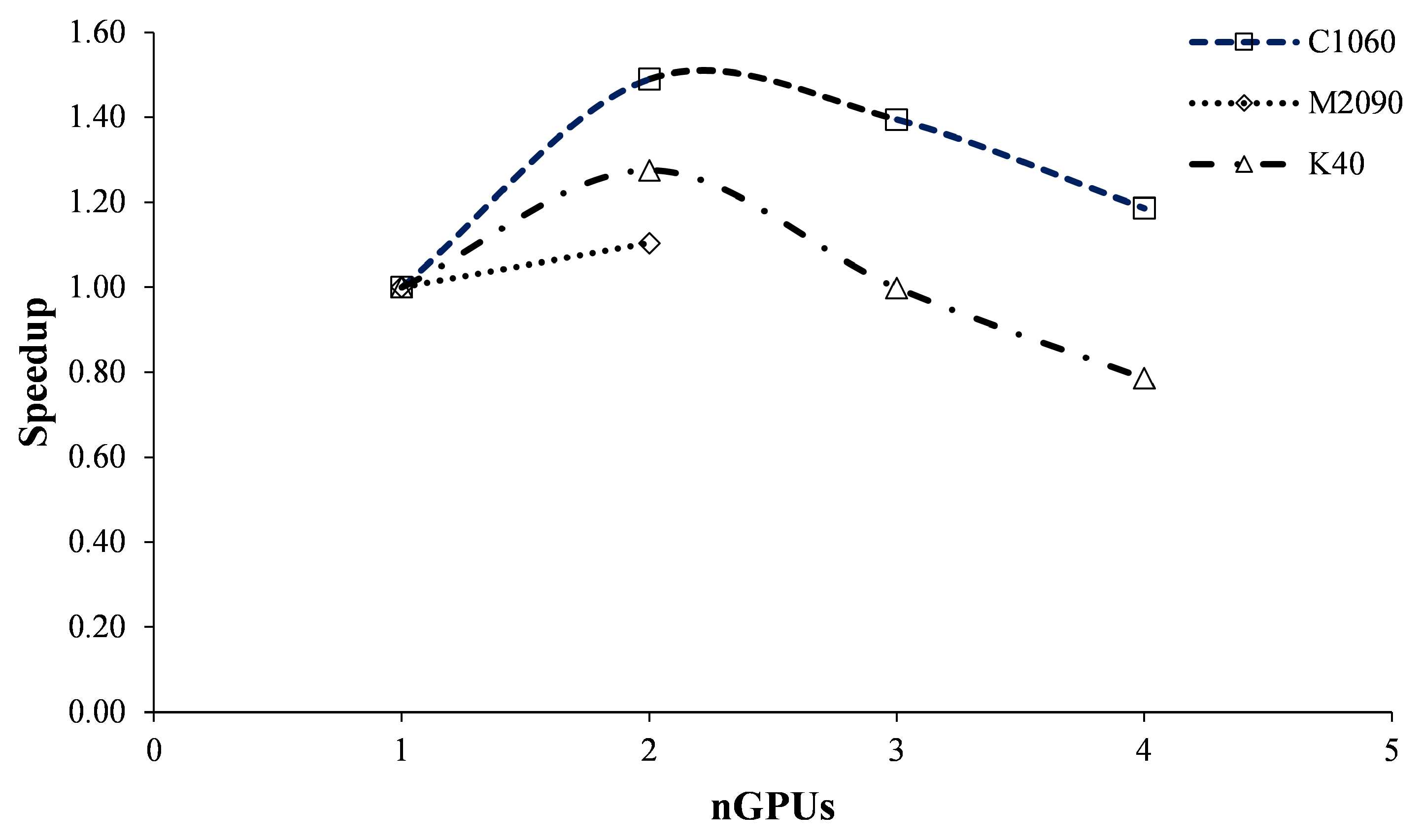
The local speedup, as calculated using Equation (
1) and based on wall clock times derived from CFD simulations across the three architectures, is depicted in
Figure 2. The experimental setup for this section was restricted to a PCG/PBiCG solver with a diagonal preconditioner and a tolerance value of
. A grid size of 981,424 cells was employed for the simulations, see
Table 2 for more details.
In all three heterogeneous architectures, speedup suddenly declines when a second GPU is used. Interestingly, the NVIDIA Tesla C1060 GPUs (in WSPAC) achieve the highest speedup despite this trend. These results suggest that further domain decomposition beyond two GPUs leads to diminishing speedup, at least for this fixed-size problem. It seems that porting too much of the computational domain to multiple GPUs leads to significant computational slowdown. This indicates that the GPU, despite being a massively parallel device, requires a substantial number of threads and a large set of elements to achieve efficient program execution.
An additional factor that must be considered, which could potentially reduce speedup, is the method of parallel computing employed by OpenFOAM. It is based on domain decomposition, whereby the geometry and associated fields are partitioned into subdomains and distributed among separate processors for solution. Parallel computing is then facilitated by the standard Message Passing Interface (MPI) [
48]. In fact, RapidCFD also leverages an MPI to manage parallel computing within the heterogeneous CPU+GPU architecture. This domain decomposition approach leads to a significant exchange of cell data between processors, as well as increased memory consumption. These aspects will be further analyzed in subsequent sections. Additionally, it has been observed that efforts to achieve strong scalability within homogeneous, single-node (CPU-only) environments can place increasing pressure on the memory subsystem as the number of MPI processes grows. This, in turn, ultimately restricts scalability [
48].
However, if base speedup is calculated, i.e., a larger wall clock time in serial is placed in the numerator of Equation (
1) for all calculations, a higher speedup is obtained by the NVIDIA Tesla K40 GPUs in WSMOL. This is because they are faster due to their greater computing power per unit, as can be observed in
Figure 3.
This last result demonstrates how speedup could lead to misleading conclusions when comparing different architectures under unequal conditions or unclear scenarios.
3.2. Performance of Linear Solvers on the Arquitectures
As a more comprehensive GPU-accelerated library, RapidCFD goes beyond being a plugin for solving sparse matrices in the OpenFOAM environment. Both linear solvers, PCG/PBiCG and GAMG, were ported to CUDA alongside discretization schemes and solution algorithms for various phenomena, e.g., compressible and incompressible fluid flows and heat transfer, to accelerate computations using GPUs. The performance of the linear solvers was analyzed by solving the same grid detailed in
Table 2 using one, two, three, and four GPUs across three distinct heterogeneous architectures.
3.2.1. GPUs and Wall Clock Time
At first glance,
Figure 4,
Figure 5 and
Figure 6 might suggest that gradient solvers are the fastest option for CFD calculations due to their superior performance. However, it would be premature to assume this advantage remains constant across different parameter configurations, as will be demonstrated later.
The data presented were obtained from CFD calculations where a tolerance value of was used for the momentum, pressure, and turbulence scalar equations at each time step. This can be considered a tight tolerance setting. The solver tolerance represents the point at which the residual becomes sufficiently small for the solution to be deemed accurate.
Upon result comparison, the computation time required to solve the same-sized problem using the GAMG linear solver was found to be nearly identical for both the Gauss–Seidel and Jacobi smoothers. Additionally, it was observed that for K40 GPUs in WSMOL and M2090 GPUs in WSGAL, the computation time increased alongside the number of GPUs and parallel domains. Conversely, the C1060 GPUs in WSPAC exhibited an inverse trend, with the computation time decreasing up to the use of four GPUs.
When employing the PCG/PBiCG linear solver with diagonal and AINV preconditioners, it was found that AINV offers the fastest performance. Interestingly, while using two GPUs reduces computation time, increasing the GPU count beyond that actually slows down the process.
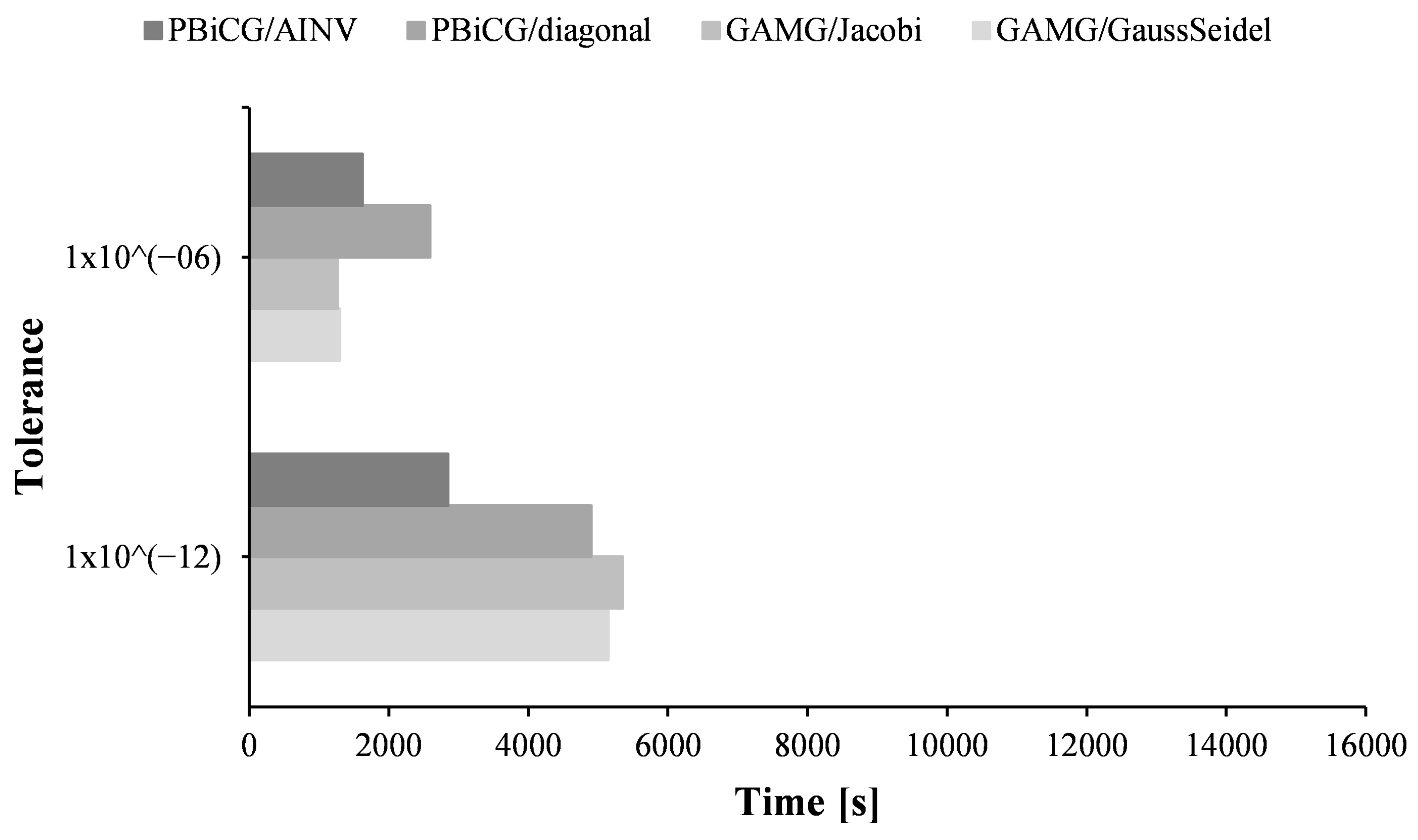
3.2.2. Tolerance Value and Wall Clock Time
When the hardware–software combination was tested with a relaxed tolerance of
, the computation time with the GAMG solver exhibited similar behavior: Gauss–Seidel and Jacobi smoothers showed negligible differences. Importantly, however, the multigrid solver outperformed the gradient solver across all architectures, refer to
Figure 7,
Figure 8 and
Figure 9.
An analysis of the plotted data reveals a clear speed advantage for multigrid linear solvers over gradient solvers when a relaxed global tolerance of approximately is used within the iterative process for each time step. However, this preference reverses when the global tolerance is tightened to smaller values, such as , as gradient solvers then regain their speed advantage.
It is crucial to note that in all test cases, the convergence criteria value was consistently maintained at throughout the computational process from setup to completion. This controlled setting bolsters the conclusion that the most efficient approach to achieve optimal speedup in GPU-accelerated CFD solutions involves pairing relaxed tolerance values with multigrid linear solvers, effectively minimizing computation time.
However, hardware limitations, which will be explored in the following section, can also exert a significant influence on the optimal selection of a linear solver.
3.3. Grid Size and Random Access Memory
Having employed a fixed problem size for the initial performance evaluation, a series of tests is now presented that is designed to identify the most significant problem size, i.e., the maximum number of cells, suitable for achieving both effective flow resolution and affordability in CFD simulations.
Table 3 summarizes all the grids used in the evaluation. Although larger grids theoretically lead to more accurate CFD solutions, as demonstrated by the convergence analysis, determining the maximum solvable problem size for GPU-accelerated CFD with limited resources remains an open question.
As HPC involves utilizing all available processing power, RapidCFD was used to measure the RAM requirements for solving CFD problems across different computer domains. These measurements were taken in both serial and parallel settings. In serial mode, each domain was solved using only one CPU core/thread and one GPU. In parallel mode, two, three, or four CPU cores/threads were used alongside an equal number of GPUs in WSPAC and WSMOL architectures. WSGAL employed a slightly different configuration with only two CPU cores and two GPUs. For each domain, both PCG/PBiCG with an AINV preconditioner and GAMG with a GaussSeidel smoother were utilized, with a tolerance value of , as this combination has been shown to be the fastest.
Building upon the previously mentioned domain decomposition approach favored by OpenFOAM, the unstructured Scotch decomposition algorithm was employed. As documented by [
49], Scotch decomposition prioritizes minimizing the size of interprocessor boundaries. However, it is prone to generating entirely new domains during redistribution, leading to a significant amount of cell data exchange between processors and, consequently, an increased memory consumption. Interestingly, inter-processor communication is integrated as a boundary condition, ensuring each cell resides solely on a unique processor via a zero-halo-layer approach, which eliminates the need for duplicated cell data near processor boundaries. It is important to note that the impact of this method transcends memory consumption and influences both computation time and speedup.
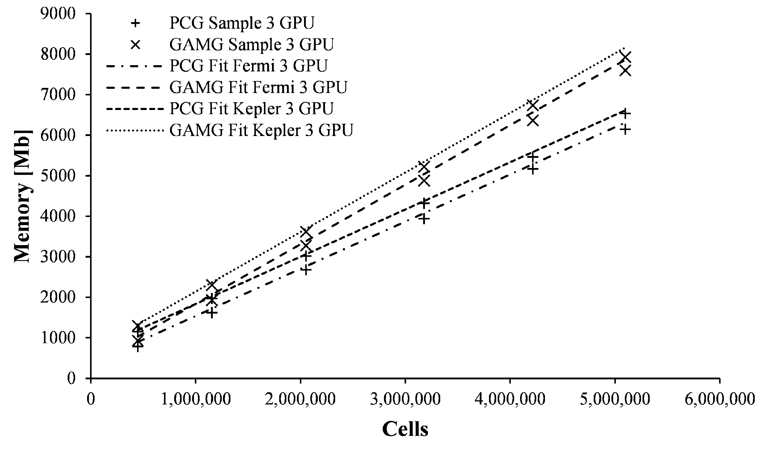
Figure 10,
Figure 11,
Figure 12 and
Figure 13 reveal a consistent pattern: regardless of grid size or whether computations are performed in serial or parallel using either PCG/PBiCG or GAMG linear solvers, the RAM requirements exhibit a straight linear behavior. This trend demonstrates that parallelizing a computational domain necessitates more RAM compared to solving it serially.
A linear regression analysis of the obtained data reveals that the memory requirements for solving problems using either PCG/PBiCG or GAMG linear solvers can be fitted and extrapolated based on hardware availability, the problem size, or alignment with convergence analysis results. Notably, for each grid size, parallelizing the computational domain consistently increases the intercept of the linear relationship while the slope remains remarkably stable. This observation has led to the proposal of four predictive equations for forecasting GPU memory requirements as a function of grid size and linear solver choice (two equations for PCG/PBiCG and two for GAMG). Notably, these equations are architecture-specific, as the results have shown a distinct influence of GPU architecture (Fermi: C1060 and M2090; Kepler: K40).
For the PCG/PBiCG gradient linear solver in a Fermi architecture:
For the PCG/PBiCG gradient linear solver in a Kepler architecture:
For the GAMG multigrid linear solver in a Fermi architecture:
Finally, for the GAMG multigrid linear solver in a Kepler architecture:
where
M is the memory requirement in Mb,
n is the number of GPUs used in the calculation and
s is the grid size (total number of cells).
As expected, memory requirements are found to vary with the linear solver chosen for each grid size. More RAM is demonstrably required by the GAMG solver compared to the PCG/PBiCG solver; however, as noted in the previous section, faster speeds are also offered by the GAMG solver when tolerance values are relaxed. Additionally, a slight increase in memory requirement has been observed when problem decomposition is parallelized when compared to serial runs, which is independent of the grid size or linear solver type. On average, 22% more RAM is required by the GAMG solver compared to the PCG/PBiCG solver. Therefore, it is concluded that the trade-off for the reduced calculation time achieved using the GAMG solver is a higher RAM usage penalty.
3.4. Open-Source GPU-Accelerated Codes: RapidCFD vs. Cufflink
The results from CFD simulations of the T-99 workbench test case, as described in previous sections, have demonstrated the advantages of employing RapidCFD and GPUs for solving CFD problems. The most significant findings pertain to memory usage and wall clock time for each CUDA-accelerated linear solver deployed within the calculation process. While only RapidCFD has been tested in multiple scenarios thus far, two reliable alternatives exist for utilizing GPUs in general-purpose CFD codes. This section will examine the cufflink plug-in for foam-extend, comparing its performance with results obtained from RapidCFD.
Before delving into the results and code comparison, several clarifications are essential:
- (i)
cufflink is a plug-in for foam-extend, meaning only its linear solvers are coded in CUDA, leaving the rest of the main code unmodified. In contrast, RapidCFD has ported numerous other parts to CUDA.
- (ii)
RapidCFD offers PCG/PBiCG and GAMG solvers, whereas cufflink’s CUDA acceleration is limited to gradient cudaCG and cudaPBiCGStab solvers.
- (iii)
The latest cufflink version for foam-extend lacks multi-GPU parallel execution capabilities, unlike RapidCFD. Consequently, comparisons of wall clock time and memory requirements were conducted by solving all cases on a single GPU of each previously used architecture.
- (iv)
To ensure consistency, a diagonal preconditioner and a tolerance value of were uniformly applied to all simulations, both in RapidCFD and cufflink. The residual target value was also held constant at .
The results, as visualized in
Figure 14, reveal that RapidCFD consistently achieves faster execution times compared to cufflink when solving problems of identical size. Conversely,
Figure 15 demonstrates cufflink’s significantly lower memory consumption for solving linear equation systems. Notably, this trade-off between solution time and memory requirements persists even when problem sizes are scaled up.
The faster execution time observed in RapidCFD compared to cufflink can be attributed to their distinct implementation approaches. cufflink operates as a plug-in for foam-extend, with only its linear solvers coded in CUDA. This means that only the linear equation system matrices are transferred through the PCI Express port and allocated to the GPUs for solving, after which the results are sent back to the CPU. This process iterates until the convergence criteria are met. Although the information package might be relatively small compared to the overall problem size (mesh information is not transferred), the transfer bus and memory allocation speed within each time step act as bottlenecks, introducing delays.
RapidCFD offers an alternative approach to circumvent the bus speed bottleneck by not only coding linear solvers in CUDA but also allocating a copy of the mesh data to the GPUs’ memory at the outset of the computation process. This strategy minimizes the amount of data transferred during each iteration, leading to a global reduction in latency, albeit at the expense of increased memory requirements.
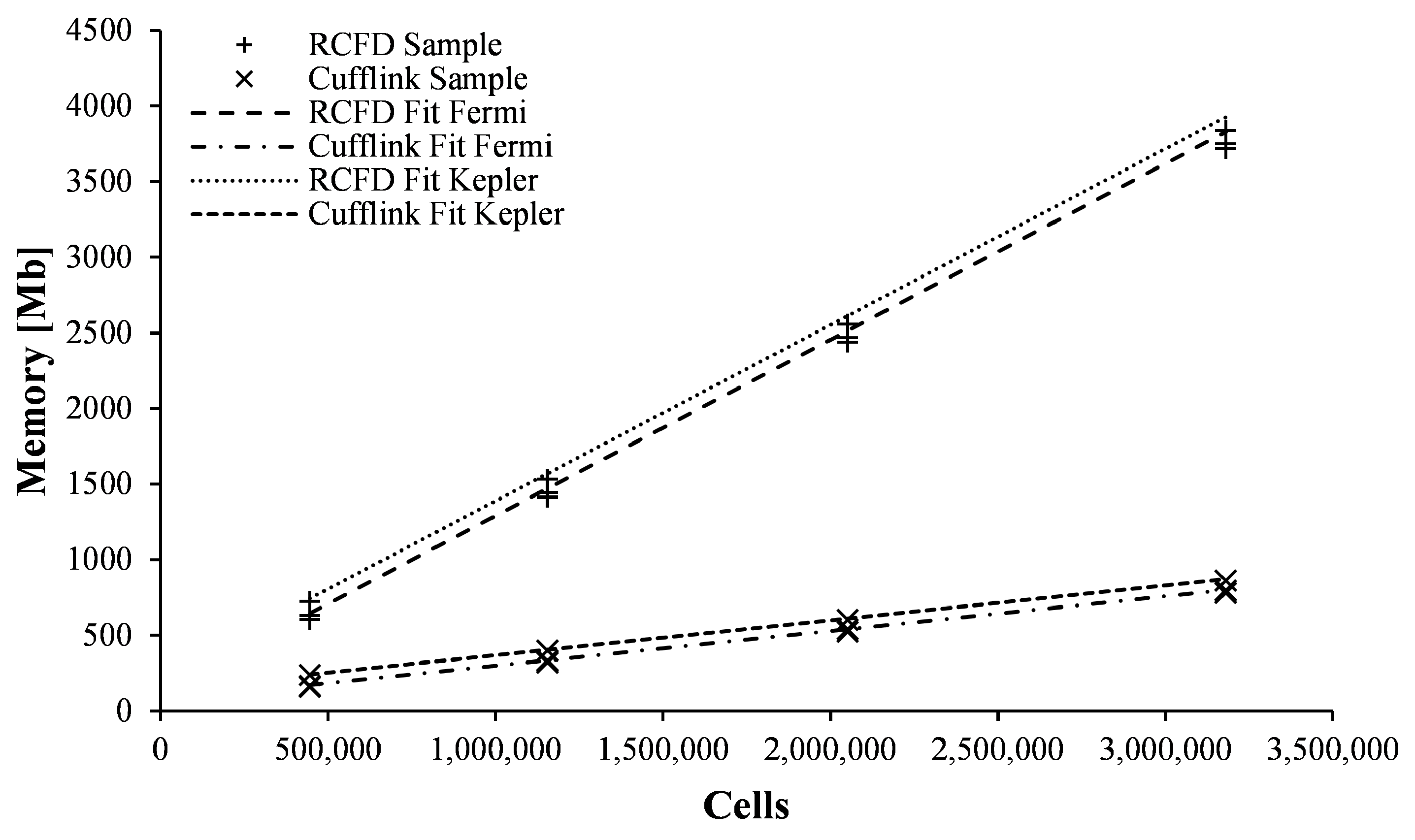
Concerning the memory requirements of cufflink on scaled problems,
Figure 16 presents the data measured from CFD computations using different grid sizes for both RapidCFD and cufflink, along with the linear regressions that fit the data.
Two equations are proposed to forecast the memory required by GPUs based on the grid size and GPU architecture.
For the Fermi architecture, the following equation can be used:
And for the Kepler architecture:
A linear behavior of memory requirements is also observed for cufflink, suggesting its potential to solve larger grid size problems compared to RapidCFD, albeit with a trade-off of longer computation times.
4. Discussion
Figure 4,
Figure 5,
Figure 6,
Figure 7,
Figure 8 and
Figure 9 show that the AINV preconditioner exhibits faster convergence compared to the diagonal preconditioner for the PCG/PBiCG linear solvers. This difference can be attributed to the underlying formulation of the preconditioning techniques. As noted by van der Vorst [
50], CG methods project the original problem onto a smaller Krylov subspace for solution approximation. Preconditioning plays a key role in improving the convergence rate of these methods by transforming the system into one with better spectral properties. This transformation allows for the achievement of an accurate solution with fewer iterations, reducing the overall computational time. Consequently, the number of iterations needed for convergence becomes the primary factor determining the computational cost. The diagonal preconditioner, as described by Saad [
46], utilizes the diagonal entries of the original matrix. While its implementation is straightforward, it may not be effective for systems lacking strong diagonal dominance. In contrast, the AINV preconditioner directly approximates the matrix’s inverse, leading to excellent convergence properties for specific problems.
Multigrid methods employ a hierarchy of grids with varying levels of coarseness, as explained by Wesseling [
51]. Coarser grids address low-frequency errors, while finer grids handle high-frequency errors, enabling efficient error reduction across different scales. Within each multigrid cycle, smoothers are applied on the finer grids to reduce high-frequency errors. The Jacobi smoother updates each solution point based on the values of its immediate neighbors, while the Gauss–Seidel smoother iteratively updates solution points using the most recently updated values of neighboring points during the current iteration, potentially leading to faster convergence compared to Jacobi [
52].
Figure 4,
Figure 5,
Figure 6,
Figure 7,
Figure 8 and
Figure 9 illustrate that both smoothers exhibit similar performance in terms of solution time for the same problem.
Multigrid methods generally exhibit optimal convergence rates, meaning the error is reduced by a constant factor with each iteration. This characteristic can lead to fewer iterations compared to CG methods, especially for well-structured problems [
51]. However, the overhead associated with grid transfers and hierarchy setup can contribute to a higher cost per iteration.
Figure 4,
Figure 5 and
Figure 6 showcase this phenomenon, where using a tolerance of
results in a longer computation time for the GAMG linear solver compared to PCG/PBiCG. Nonetheless, when a looser tolerance of
was used, as shown in
Figure 7,
Figure 8 and
Figure 9, the GAMG linear solver became faster than PCG/PBiCG.
As expected due to the nature of CG and multigrid methods,
Figure 10,
Figure 11,
Figure 12 and
Figure 13 demonstrate that the memory requirement scales linearly with the problem size. Additionally, multigrid methods require storing the solution on multiple grids and storing the data structures for the grid hierarchy, resulting in higher memory requirements compared to CG methods [
51]. This observation is further supported by
Figure 10,
Figure 11,
Figure 12 and
Figure 13, where PCG/PBiCG exhibits lower memory requirements compared to GAMG linear solvers.
5. Implications
Segregated solvers encounter increased challenges when addressing transient problems, which require time-stepping and introduce additional iterations that can hinder convergence. Furthermore, rapid changes in flow parameters over time can strengthen the coupling between variables, potentially further slowing convergence. Compressible flows necessitate the solution of additional equations, including those governing thermal energy conservation and the relationship between density, temperature, and pressure. While these algorithms can be adapted for heat transfer problems by solving the energy equation alongside momentum and pressure correction, they are not inherently designed to directly model buoyancy phenomena. Simulating multiphase flows (e.g., liquid–gas, solid–liquid) introduces further complexity, requiring transport equations for phase fractions and models for interfacial interactions. Additionally, cavitation, characterized by rapid pressure changes and vapor bubble formation and collapse, presents even more equations and numerical challenges. Both cavitation and multiphase flows necessitate the use of specialized models, such as volume-of-fluid and level-set methods, which extend beyond the capabilities of basic segregated solvers. Further details can be found in [
44,
52].
As mentioned earlier, the SIMPLE algorithm is a general numerical procedure for calculating heat, mass, and momentum transfer in the steady state. The Pressure-Implicit Splitting Operator (PISO) algorithm is used for transient problems and handles the pressure–velocity coupling of implicitly discretized, time-dependent fluid flow equations. It utilizes the splitting of operations in the solution process to achieve solutions close to the exact difference equations [
53,
54]. The main differences between SIMPLE and PISO lie in the included time derivation terms and the consistency of the pressure–velocity coupling equation. Most of OpenFOAM’s fluid solver modules use SIMPLE. PIMPLE, a combination of PISO and SIMPLE algorithms, couples mass and momentum conservation equations, enabling larger time steps and higher Courant numbers [
55]. Both PISO and PIMPLE are suitable for transient problems, while SIMPLE is used for steady-state problems. Although all three algorithms solve the same governing equations (continuity, momentum, and energy), their key difference lies in how they iterate through equations [
38,
56].
Despite their differences in handling specific phenomena, SIMPLE, PISO, and PIMPLE share the core principles of the segregated approach, potentially exhibiting similar performance and computational costs. Factors like preconditioning, multigrid methods, and solver selection all influence the computational cost. Therefore, results related to memory bandwidth might be similar when using pressure-based solution algorithms like these. However, the computation time would be the most affected, especially when simulating complex phenomena like multiphase and cavitation flows due to the transient treatment and additional equations required in the solution. Nevertheless, findings from this work can still be applied to similar problems in the turbomachinery field.
6. Limitations
Official OpenFOAM versions undergo constant development and maintenance by Technical Committees and the OpenFOAM community, with new updates released twice a year. RapidCFD, although derived from OpenFOAM 2.3.1, has remained largely unchanged since its release. This means that new developments related to algorithms, linear solvers, boundary conditions, and turbulence models, among others, are not ported from newer OpenFOAM versions to RapidCFD. Currently, RapidCFD functions as a standalone solver, requiring pre-processing and post-processing to be performed in OpenFOAM (official or community versions) and ParaView, respectively. This can potentially create difficulties if users wish to directly utilize new tools (boundary conditions, turbulence models, etc.). In such cases, extra effort would be needed to port these features to RapidCFD. On the other hand, foam-extend offers extensions and additional features. These features include dynamic mesh and topological change support, turbomachinery extensions, implicitly coupled conjugate heat transfer, and other physics coupling capabilities. However, its GPU-accelerated library has been shown to be slower than the RapidCFD fork.
All available options remain open source and are supported by community developments, with some communities being larger than others. Therefore, modifications can be made to better suit the problem under analysis. Ultimately, the decision of which code to use depends on the problem’s complexity and, as it has been shown, available hardware resources.
7. Conclusions
This study has investigated the acceleration of a turbomachinery numerical model using GPU-accelerated libraries for the OpenFOAM environment. Regarding the performance of software/hardware combinations, it was shown that the optimal strategy employs the GAMG solver with relaxed tolerance values. This configuration achieves reduced calculation times without compromising results compared to PCG/PBiCG. However, it was also observed that the GAMG linear solver requires approximately 22% more RAM on the GPUs compared to PCG/PBiCG. This increased memory demand can be considered as a trade-off for the improved solution speed, as the GAMG solver is up to 70% faster than PCG/PBiCG. Finally, it was observed that parallelizing a computational domain incurs a memory cost in exchange for a reduced calculation time. To address this trade-off, a set of equations was proposed to estimate the required RAM for each linear solver configuration.
The obtained results are highly promising. They suggest that porting larger portions of CFD simulations to GPUs could lead to significant computation accelerations, particularly for complex industrial flows like those encountered in a turbine testing laboratory.
Author Contributions
Conceptualization, D.M.-H. and S.R.G.-G.; Methodology, D.M.-H., S.R.G.-G., N.D.H.-S. and P.G.-A.; Software, D.M.-H.; Validation, D.M.-H. and S.R.G.-G.; Formal Analysis, D.M.-H. and S.R.G.-G.; Investigation, D.M.-H. and S.R.G.-G.; Resources, S.R.G.-G. and J.J.P.-I.; Data Curation, D.M.-H.; Writing—Original Draft Preparation, D.M.-H., S.R.G.-G. and P.G.-A.; Writing—Review and Editing, D.M.-H., S.R.G.-G., N.D.H.-S., P.G.-A., J.J.P.-I. and F.J.D.-M.; Visualization, D.M.-H. and S.R.G.-G.; Supervision, S.R.G.-G., N.D.H.-S., J.J.P.-I. and F.J.D.-M.; Project Administration, S.R.G.-G.; Funding Acquisition, S.R.G.-G., J.J.P.-I. and F.J.D.-M. All authors have read and agreed to the published version of the manuscript.
Funding
The author(s) disclosed receipt of the following financial support for the research of this article: this work was supported by scholarship (298290) from the Consejo Nacional de Humanidades, Ciencias y Tecnologías (CONAHCYT).
Data Availability Statement
The data used and presented in this research could be made available on request.
Acknowledgments
The authors express their gratitude to the Universidad Michoacana de San Nicolás de Hidalgo (UMSNH) and its Faculty of Mechanical Engineering for providing access to their facilities, laboratories, materials, and digital resources, particularly during the challenging times of the COVID-19 pandemic. We would also like to thank Aula CIMNE Morelia for their technical support.
Conflicts of Interest
The authors declare no conflicts of interest.
Abbreviations
The following abbreviations are used in this manuscript:
| GPU | Graphic Processor Unit |
| CFD | Computational Fluids Dynamics |
| CUDA | Compute Unified Device Architecture |
| OpenFOAM | Open Field Operation and Manipulation |
| HPC | High-Performance Computing |
| CPU | Central Processing Unit |
| RAM | Random Access Memory |
| cufflink | Cuda For FOAM Link |
| ERCOFTAC | European Research Community on Flow Turbulence and Combustion |
| SIMPLE | Semi Implicit Method for Pressure-Linked Equations |
| FVM | Finite Volume Method |
| PCG | Preconditioned Conjugate Gradient |
| PBiCG | Preconditioned Bi-Conjugate Gradient |
| GAMG | Generalized Geometric Algebraic Multi-Grid |
| AINV | Approximate Inverse |
| CG | Conjugated Gradient |
| BiCG | Bi-Conjugate Gradient |
| GMG | Geometric Multi-Grid |
| AMG | Algebraic Multi-Grid |
| MPI | Message Passing Interface |
| PISO | Pressure-Implicit Splitting Operator |
References
- Malecha, Z.; Mirosław, Ł.; Tomczak, T.; Koza, Z.; Matyka, M.; Tarnawski, W.; Szczerba, D. GPU-based simulation of 3D blood flow in abdominal aorta using OpenFOAM. Arch. Mech. 2011, 63, 137–161. [Google Scholar]
- He, Q.; Chen, H.; Feng, J. Acceleration of the OpenFOAM-based MHD solver using graphics processing units. Fusion Eng. Des. 2015, 101, 88–93. [Google Scholar] [CrossRef]
- Horváth, Z.; Perdigão, R.A.; Waser, J.; Cornel, D.; Konev, A.; Blöschl, G. Kepler shuffle for real-world flood simulations on GPUs. Int. J. High Perform. Comput. Appl. 2016, 30, 379–395. [Google Scholar] [CrossRef]
- AbdelMigid, T.A.; Saqr, K.M.; Kotb, M.A.; Aboelfarag, A.A. Revisiting the lid-driven cavity flow problem: Review and new steady state benchmarking results using GPU accelerated code. Alex. Eng. J. 2017, 56, 123–135. [Google Scholar] [CrossRef]
- Glimberg, S.L.; Engsig-Karup, A.P.; Olson, L.N. A massively scalable distributed multigrid framework for nonlinear marine hydrodynamics. Int. J. High Perform. Comput. Appl. 2019, 33, 855–868. [Google Scholar] [CrossRef]
- Fernandez, G.; Mendina, M.; Usera, G. Heterogeneous Computing (CPU–GPU) for Pollution Dispersion in an Urban Environment. Computation 2020, 8, 3. [Google Scholar] [CrossRef]
- Piscaglia, F.; Ghioldi, F. GPU Acceleration of CFD Simulations in OpenFOAM. Aerospace 2023, 10, 792. [Google Scholar] [CrossRef]
- Liu, X.; Zhong, Z.; Xu, K. A Hybrid Solution Method for CFD Applications on GPU-Accelerated Hybrid HPC Platforms. Future Gener. Comput. Syst. 2016, 56, 759–765. [Google Scholar] [CrossRef]
- Nocente, A.; Arslan, T.; Jasiński, D.; Nielsen, T. A Study of Flow inside a Centrifugal Pump: High Performance Numerical Simulations Using GPU cards. In Proceedings of the 16th International Symposium on Transport Phenomena and Dynamics of Rotating Machinery 2016, Honolulu, HI, USA, 10–15 April 2016. [Google Scholar]
- Molinero, D.; Galván, S.; Pacheco, J.; Herrera, N. Multi GPU Implementation to Accelerate the CFD Simulation of a 3D Turbo–Machinery Benchmark Using the RapidCFD Library. In Proceedings of the Supercomputing; Torres, M., Klapp, J., Eds.; Springer International Publishing: Berlin/Heidelberg, Germany, 2019; pp. 173–187. [Google Scholar] [CrossRef]
- Molinero, D.; Galván, S.; Domínguez, F.; Ibarra, L.; Solorio, G. Francis 99 CFD through RapidCFD accelerated GPU code. IOP Conf. Ser. Earth Environ. Sci. 2021, 774, 012016. [Google Scholar] [CrossRef]
- Poli, F.; Marconcini, M.; Pacciani, R.; Magarielli, D.; Spano, E.; Arnone, A. Exploiting GPU-Based HPC Architectures to Accelerate an Unsteady CFD Solver for Turbomachinery Applications. In Turbo Expo: Power for Land, Sea, and Air; ASME: New York, NY, USA, 2022; p. V10CT32A035. [Google Scholar] [CrossRef]
- Culpo, M. Current Bottlenecks in the Scalability of OpenFOAM on Massively Parallel Clusters; Technical Report; Partnership for Advanced Computing in Europe, Zenodo: Geneve, Switzerland, 2012. [Google Scholar] [CrossRef]
- Jasak, H. OpenFOAM: Open source CFD in research and industry. Int. J. Nav. Archit. Ocean. Eng. 2009, 1, 89–94. [Google Scholar] [CrossRef]
- AlOnazi, A. Design and Optimization of OpenFOAM-Based CFD Applications for Modern Hybrid and Heterogeneous HPC Platforms. Ph.D. Thesis, King Abdullah University of Science and Technology, Thuwal, Saudi Arabia, 2014. [Google Scholar] [CrossRef]
- Che, S.; Skadron, K. BenchFriend: Correlating the performance of GPU benchmarks. Int. J. High Perform. Comput. Appl. 2014, 28, 238–250. [Google Scholar] [CrossRef]
- Bna, S.; Spisso, I.; Olesen, M.; Rossi, G. PETSc4FOAM: A Library to Plug-in PETSc into the OpenFOAM Framework; Technical Report; Partnership for Advanced Computing in Europe, Zenodo: Geneve, Switzerland, 2020. [Google Scholar] [CrossRef]
- Aissa, M.H. GPU-Accelerated CFD Simulations for Turbomachinery Design Optimization. Ph.D. Thesis, Delft University of Technology, Delft, The Netherlands, 2017. [Google Scholar] [CrossRef]
- Simflow, T. RapidCFD. OpenFOAM Running on GPU. 2021. Available online: https://sim-flow.com/rapid-cfd-gpu/ (accessed on 28 October 2021).
- Jasiński, D. Adapting OpenFOAM for massively parallel GPU architecture. In Proceedings of the 3rd OpenFOAM User Conference 2015, Stuttgart, Germany, 19–21 October 2015. [Google Scholar]
- Singh, S.N.; Seshadri, V.; Chandel, S.; Gaikwad, M. Analysis of the Improvement in Performance Characteristics of S-Shaped Rectangular Diffuser by Momentum Injection Using Computational Fluid Dynamics. Eng. Appl. Comput. Fluid Mech. 2009, 3, 109–122. [Google Scholar] [CrossRef]
- Drainy, Y.A.E.; Saqr, K.M.; Aly, H.S.; Jaafar, M.N.M. CFD Analysis of Incompressible Turbulent Swirling Flow through Zanker Plate. Eng. Appl. Comput. Fluid Mech. 2009, 3, 562–572. [Google Scholar] [CrossRef]
- Andersson, U. Turbine-99 - Experiments on Draft Tube Flow (Test Case T). In Proceedings of the Turbine-99: Workshop on Draft Tube Flow, Porjus, Sweden, 20–23 June 1999. Number 2000:11 in Teknisk Rapport/Luleå Tekniska Universitet, 2000. [Google Scholar]
- Andersson, U.; Karlsson, R. Quality aspects of the Turbine 99 draft tube experiment. In Proceedings of the Turbine-99: Workshop on Draft Tube Flow, Porjus, Sweden, 20–23 June 1999. Number 2000:11 in Teknisk Rapport/Luleå Tekniska Universitet, 2000. [Google Scholar]
- Fortin, M.; Nennemann, B.; Houde, S.; Deschenes, C. Numerical study of the flow dynamics at no-load operation for a high head Francis turbine at model scale. IOP Conf. Ser. Earth Environ. Sci. 2019, 240, 022023. [Google Scholar] [CrossRef]
- Fortin, M.; Nennemann, B.; Houde, S. Characterization of no-load conditions for a high head Francis turbine based on the swirl level. IOP Conf. Ser. Earth Environ. Sci. 2022, 1079, 012010. [Google Scholar] [CrossRef]
- Gilis, A.; Coulaud, M.; Munoz, A.; Maciel, Y.; Houde, S. Experimental study of the flow of the Tr-Francis turbine along the no-load curve. IOP Conf. Ser. Earth Environ. Sci. 2022, 1079, 012019. [Google Scholar] [CrossRef]
- Wack, J.; Grübel, M.; Conrad, P.; Locquenghien, F.V.; Jester-Zürker, R.; Riedelbauch, S. Numerical investigation of the impact of cavitation on the pressure fluctuations in a Francis turbine at deep part load conditions. IOP Conf. Ser. Earth Environ. Sci. 2022, 1079, 012044. [Google Scholar] [CrossRef]
- Junginger, B.; Riedelbauch, S. Analysis of a propeller turbine operated in a full load operating point. IOP Conf. Ser. Earth Environ. Sci. 2019, 405, 012028. [Google Scholar] [CrossRef]
- Joßberger, S.; Riedelbauch, S. Scale-Resolving Hybrid RANS-LES Simulation of a Model Kaplan Turbine on a 400-Million-Element Mesh. Int. J. Turbomach. Propuls. Power 2023, 8, 26. [Google Scholar] [CrossRef]
- Drepper, U. What every programmer should know about memory. Red Hat Inc. 2007, 11, 2007. [Google Scholar]
- CUDA C++ Programming Guide. Release 12.3; NVIDIA Corporation: Santa Clara, CA, USA, 2024.
- Gebart, R.; Gustavsson, H.; Karlsson, R. (Eds.) Proceedings of Turbine-99: Workshop on Draft Tube Flow, Porjus, Sweden, 20–23 June 1999; Number 2000:11 in Teknisk Rapport; Luleå Tekniska Universitet: Luleå, Sweden, 2000. [Google Scholar]
- Engström, T.F.; Gustavsson, H.; Karlsson, R. (Eds.) Proceedings of Turbine-99-Workshop 2: The Second ERCOFTAC Workshop on Draft Tube Flow, Älvkarleby, Sweden, 18–20 June 2001; Luleå University of Technology: Luleå, Sweden, 2002. [Google Scholar]
- Cervantes, M.; Engström, F.; Gustavsson, H. (Eds.) Turbine-99 III: Proceedings of the Third on Draft Tube Flow, Porjus, Sweden, 8–9 December 2005; Number 2005:20 in Forskningsrapport; Luleå Tekniska Universitet: Luleå, Sweden, 2005. [Google Scholar]
- Cervantes, M. Turbine-99 III, 3rd IAHR workshop on draft tube flow. ERCOFTAC Bull. 2006, 69, 9–19. [Google Scholar]
- Patankar, S.; Spalding, D. A calculation procedure for heat, mass and momentum transfer in three-dimensional parabolic flows. Int. J. Heat Mass Transf. 1972, 15, 1787–1806. [Google Scholar] [CrossRef]
- OpenFOAM. The Open Source CFD Toolbox. User Guide; OpenCFD Limited: Bracknell, UK, 2017. [Google Scholar]
- Khajeh-Saeed, A.; Perot, J.B. Computational Fluid Dynamics Simulations Using Many Graphics Processors. Comput. Sci. Eng. 2012, 14, 10–19. [Google Scholar] [CrossRef]
- Launder, B.; Spalding, D. The numerical computation of turbulent flows. Comput. Methods Appl. Mech. Eng. 1974, 3, 269–289. [Google Scholar] [CrossRef]
- Cervantes, M.; Engström, T.F. Influence of boundary conditions using factorial design. In Proceedings of the Turbine-99 II: Workshop on Draft Tube Flow, Älvkarleby, Sweden, 18–20 June 2001. [Google Scholar]
- Andersson, U. Test case T-some news results and updates since workshop 1. In Proceedings of the Turbine-99-Workshop 2: The Second ERCOFTAC Workshop on Draft Tube Flow, Älvkarleby, Sweden, 18–20 June 2001; pp. 1–11. [Google Scholar]
- Versteeg, H.K.; Malalasekera, W. An Introduction to Computational Fluid Dynamics: The Finite Volume Method; Pearson Education: Harlow, UK, 2007. [Google Scholar]
- Moukalled, F.; Mangani, L.; Darwish, M. The Finite Volume Method in Computational Fluid Dynamics; Springer International Publishing: Cham, Switzerland, 2016; p. 791. [Google Scholar] [CrossRef]
- Lu, C.; Jiao, X.; Missirlis, N. A hybrid geometric algebraic multigrid method with semi-iterative smoothers. Numer. Linear Algebra Appl. 2014, 21, 221–238. [Google Scholar] [CrossRef]
- Saad, Y. Iterative Methods for Sparse Linear Systems, 2nd ed.; Society for Industrial and Applied Mathematics: Philadelphia, PA, USA, 2003. [Google Scholar] [CrossRef]
- Navarro, C.A.; Hitschfeld-Kahler, N.; Mateu, L. A Survey on Parallel Computing and its Applications in Data-Parallel Problems Using GPU Architectures. Commun. Comput. Phys. 2014, 15, 285–329. [Google Scholar] [CrossRef]
- Garcia-Gasulla, M.; Banchelli, F.; Peiro, K.; Ramirez-Gargallo, G.; Houzeaux, G.; Ben Hassan Saïdi, I.; Tenaud, C.; Spisso, I.; Mantovani, F. A Generic Performance Analysis Technique Applied to Different CFD Methods for HPC. Int. J. Comput. Fluid Dyn. 2020, 34, 508–528. [Google Scholar] [CrossRef]
- Rettenmaier, D.; Deising, D.; Ouedraogo, Y.; Gjonaj, E.; De Gersem, H.; Bothe, D.; Tropea, C.; Marschall, H. Load balanced 2D and 3D adaptive mesh refinement in OpenFOAM. SoftwareX 2019, 10, 100317. [Google Scholar] [CrossRef]
- van der Vorst, H.A. Iterative Krylov Methods for Large Linear Systems; Cambridge Monographs on Applied and Computational Mathematics; Cambridge University Press: Cambridge, UK, 2003. [Google Scholar] [CrossRef]
- Wesseling, P. An Introduction to Multigrid Methods; John Wiley & Sons Ltd.: Chichester, UK, 1992. [Google Scholar]
- Ferziger, J.H.; Perić, M.; Street, R.L. The Finite Volume Method in Computational Fluid Dynamics; Springer: Cham, Switzerland, 2019. [Google Scholar] [CrossRef]
- Issa, R. Solution of the implicitly discretised fluid flow equations by operator-splitting. J. Comput. Phys. 1985, 62, 40–65. [Google Scholar] [CrossRef]
- Issa, R.; Gosman, A.; Watkins, A. The computation of compressible and incompressible recirculating flows by a non-iterative implicit scheme. J. Comput. Phys. 1986, 62, 66–82. [Google Scholar] [CrossRef]
- Holzmann, T. Mathematics, Numerics, Derivations and OpenFOAM; Holzmann CFD: Bad Wörishofen, Germany, 2020. [Google Scholar] [CrossRef]
- Greenshields, C. OpenFOAM v11 User Guide; The OpenFOAM Foundation: London, UK, 2023. [Google Scholar]
Figure 1.
Structured mesh geometry of the ERCOFTAC turbine T-99 draft tube for simulations.
Figure 1.
Structured mesh geometry of the ERCOFTAC turbine T-99 draft tube for simulations.
Figure 2.
Local speedup achieved with PCG/PBiCG solver across heterogeneous architectures using RapidCFD to solve the ERCOFTAC Turbine T-99 draft tube.
Figure 2.
Local speedup achieved with PCG/PBiCG solver across heterogeneous architectures using RapidCFD to solve the ERCOFTAC Turbine T-99 draft tube.
Figure 3.
Base speedup achieved with PCG/PBiCG solver across heterogeneous architectures using RapidCFD to solve the ERCOFTAC Turbine T-99 draft tube.
Figure 3.
Base speedup achieved with PCG/PBiCG solver across heterogeneous architectures using RapidCFD to solve the ERCOFTAC Turbine T-99 draft tube.
Figure 4.
Comparison of wall clock time using different linear solvers, and preconditioners/smoothers on WSMOL.
Figure 4.
Comparison of wall clock time using different linear solvers, and preconditioners/smoothers on WSMOL.
Figure 5.
Comparison of wall clock time using different linear solvers, and preconditioners/smoothers on WSGAL.
Figure 5.
Comparison of wall clock time using different linear solvers, and preconditioners/smoothers on WSGAL.
Figure 6.
Comparison of wall clock time using different linear solvers, and preconditioners/smoothers on WSPAC.
Figure 6.
Comparison of wall clock time using different linear solvers, and preconditioners/smoothers on WSPAC.
Figure 7.
Comparison of wall clock time using different tolerance values, linear solvers, and preconditioners/smoothers on WSMOL.
Figure 7.
Comparison of wall clock time using different tolerance values, linear solvers, and preconditioners/smoothers on WSMOL.
Figure 8.
Comparison of wall clock time using different tolerance values, linear solvers, and preconditioners/smoothers on WSGAL.
Figure 8.
Comparison of wall clock time using different tolerance values, linear solvers, and preconditioners/smoothers on WSGAL.
Figure 9.
Comparison of wall clock time using different tolerance values, linear solvers, and preconditioners/smoothers on WSPAC.
Figure 9.
Comparison of wall clock time using different tolerance values, linear solvers, and preconditioners/smoothers on WSPAC.
Figure 10.
Predictable memory growth: linear scaling of RAM use in GPU-accelerated CFD across grid sizes and solvers using one GPU.
Figure 10.
Predictable memory growth: linear scaling of RAM use in GPU-accelerated CFD across grid sizes and solvers using one GPU.
Figure 11.
Predictable memory growth: linear scaling of RAM use in GPU-accelerated CFD across grid sizes, solvers, and parallelization using two GPUs.
Figure 11.
Predictable memory growth: linear scaling of RAM use in GPU-accelerated CFD across grid sizes, solvers, and parallelization using two GPUs.
Figure 12.
Predictable memory growth: linear scaling of RAM use in GPU-accelerated CFD across grid sizes, solvers, and parallelization using three GPUs.
Figure 12.
Predictable memory growth: linear scaling of RAM use in GPU-accelerated CFD across grid sizes, solvers, and parallelization using three GPUs.
Figure 13.
Predictable memory growth: linear scaling of RAM use in GPU-accelerated CFD across grid sizes, solvers, and parallelization using four GPUs.
Figure 13.
Predictable memory growth: linear scaling of RAM use in GPU-accelerated CFD across grid sizes, solvers, and parallelization using four GPUs.
Figure 14.
Wall clock time for different grid sizes: RapidCFD vs. cufflink.
Figure 14.
Wall clock time for different grid sizes: RapidCFD vs. cufflink.
Figure 15.
Memory consumption for different grid sizes: RapidCFD vs. cufflink.
Figure 15.
Memory consumption for different grid sizes: RapidCFD vs. cufflink.
Figure 16.
Memory use scaling in CFD across grid sizes: RapidCFD and cufflink.
Figure 16.
Memory use scaling in CFD across grid sizes: RapidCFD and cufflink.
Table 1.
Hardware features.
Table 1.
Hardware features.
| WSPAC | WSGAL | WSMOL |
|---|
| | CPU | |
| 2 × Intel Xeon E5504, 2.0 GHz | 2 × Intel Xeon L5639, 2.13 GHz | 2 × Intel Xeon E5-2640 v2, 2.0 GHz |
| 4 cores per processor/4 threads | 6 cores per processor/12 threads | 8 cores per processor/16 threads |
| 12 GB Memory DDR3, 1060 Hz | 24 GB Memory DDR3, 1060 Hz | 64 GB Memory DDR3, 1600 Hz |
| | GPU | |
| 4 × Nvidia Tesla C1060 | 2 × Nvidia Tesla M2090 | 4 × Nvidia Tesla K40 |
| 240 CUDA cores, 1.296 GHz | 512 CUDA cores, 1.3 GHz | 2880 CUDA cores, 745 MHz |
| 4 GB Memory GDDR3, 800 MHz | 6 GB Memory GDDR5, 1.85 GHz | 12 GB Memory GDDR5, 3 GHz |
Table 2.
Main features of the mesh used for speedup analysis.
Table 2.
Main features of the mesh used for speedup analysis.
| Parameter | Value |
|---|
| Cells (s) | 981,424 |
| Cell type | hexahedra |
| Max aspect ratio | 85.2749 |
| Max non-orthogonality | 77.9564 |
| Average non-orthogonality | 19.0842 |
| Max skewness | 2.84655 |
Table 3.
Summary of CFD grids used in GPU acceleration evaluation for RAM analysis.
Table 3.
Summary of CFD grids used in GPU acceleration evaluation for RAM analysis.
| Mesh | Cells (s) | Cell Type | Max Aspect Ratio | Max Non-Orthogonality | Average Non-Orthogonality | Max Skewness |
|---|
| 1 | 446,820 | hexahedra | 130.19 | 85.9322 | 18.3519 | 1.12942 |
| 2 | 1,154,832 | hexahedra | 108.736 | 86.2163 | 17.3094 | 1.17965 |
| 3 | 2,051,712 | hexahedra | 128.456 | 86.4505 | 17.5097 | 1.41215 |
| 4 | 3,179,080 | hexahedra | 126.468 | 86.1913 | 17.0782 | 1.51821 |
| 5 | 4,215,904 | hexahedra | 128.673 | 86.2943 | 16.8987 | 1.56909 |
| 6 | 5,096,736 | hexahedra | 140.634 | 86.4107 | 16.7642 | 1.61848 |
| Disclaimer/Publisher’s Note: The statements, opinions and data contained in all publications are solely those of the individual author(s) and contributor(s) and not of MDPI and/or the editor(s). MDPI and/or the editor(s) disclaim responsibility for any injury to people or property resulting from any ideas, methods, instructions or products referred to in the content. |
© 2024 by the authors. Licensee MDPI, Basel, Switzerland. This article is an open access article distributed under the terms and conditions of the Creative Commons Attribution (CC BY) license (https://creativecommons.org/licenses/by/4.0/).


 ,
, 


