Recent Developments in Using a Modified Transfer Matrix Method for an Automotive Exhaust Muffler Design Based on Computation Fluid Dynamics in 3D

Abstract

The present work aims to investigate the newly modified transfer matrix method (MTMM) to predict an automotive exhaust muffler’s transmission loss (AEMTL). The MTMM is a mixed method between a 3D-CFD (Computation Fluid Dynamics in 3D), namely AVL FIRE^TM M Engine (process-safe 3D-CFD Simulations of Internal Combustions Engines), and the classic TMM for the exhaust muffler. For all the continuous and discontinuous sections of the exhaust muffler, the Mach number of the cross-section, the temperature, and the type of discontinuity of the exhaust gas flow were taken into consideration to evaluate the specific elements of the acoustic quadrupole that define the MTMM coupled with AVL FIRE^TM M Engine for one given muffler exhaust. Also, the perforations of intermediary ducts were considered in the new MTMM (AVL FIRE^TM M Engine linked with TMM) to predict the TL (transmission loss) of an automotive exhaust muffler with three expansion chambers. The results obtained for the TL in the frequency range 0.1-4 kHz agree with the experimental results published in the literature. The TMM was improved by adding the AVL FIRE^TM M Engine as a valuable tool in designing the automotive exhaust muffler (AEM).

1. Introduction

Mufflers are commonly used in a wide variety of applications. Industrial flow ducts and internal combustion engines frequently use silencing elements to attenuate the noise levels carried by the fluids and radiated to the outside atmosphere by the exhausts. Designing a complete muffler system is usually very complex because each element is selected considering its exceptional acoustic performance and interaction effects on the entire system’s performance. For the frequency analysis of the muffler, it is very convenient to use the transfer matrix method (TMM), as stated by the authors of [1], whose paper presents a detailed overview of the TMM’s use two decades ago so as to analyze the mufflers’ acoustics properties and the TL. Articles [2,3] shed light on the transfer function method and realistic models to predict and measure the sound propagation in ducts. Mechel presented and developed, in general, the mathematical relations for the TMM [4], while Munjal in [5] (pp. 104–152) dealt with the aeroacoustics of exhaust mufflers designed for internal combustion engines. An early review of theory and experiments concerning the subject was developed in [6] by Sridhara and Crocker, modeling the AEM as a lumped source muffler termination. In [7], Kumar carried out experiments on the acoustic level of mufflers using a two-source location technique and a two-load technique. Pal, in his master’s thesis [8], dealt with the design of hybrid mufflers using finite element analysis, respectively, ANSYS. Yasuda et al. developed in [9] the prediction of the acoustic behavior of an AEM using computational fluid dynamics (CFD). Suwandi et al. developed [10] the TLT (transmission line theory) to predict the TL of a muffler by computations. Kalita and Singh studied in [11] the prediction of TL based on ANSYS software. Mohammad et al. developed in [12] an experimental setup to measure the muffler TL using an impedance tube and 1D simulation. In his thesis [13], Olgar developed TMM and finite element modeling (finite element method—FEM) to predict the TL for industrial machinery. He also studied the TL measurement techniques, such as the Chung–Blaser, two-source, and two-load methods, similar to Kumar’s [7]. Fu et al. studied unique muffler structures to improve TL in the frequency range 0-3 kHz [14]. Using the finite element analysis (FEA), Fu et al. obtained an increase in TL over the frequency range 0-3 kHz, except for the low-frequency ranges 650–800 Hz and 2500–2700 Hz; this aspect represents a limitation of using FEA in muffler acoustic performances. In [15], Zhang et al. developed an experimental and theoretical investigation of TL and vibration transmission for mufflers based on impedance tube experiments and analytical simulations. Patne et al. studied in [16] the TL of a reactive muffler using COMSOL software, employing FEM. Fan and Guo [17] investigated the TL of a silencer using 3D-FEM coupled with CFD. Puthuparampil, in his master’s thesis [18], studied the acoustic optimization of mufflers using single-objective and multi-objective optimization based on TMM and FEM. Xie developed [19] a genetic algorithm for the optimization design of an AEM. In [20], Bowden studied experimentally the TL of muffler exhaust systems for maritime diesel engines based on a test bench. Mohamad developed a review concerning the methods and materials for AEM based on an analysis of the effects of internal flow for engines with internal combustion using CFD [21]. Babu et al. optimized a hybrid muffler through the prediction of TL based on FEM models in ANSYS [22]. In [23], Liu et al. developed a TDSM (time-domain simulation method) to evaluate the insertion loss of a muffler using CFD. Damyar et al. studied the muffler with a double chamber based on assessing the muffler’s TL in the frequency range 0.1-7.0 kHz [24]. In [25], Das et al. developed a method of minimizing the muffler’s TL by introducing a baffle plate in each chamber. To achieve noise reduction for a muffler in the low-frequency band, Cheng et al. [26] employed the FEM to simulate the non-reflection boundary condition and to solve the TL. The paper [26] reveals an increase of more than 11 dB for the average TL and 18 dB for the maximum TL. Cui et al. delve into [27] the boundary element method (BEM) coupled with the three-point and four-point methods to compute the muffler TL. The four-point method represents, in fact, the basic TMM; therefore, in this article, the authors have developed a mixed method BEM-TMM validated through experiments in the frequency range 0-2700 Hz. Another BEM-TMM method was developed by Vasile in [28] for stationary non-dissipative mufflers in the frequency range 100-3100 Hz.

As can be seen from the literature, the methods used to predict the muffler exhaust TL in the last decade are FEM-TMM and BEM-TMM, which have limitations in the frequency range 0-3000 Hz. Therefore, the enlargement of the frequency range is needed to provide accuracy of the data used by the TMM, which includes the velocity and temperature of the exhaust-flowing gas. Therefore, when dealing with automotive muffler exhaust, the first step is the computation of velocity, temperature, and pressure of the flowing gas in all the internal ducts of the internal combustion engine, meaning a 3D-CFD approach, combined in the second step with the TMM for the muffler elements to calculate the TL based on the results of the 3D-CFD approach.

The present paper deals with the fundamentals of the modified transfer matrix method (MTMM), which is, in fact, a new mixed method that links the 3D-CFD AVL FIRE^TM M Engine [29] (that predicts the gas flow speeds and the temperatures in all elements of the internal ducts from the intake to the exhaust) with the classic TMM for the muffler exhaust gas flow, which is applied to a specific muffler configuration to predict transmission loss. This is the main purpose of the paper: the design of a more precise method for the prediction of TL based on the 3D-CFD AVL FIRE^TM M Engine and the classic TMM. The method considers all the following aspects: the Mach number of the cross-section, the instant speed flow, the temperature, and the type of discontinuity of the muffler exhaust gas flow. The 3D-CFD AVL FIRE^TM M Engine provides accurate physical–chemical models based on the internal combustion engine 3D-CFD, which, “backed up by AVL’s methodological knowledge, enable a broad user group to carry out simulations of the combustion process at the highest level” [29]. The 3D-CFD simulations of internal combustion engines generate meaningful results for each process element, such as velocity, temperature, and pressure gas flow.

2. Modified Transfer Matrix Method

The MTMM consists of two major elements of the computation of process simulations:

-

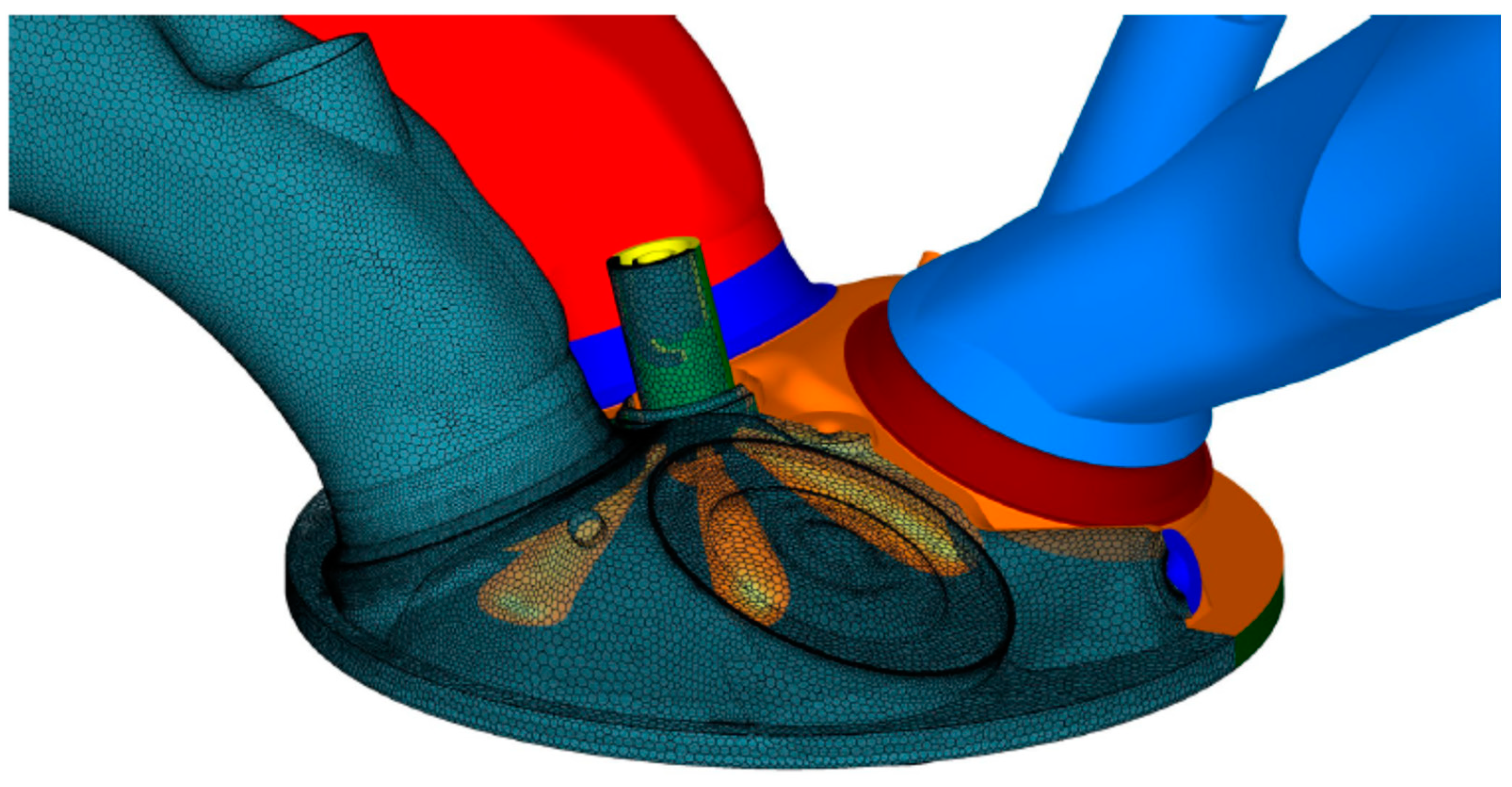
The 3D-CFD of AVL gives the first element [29] dedicated to the modeling, simulations, and calculus of internal combustion engine phenomena, starting from the initial air intake and finishing at the burn gas flow exhaust, computing all the velocities and temperatures of the gas flow through all the internal duct elements.

-

The second element is given by using all the values of the velocities and temperatures of the gas flow through the final muffler gas exhaust in the classic TMM to compute the TL of the AEM, which has a specific geometry and structure.

The first element of MTMM consists of a 3D-CFD AVL FIRE^TM M Engine [29] based on the following steps: good reproduction of realistic geometry by discretization, physically feasible boundary conditions, operating conditions applied to the model given by boundary conditions, and the best-suited physical models.

The second element of MTMM is the classic TMM, which is used to compute the TL of a specific AEM using the data already determined with 3D-CFD AVL FIRE^TM M Engine, respectively, the velocities and temperatures of the gas flow through the muffler.

For plane wave propagation in a rigid straight pipe of length L, constant cross-section S, and transporting a turbulent incompressible mean flow of velocity V (see Figure 1), the sound pressure p and the volume velocity v anywhere in the pipe element can be represented as the sum of left and right traveling waves. The plane wave propagation model is valid when the influence of higher-order modes can be neglected. Using the impedance analogy, the sound pressure p and volume velocity ν at positions 1 (upstream end) and 2 (downstream end), as in Figure 1 (x = 0 and x = L, respectively), can be expressed by the following equations

$$p_1=A{p}_2+B{\nu }_2,$$

(1)

$${\nu }_1=C{p}_2+D{\nu }_2,$$

(2)

where A, B, C, and D are called the four-pole constants.

The four-pole constants for the non-viscous medium are expressed, as in [1], in the following mathematical form:

$$A=\exp (-jM{k}_{c}L)\cos k_{c}L,$$

(3)

$$B=j(\rho c/S)\exp (-jM{k}_{c}L)\sin k_{c}L,$$

(4)

$$D=\exp (-jM{k}_{c}L)\cos k_{c}L,$$

(5)

$$C=j(S/\rho c)\exp (-jM{k}_{c}L)\sin k_{c}L,$$

(6)

$$j=\sqrt{-1},M=\frac{V}{c},k=\frac{2\pi f}{c},k_c=\frac{k}{1-M^2},$$

(7)

where M is the Mach number, f is the sound frequency, c is the sound speed, $\rho$ is the fluid density, S is the cross-section area, and L is the length. Equations (1) and (2) can be put into the following matrix form:

$$\left[\begin{array}{c}{p}_1\\ {\upsilon }_1\end{array}\right]=\left[\begin{array}{cc}A& B\\ C& D\end{array}\right]\left[\begin{array}{c}{p}_2\\ {\upsilon }_2\end{array}\right],$$

(8)

where the second matrix relates the total sound pressure and volume velocity at two points in a muffler element, such as the straight pipe discussed in the previous section; thus, a transfer matrix is a frequency-dependent property of the system. The reciprocity principle requires that the transfer matrix determinant be 1. In addition, A and D must be identical for a symmetrical muffler. In practice, different elements, such as a perforated tube, are connected in an actual muffler, as shown in Figure 2. However, the four-pole constant values of each component are not affected by connections to elements upstream or downstream if the system elements can be assumed to be linear and passive. So, each element is characterized by one transfer matrix that depends on its geometry and flow conditions. Therefore, it is necessary to model each element and then relate all of them to obtain the overall acoustic property of the muffler.

Suppose several muffler elements, such as sudden expansions, contractions, extended tubes, and perforated tubes, are connected in series. In that case, the overall transfer matrix of the entire system is given by the product of the individual system matrix. For example, the muffler shown in Figure 2 includes an extended straight tube (1 in Figure 2), sudden expansion (2 in Figure 2) and extended inlet (3 in Figure 2), uniform tube, sudden contraction (4 in Figure 2), concentric resonator with a perforated pipe (5 in Figure 2), and a straight tailpipe (6 in Figure 2). All the blocks presented in Figure 2 are designed to increase the global TL of the muffler. Then, for this muffler, the total transfer matrix of the system is

$$T=T_1{T}_2{T}_3{T}_4{T}_5{T}_6.$$

(9)

For continuous cross-sections, such as extended tubes, the transfer matrix has the form

$$T_i=e^{-j{M}_i{k}_c{l}_i}\left[\begin{array}{cc}\cos (k{l}_i)& j{Y}_i\sin (k{l}_i)\\ \frac{j}{Y_i}\sin (k{l}_i)& \cos (k{l}_i)\end{array}\right],Y_i=\frac{c}{S_i},$$

(10)

while for discontinuity cross-sections, such as sudden contraction or expansion, the transfer matrix has the form

$$T_i=\left[\begin{array}{cc}1& 0\\ \frac{j}{Y_{i}ctg(k{l}_i)}& 1\end{array}\right],Y_i=\frac{c}{S_i-S_{i-1}},M_i=0.$$

(11)

When $M_i\ne 0.$ the computation of the transfer matrix is more complex based on the parameter elements of the transition section up-stream and down-stream flux, considering the equation of continuity [30]:

$$C_1{S}_1+C_2{S}_2+S_3=0,$$

(12)

where the constants $C_1$ and $C_2$ (see

Table 1. Parameter values of the transition elements for discontinuity [30].

Element Type	${\mathit{C}}_1$	${\mathit{C}}_2$	$\mathit{K}$
	−1	−1	$\frac{\left(1-\frac{S_1}{S_3}\right)}{2}$
	−1	1	${\left(\frac{S_1}{S_3}-1\right)}^2$
	1	−1	${\left(\frac{S_1}{S_3}\right)}^2$
	1	−1	−0.5

) are selected to satisfy the mass conservation equation across the transition.

For an AEM, as illustrated in Figure 3, the general scheme is presented in Figure 4, representing a triple-chamber muffler with perforations. The blocks mentioned in Figure 4 represent the following parts: 1—inlet straight tube; 2 and 8—sudden expansions (2 and 8 in Figure 4, discontinuities); 3—extended inlet (3 in Figure 4); 4 and 10—discontinuities as sudden contractions; 11—outlet straight tube; 9—constant inlet; 6—resonator with multiple perforations (discontinuity); 5 and 7—part of the discontinuities of 4 and 8 of the inlet duct.

The 6th region of the muffler presented in Figure 4 is illustrated in detail in Figure 5. For the triple-chamber muffler shown in Figure 4, the continuous regions are 1, 3, 9, and 11, and their transfer matrices are expressed in the mathematical matrix relations.

$$\begin{array}{l}{T}_1=e^{-j{M}_1{k}_c{l}_1}\left[\begin{array}{cc}\cos (k{l}_1)& j{Y}_1\sin (k{l}_1)\\ \frac{j}{Y_1}\sin (k{l}_1)& \cos (k{l}_1)\end{array}\right],T_3=e^{-j{M}_3{k}_c{l}_3}\left[\begin{array}{cc}\cos (k{l}_3)& j{Y}_3\sin (k{l}_3)\\ \frac{j}{Y_3}\sin (k{l}_3)& \cos (k{l}_3)\end{array}\right],\\ T_9=e^{-j{M}_9{k}_c{l}_9}\left[\begin{array}{cc}\cos (k{l}_9)& j{Y}_9\sin (k{l}_9)\\ \frac{j}{Y_9}\sin (k{l}_9)& \cos (k{l}_9)\end{array}\right],T_{11}=e^{-j{M}_{11}{k}_c{l}_{11}}\left[\begin{array}{cc}\cos (k{l}_{11})& j{Y}_{11}\sin (k{l}_{11})\\ \frac{j}{Y_{11}}\sin (k{l}_{11})& \cos (k{l}_{11})\end{array}\right],\\ Y_1=\frac{c}{S_1},Y_3=\frac{c}{S_3},Y_9=\frac{c}{S_9},Y_{11}=\frac{c}{S_{11}},c=c_0\sqrt{1+\frac{t_1}{273}},\\ M_1=\frac{V_1}{c_0\sqrt{1+\frac{t_1}{273}}},M_3=\frac{V_3}{c_0\sqrt{1+\frac{t_3}{273}}},M_9=\frac{V_9}{c_0\sqrt{1+\frac{t_9}{273}}},M_{11}=\frac{V_{11}}{c_0\sqrt{1+\frac{t_{11}}{273}}},\end{array}$$

(13)

where the mean gas flow velocities $V_i,i=1,3,9,11$ are computed based on the mass conservation Equation (12) across the transition; the temperatures $t_i,i=1,3,9,11$ are calculated for each region considering an adiabatic flow of the burn gases through the muffler; and $c_0$ is the sound speed at standard temperature ($T_0=273K,p_0=0.1013MPa$). The blocks illustrated in Figure 5 have the same significance as those mentioned in Figure 4, where Figure 5 provides details for the elements 4–8 in Figure 4. For the discontinuity regions 2, 4, 8, and 10 (see Figure 4), the transfer matrices are expressed in the mathematical matrix form.

$$T_2=\left[\begin{array}{cc}1& K_2{M}_3{Y}_3\\ \frac{1}{M_1{Y}_1-Z_2}& \frac{S_2{Z}_2-M_3{Y}_3\left(S_1{K}_2-S_3\right)}{S_2{Z}_2+S_1{M}_1{Y}_1}\end{array}\right],K_2={\left(\frac{S_3}{S_1}-1\right)}^2,Z_2=-j{Y}_{2}ctg\left(k{l}_2\right),M_i=\frac{V_i}{c_0\sqrt{1+\frac{t_i}{273}}},Y_i=\frac{c_0\sqrt{1+\frac{t_i}{273}}}{S_i},i=1,3,$$

(14)

$$T_4=\left[\begin{array}{cc}1& K_4{M}_5{Y}_5\\ \frac{1}{Z_4-M_3{Y}_3}& \frac{S_4{Z}_4+M_5{Y}_5\left(S_3{K}_4-S_5\right)}{S_4{Z}_4-S_3{M}_3{Y}_3}\end{array}\right],K_4=\left(0.5-0.5\frac{S_5}{S_3}\right),Z_4=-j{Y}_{4}ctg\left(k{l}_4\right),M_i=\frac{V_i}{c_0\sqrt{1+\frac{t_i}{273}}},Y_i=\frac{c_0\sqrt{1+\frac{t_i}{273}}}{S_i},i=3,5,$$

(15)

$$T_8=\left[\begin{array}{cc}1& K_8{M}_9{Y}_9\\ \frac{1}{M_7{Y}_7-Z_8}& \frac{S_8{Z}_8-M_9{Y}_9\left(S_7{K}_8-S_9\right)}{S_8{Z}_8+S_7{M}_7{Y}_7}\end{array}\right],K_8={\left(\frac{S_9}{S_7}-1\right)}^2,Z_8=-j{Y}_{8}ctg\left(k{l}_8\right),M_i=\frac{V_i}{c_0\sqrt{1+\frac{t_i}{273}}},Y_i=\frac{c_0\sqrt{1+\frac{t_i}{273}}}{S_i},i=7,9,$$

(16)

$$T_{10}=\left[\begin{array}{cc}1& K_{10}{M}_{11}{Y}_{11}\\ \frac{1}{Z_{10}-M_9{Y}_9}& \frac{S_{10}{Z}_{10}+M_{11}{Y}_{11}\left(S_9{K}_{10}-S_{11}\right)}{S_{10}{Z}_{10}-S_9{M}_9{Y}_9}\end{array}\right],K_{10}=\left(0.5-0.5\frac{S_{11}}{S_9}\right),Z_{10}=-j{Y}_{10}ctg\left(k{l}_{10}\right),M_i=\frac{V_i}{c_0\sqrt{1+\frac{t_i}{273}}},Y_i=\frac{c_0\sqrt{1+\frac{t_i}{273}}}{S_i},i=9,11.$$

(17)

The 6th region of the muffler, presented in Figure 4, represents a resonator composed of two concentrical ducts of cross-section area $S_{6e},S_{6i}$ (one external, one internal); the inner flow duct has the lengths $l_{6in},l_{6p},l_{6out},$ $l_6=l_{6in}+l_{6p}+l_{6out}$, where $l_{6p}$ is the length with perforations, and $l_{6in},l_{6out},$ are the lengths without perforations. The transfer matrix for this discontinuity is computed as for a concentric-tube resonator [5]. Such a resonator has the geometry of the perforations illustrated in Figure 6, where C is the distance between perforations and $d_h$ is the diameter of a perforation, yielding, as in [5], the relations.

$$\begin{array}{l}{T}_6=\left[\begin{array}{cc}1& 0\\ \frac{1}{Z_{6r}}& 1\end{array}\right],Z_{6r}=Z_{6p}+Z_{6c},\\ Z_{6p}=\frac{Y_{6p}}{\sigma }\left[0.0073\left(1+72M_6\right)+0.000022j\left(1+51t_{6p}\right)\left(1+204d_h\right)f\right],\\ Z_{6c}=-j{Y}_{6c}\frac{1}{tg\left(k{l}_{6in}\right)+tg\left(k{l}_{6out}\right)},Y_{6p}=\frac{c_0\sqrt{1+\frac{t_6}{273}}}{S_{6p}},Y_{6c}=\frac{c_0\sqrt{1+\frac{t_6}{273}}}{S_{6c}},\\ M_6=\frac{V_6}{c_0\sqrt{1+\frac{t_6}{273}}},S_{6p}=0.25d_h^2,S_{6c}=S_{6e}-S_{6i},\sigma =\frac{S_{6p}}{C^2},\end{array}$$

(18)

where $Z_{6r}$ is the concentric-tube resonator; $Z_{6p}$ is the acoustic impedance generated by the perforations; $Z_{6c}$ is the acoustic cavity resonance; $\sigma$ is the porosity of the perforated area; $t_{6p}$ is the thickness of the perforated tube; C is the distance between perforations; and $d_h$ is the diameter of a perforation.

The global transfer matric for the automotive’s exhaust muffler (AME), considering the relations (9), (13)–(18) is

$$T{L}_{AME}=\left[\begin{array}{cc}{T}_{11}& T_{12}\\ T_{21}& T_{22}\end{array}\right]={\displaystyle \prod _{i=1}^{11}{T}_i},$$

(19)

thus yielding the $T{L}_{AME}$ for this special acoustic muffler with triple-chamber and perforations

$$T{L}_{AME}=20\log \left[{\left(\frac{Y_{11}}{Y_1}\right)}^{0.5}\left|0.5\left(T_{11}+\frac{T_{12}}{Y_{11}}+T_{21}{Y}_1+T_{22}\frac{Y_1}{Y_{11}}\right)\right|\right].$$

(20)

Using Equations (13)–(20), the transmission loss of an AME was computed using, as a first step of computations, 3D-CFD AVL FIRE^TM M Engine to calculate the Mach numbers, the mean gas flow velocities, and the temperatures for each element of the muffler exhaust. After this stage, these values were inserted into relations of the classic TMM expressed by the abovementioned Equations (13)–(20) to determine the TL for the AME.

3. Results and Discussions

Based on Equations (13)–(20), we used MATLAB Software to compute the transmission loss of an automotive muffler exhaust $T{L}_{AME}$ for the muffler having a triple-chamber with perforations (see Figure 4), designed for an automotive having a standard engine of 90 kW. Based on specialized software for engines 1D-CFD (computation fluid dynamics in 1D), presented and developed in [31] (pp. 44–184, 240–290), the speed flow of the exhaust gases entering the muffler was calculated for an internal combustion engine of an Audi 1.4 TSI having the power 90 kW, with values in the range $V_1\in \left[60.0–102.0\right]$ m/s and the temperature of the exhaust gases at the muffler in the range $t_1\in \left[60.0,135.0\right]$ °C. The geometric characteristics of the muffler are presented in

Table 2. The dimensions considered in the first stage of computation.

${\mathit{S}}_1$ [m2]	${\mathit{S}}_3$ [m2]	${\mathit{l}}_1$ [mm]	${\mathit{l}}_2$ [mm]	${\mathit{l}}_3$ [mm]	${\mathit{l}}_4$ [mm]	${\mathit{l}}_{6\mathit{i}\mathit{n}}$ [mm]	${\mathit{l}}_{6\mathit{p}}$ [mm]	${\mathit{l}}_7$ [mm]	${\mathit{d}}_{\mathit{h}}$ [mm]	C [mm]
0.003318	0.031416	80	45	120	50	65	50	50	3	10

, knowing that $S_1=S_5=S_{6i}=S_7=S_{11},$ $S_3=S_{6e}=S_9,$ $l_1=l_{11},$ $l_2=l_{10},$ $l_3=l_9,$ $l_4=l_5,$ $l_{6in}=l_{6out},$ $l_7=l_8$ from geometric construction. Based on the dimensions in Table 2, Figure 7 illustrates the technical drawing of the muffler exhaust.

Figure 8, Figure 9, Figure 10 and Figure 11 illustrate the transmission loss of an automotive muffler exhaust $T{L}_{AME}$ in the frequency range [10, 4500] Hz. For different engine rotation speeds, states are characterized by different values of the speed flow of the exhaust gases and other values of the temperature of the exhaust gases at the mufflers in the previously mentioned ranges.

Figure 8 illustrates the results of the transmission loss of an automotive muffler exhaust $T{L}_{AME}$ in the frequency range [10, 4500] Hz, disregarding the exhaust gases’ temperature for the value of the speed flow of the exhaust gases $V_1=68$ m/s. Comparing these data with those illustrated in Figure 9 for the temperature of the exhaust gases $t_1=60$ °C, it can be determined that the minimum of the transmission loss of an automotive muffler exhaust $T{L}_{AME}$ is manifested at the frequency of 1957 Hz compared with the previously 1890 Hz. Also, this transmission loss value is slightly different from 7.276 dB to 7.296 dB. Thus, it can be concluded that the temperature of the exhaust gases influences the frequency range and the transmission loss values in the modified TMM algorithm.

Figure 10 and Figure 11 illustrate the results of the transmission loss of an automotive muffler exhaust $T{L}_{AME}$ in the frequency range [10, 4500] Hz for the speed flow of the exhaust gases $V_1=86$ m/s and $V_1=96$ m/s, whereby the corresponding temperatures of the exhaust gases are $t_1=80$ °C and $t_1=120$ °C, respectively. It can be remarked, upon analyzing these figures, that the increase in the speed flow of the exhaust gases and the increase in the temperature of the exhaust gases induce a boost for the frequency’s value, which reaches the minimum value of the $T{L}_{AME}$.

The results obtained and illustrated in Figure 8, Figure 9, Figure 10 and Figure 11 are compared with data published in the literature [32], and agreement was found in the frequency range 1800-2500 Hz.

Based on the 3D-CFD AVL FIRE^TM M Engine, it was computed, for the same internal combustion engine of Audi 1.4 TSI with a power of 90 kW, the velocity flow of the exhaust gases entering the AEM (see Figure 7) and the velocities in all the continuity and discontinuity sections of the AEM, as well as the temperature at the AEM’s intake and the temperatures in all the continuity and discontinuity sections of the AEM. Figure 12 illustrates the 3D discretization of the exhaust tailpipe and the cylinder head of the internal combustion engine used by the software AVL FIRE^TM M Engine to compute the exhaust velocities and the exhaust temperatures of the flow gas.

Based on the input data values for the flow velocities and the temperatures of the flowing gas through the AEM and the MATLAB software, which were built on Equations (13)–(20) to compute the $T{L}_{AME}$ in the frequency range [0.1, 4.5] kHz, the results for the exhaust muffler illustrated in Figure 7 (geometry details are presented in Table 2) are further illustrated in Figure 13, Figure 14, Figure 15 and Figure 16.

Compared with Figure 8, Figure 9, Figure 10 and Figure 11, Figure 13, Figure 14, Figure 15 and Figure 16 illustrate the results of $T{L}_{AME}$ at different engine rotation speeds n for the internal combustion engine of Audi 1.4 TSI with 90 kW of power.

Analyzing the results presented in Figure 13, Figure 14, Figure 15 and Figure 16, it can be remarked that increasing the engine rotation speed in the range 1500–4500 rpm decreases the mean value of the $T{L}_{AME}$ by 10 dB in the frequency range 100–1400 Hz; by 14 dB in the frequency range 1500–2500 Hz; and by 12 dB in the frequency range 2500–4000 Hz. The results obtained and illustrated in Figure 13, Figure 14, Figure 15 and Figure 16 are compared with data published in the literature [33], and agreement was found in the 100-4000 Hz frequency range.

An important conclusion of this study is that using the 3D-CFD AVL FIRE^TM M Engine before using the classic TMM to compute the $T{L}_{AME}$ instead of 1D-CFD, presented and developed in [31] (pp. 44–184, 240–290), enlarges the frequency range from 1800–2500 Hz to 100–4000 Hz for the MTMM. A limitation of this study, however, which uses this final MTMM (3D-CFD AVL FIRE^TM M Engine linked with the classic TMM) to compute the $T{L}_{AME}$, is the frequency range 100-4000 Hz, as this is a disadvantage. It is particularly needed to accurately predict the $T{L}_{AME}$ in the frequency range 100-8000 Hz. Concerning the accuracy of $T{L}_{AME}$ predicted with the MTMM, compared with the accuracy of the data published in the literature [33], several aspects of the data predicted and illustrated in Figure 13, Figure 14, Figure 15 and Figure 16 are noted:

-

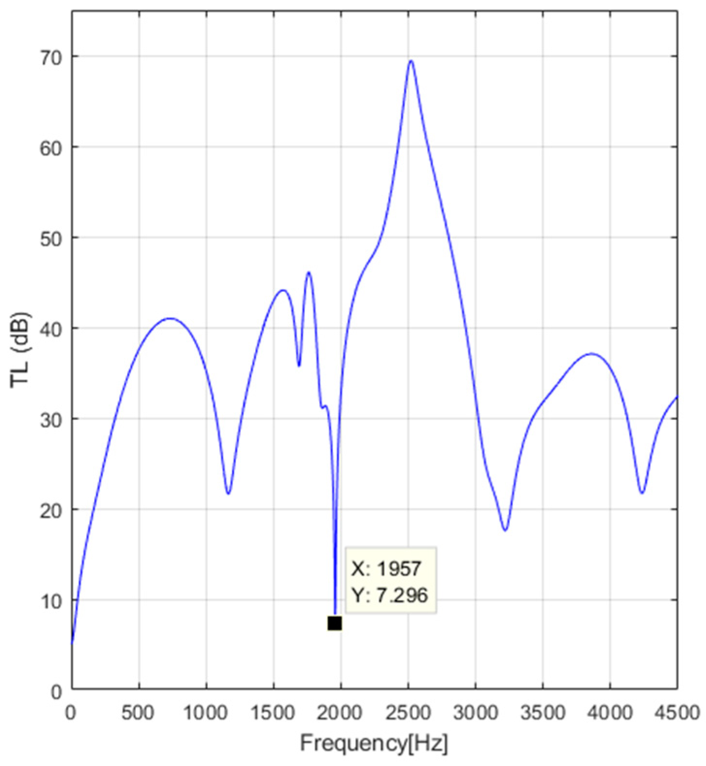
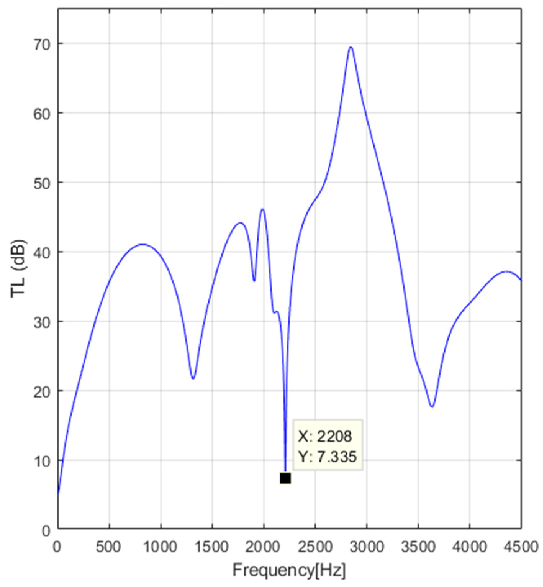
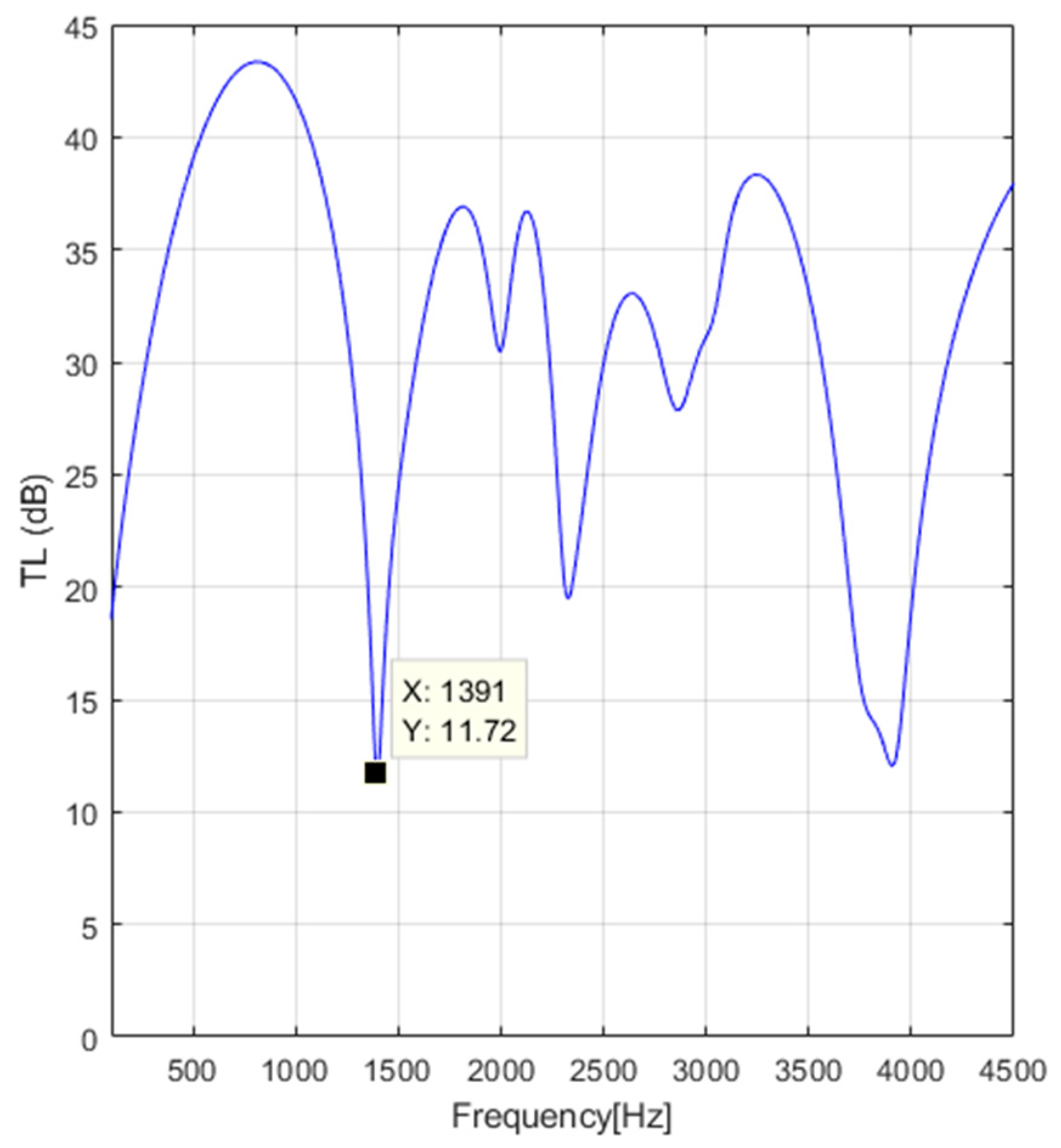
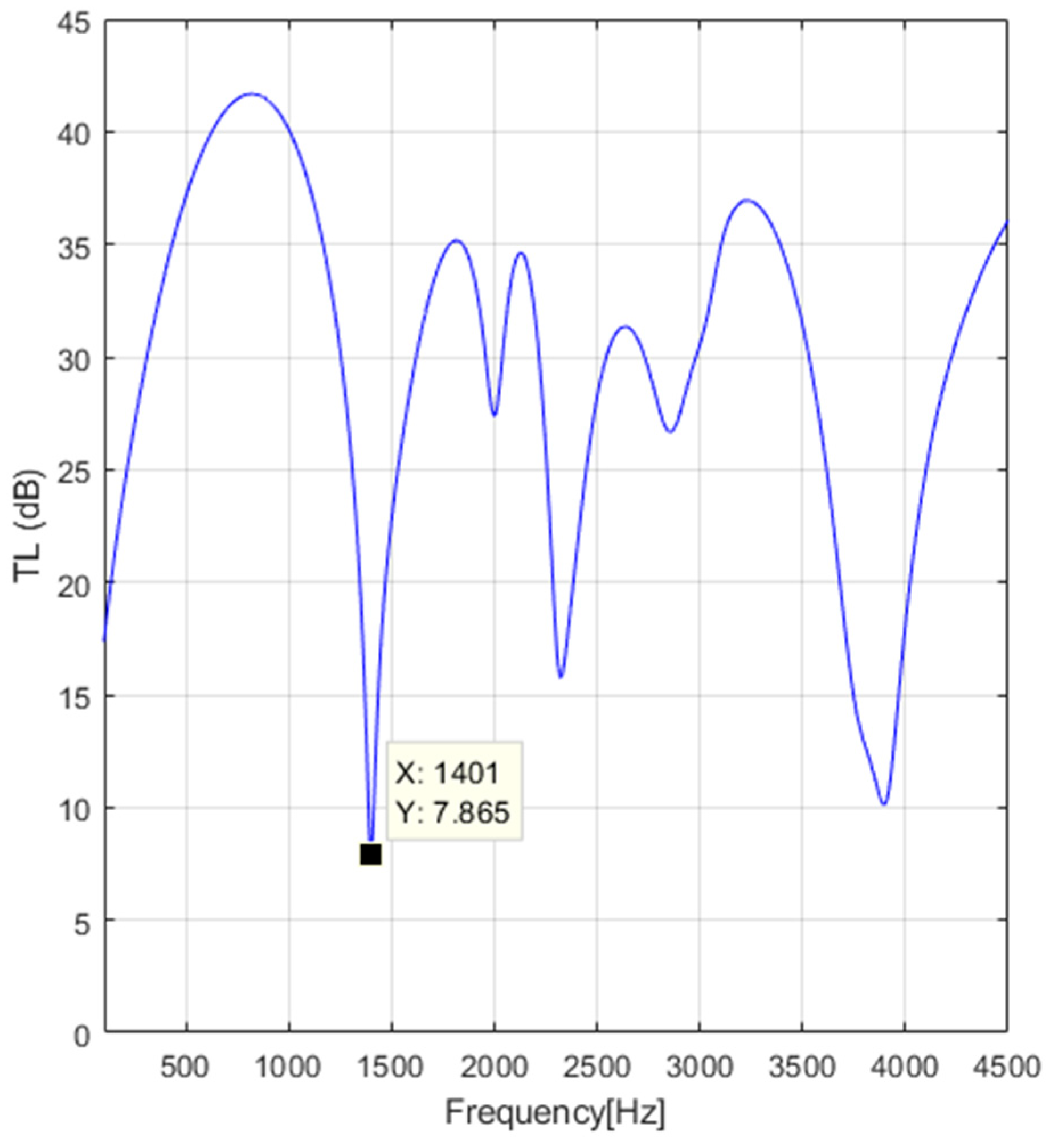
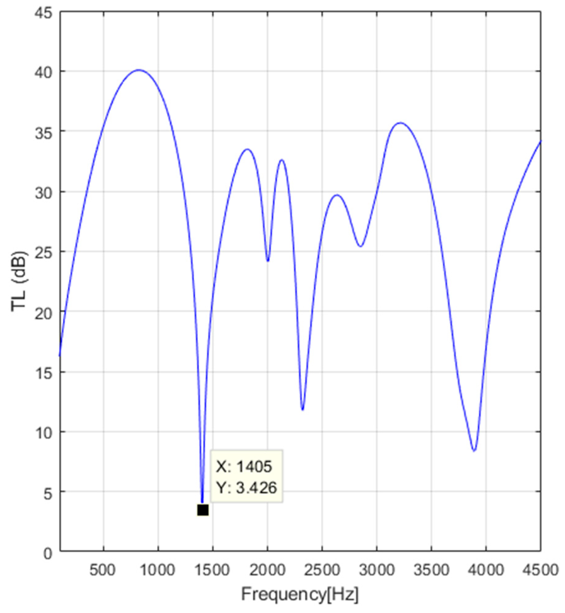
In the frequency range 0.1–4.0 kHz and for engine rotation speeds in the range 1500–2500 rpm, the predicted values of $T{L}_{AME}$ are 1–4% higher than the experimental ones mentioned in [33], while for engine rotation speeds in the range, 3500–4500 rpm, the predicted values are 4.5–8% higher than the experimental ones mentioned in [33].

-

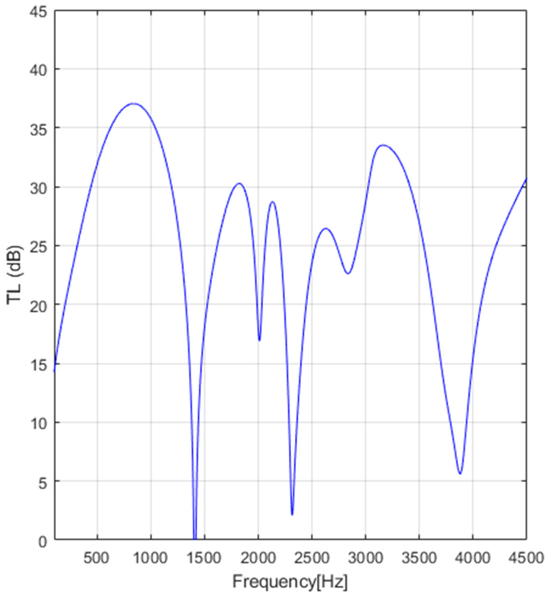
For the frequency range over 4.0 kHz for engine rotation speeds in the range 1500-4500 rpm, the predicted values are at least 11% larger or even smaller by 14% than the experimental ones mentioned in [33].

4. Conclusions

The present work aims to investigate the employment of the new MTMM, based on the dedicated FEM 3D-CFD AVL FIRE^TM M Engine, to calculate in detail the velocities of gas flow and the temperatures of the gas flow in all the process phenomena of the internal combustion engine from the air intake to the gas exhaust through the AEM, coupled with the classic TMM for the AEM, to predict the $T{L}_{AME}$. For all the continuous and discontinuous sections of the AEM, the Mach number of the cross-section, the temperature, and the type of discontinuity of the exhaust gas flow were considered to evaluate the specific elements of the acoustic quadrupole that define the MTMM. The perforations of intermediary ducts were considered in the new MTMM to predict the TL of an automotive exhaust muffler with three expansion chambers. The flow chart of the MTMM consists of the following:

• The use of 3D-CFD AVL FIRE^TM M Engine (based on FEM in 3D) to calculate the gas flow velocities and the gas flow temperatures of all the internal ducts of the internal combustion engine (taken into consideration, respectively, the internal combustion engine of Audi 1.4 TSI with a power of 90 kW) in all the process phenomena, from the initial air intake through the air filter to the cylinders, compression, ignition, detention, and burnt gas exhaust, from the cylinders to the exhaust manifold, gas flow through the catalytic muffler, and the exhaust through the AME.
• The use of the data results for the gas flow velocities and the gas flow temperatures obtained using 3D-CFD AVL FIRE^TM M Engine in the classic TMM for the given AEM (see Figure 13, Figure 14, Figure 15 and Figure 16) to compute $T{L}_{AME}$.

The most important conclusion of the present study is that using the 3D-CFD AVL FIRE^TM M Engine before using the classic TMM to compute the $T{L}_{AME}$ instead of 1D-CFD, presented and developed in [31] (pp. 44–184, 240–290), enlarges the frequency range from 1800–2500 Hz to 100–4000 Hz for the MTMM.

From the results of the predicted data for the $T{L}_{AME}$, another conclusion is evident: the new MTMM is sensitive to the temperature of the exhaust gases and to the engine rotation speed n. The results obtained in the frequency range 0.1–4.0 kHz agree with the experimental results published in the literature [32,33]. In this way, the MTMM was improved as a valuable tool in designing the automotive exhaust muffler based on the 3D-CFD AVL FIRE^TM M Engine.

The MTMM must also be developed for the reverse-flow discontinuity elements of the AME (the present study deals with the cross-flow discontinuity elements of the AME), extending in the meantime the frequency range to 0.1–8.0 kHz to predict the $T{L}_{AME}$ accurately.

References

1. Bugaru, M.; Enescu, N. An overview of muffler modeling by transfer matrix method. Sci. Bull. Politeh. Univ. Timis. Trans. Mech. 2005, 1, 51–54. [Google Scholar]
2. Chung, J.Y.; Blaser, D.A. Transfer function method of measuring in-duct acoustic properties: I. Theory and II. Experiment. J. Acoust. Soc. Am. 1980, 68, 907–921. [Google Scholar] [CrossRef]
3. Davies, P.O.A.L. Realistic models for predicting sound propagation in flow duct systems. Noise Control Eng. J. 1993, 40, 135–141. [Google Scholar] [CrossRef]
4. Mechel, F.P. Formulas of Acoustics; Springer: Berlin/Heidelberg, Germany, 2002. [Google Scholar]
5. Munjal, M.L. Acoustics of Ducts and Mufflers, 1st ed.; John Wiley and Sons: New York, NY, USA, 1987. [Google Scholar]
6. Sridhara, B.S.; Crocker, M.J. Review of theoretical and experimental aspects of acoustical modeling of engine exhaust systems. J. Acoust. Soc. Am. 1994, 95, 2363–2370. [Google Scholar] [CrossRef]
7. Kumar, S. Linear Acoustic Modelling and Testing of Exhaust Muffler. Master’s Thesis, The Royal Institute of Technology, Stockholm, Sweden, January 2007. Available online: https://www.google.com/url?sa=t&rct=j&q=&esrc=s&source=web&cd=&ved=2ahUKEwik7fSMv6CEAxXH_7sIHauBCwgQFnoECBUQAQ&url=https%3A%2F%2Fwww.diva-portal.org%2Fsmash%2Fget%2Fdiva2%3A11878%2FFULLTEXT01.pdf&usg=AOvVaw36bDa-Lk1NGDXCyrbz8u9R&opi=89978449 (accessed on 10 February 2024).
8. Pal, S. Design and Acoustic Analysis of Exhaust Mufflers for Automotive Applications. Master’s Thesis, Christ University, Bengaluru, India, March 2015. Available online: https://www.researchgate.net/publication/275408198 (accessed on 10 February 2024).
9. Yasuda, T.; Wu, C.; Nakagawa, N.; Nagamura, K. Predictions and experimental studies of the tail pipe noise of an automotive muffler using a one dimensional CFD model. Appl. Acoust. 2010, 71, 701–707. [Google Scholar] [CrossRef]
10. Suwandi, D.; Middelberg, J.; Byrne, K.P.; Kessissoglou, N.J. Predicting the Acoustic Performance of Mufflers using Transmission Line Theory. In Proceedings of the ACOUSTICS 2005, Busselton, Australia, 9–11 November 2005; pp. 181–187. [Google Scholar] [CrossRef]
11. Kalita, U.; Singh, M. Prediction of Transmission Loss on a Simple Expansion Chamber Muffler. J. Emerg. Technol. Innov. Res. 2018, 5, 1022–1031. Available online: https://www.researchgate.net/publication/347950563 (accessed on 10 February 2024).
12. Mohammad, M.; Muhamad, S.M.F.; Khairudin, M.H.; Kadir, M.K.; Dahlan, M.A.A.; Zaw, T. Complex geometry automotive muffler sound transmission loss measurement by experimental method and 1 D simulation correlation. In Proceedings of the Sustainable and Integrated Engineering International Conference SIE 2019, Putrajaya, Malaysia, 8–9 December 2019; p. 012098. [Google Scholar] [CrossRef]
13. Olgar, T. Acoustical Analysis of Exhaust Mufflers for Earth-Moving Machinery. Master’s Thesis, Middle East Technical University, Ankara, Turkey, September 2009. Available online: https://open.metu.edu.tr/handle/11511/19024 (accessed on 10 February 2024).
14. Fu, J.; Xu, M.; Zhang, Z.; Kang, W.; He, Y. Muffler structure improvement based on acoustic finite element analysis. J. Low Freq. Noise Vib. Act. Control 2019, 18, 415–416. [Google Scholar] [CrossRef]
15. Zhang, L.; Shi, H.M.; Zeng, X.H.; Zhuang, Z. Theoretical and Experimental Study on the Transmission Loss of a Side Outlet Muffler. Hindawi Schock Vib. 2020, 2020, 6927574. [Google Scholar] [CrossRef]
16. Patne, M.M.; Sentilkumar, S.; Stanley, J.M. Numerical Analysis on Improving Transmission Loss of Reactive Muffler using Various Sound Absorptive Materials. In Proceedings of the ICMECE 2020, Knacheepuram, India, 22 April 2020; Volume 993, p. 012150. [Google Scholar] [CrossRef]
17. Fan, W.; Guo, L.-X. An Investigation of Acoustic Attenuation Performance of Silencers with Mean Flow Based on Three-Dimensional Numerical Simulation. Hindawi Schock Vib. 2016, 2016, 6797593. [Google Scholar] [CrossRef]
18. Puthuparampil, J.X. Aeroacoustic Noise Prediction and Acoustic Optimization of Mufflers. Master’s Thesis, University of Toronto, Toronto, ON, Canada, November 2018. Available online: https://tspace.library.utoronto.ca/handle/1807/91618 (accessed on 10 February 2024).
19. Xie, X. Noise optimization design on the exhaust muffler of a special vehicle on the improved genetic algorithm. J. Vibroengineering 2015, 17, 4625–4639. Available online: https://www.semanticscholar.org/paper/Noise-optimization-design-on-the-exhaust-muffler-of-Xie/f338124725c16ed33bf4774e4d4cebbd42d11a3c#citing-papers (accessed on 10 February 2024).
20. Bowden, D.R. Development of a large experimental acoustic transmission loss test bench suitable for large marine diesel exhaust system components. In Proceedings of the ACOUSTICS 2016, Brisbane, Australia, 9–11 November 2016; Available online: https://www.google.com/url?sa=t&rct=j&q=&esrc=s&source=web&cd=&ved=2ahUKEwjO_eCB_KKEAxW2_rsIHYCxBioQFnoECA0QAQ&url=https%3A%2F%2Facoustics.asn.au%2Fconference_proceedings%2FAASNZ2016%2Fpapers%2Fp54.pdf&usg=AOvVaw0YkzRvANLZayLyaMfRf_Uh&opi=89978449 (accessed on 10 February 2024).
21. Mohamad, B. A review of flow acoustic effects on a commercial automotive exhaust system-methods and materials. J. Mech. Energy Eng. 2019, 3, 149–156. [Google Scholar] [CrossRef]
22. Babu, S.; Akhildev, V.P.; Sabu, J. Design optimization of hybrid muffler and acoustic transmission loss prediction. Int. Res. J. Eng. Technol. 2020, 7, 2721–2727. Available online: https://www.google.com/url?sa=t&rct=j&q=&esrc=s&source=web&cd=&ved=2ahUKEwiahqyrhaOEAxWn7rsIHTeYCJcQFnoECA8QAQ&url=https%3A%2F%2Fwww.irjet.net%2Farchives%2FV7%2Fi7%2FIRJET-V7I7482.pdf&usg=AOvVaw1ApSTc3ld9e3kSk79k_cLH&opi=89978449 (accessed on 10 February 2024).
23. Liu, L.; Zheng, X.; Hao, Z.; Qiu, Y. A time-domain simulation method to predict insertion loss of a dissipative muffler with exhaust flow. Phys. Fluids 2021, 33, 067114. [Google Scholar] [CrossRef]
24. Damyar, N.; Mansouri, F.; Khavanin, A.; Jafari, A.J.; Asilian-Mahabadi, H.; Mirzaei, R. Acoustical Performance of a Double-Expansion Chamber Muffler: Design and Evaluation. Health Scope 2022, 11, e103226. [Google Scholar] [CrossRef]
25. Das, S.; Das, S.; Mondal, K.; Ahmad, A.; Shuayb, S.A.; Faizan, M.; Ameen, S.; Pandey, A.; Vadiraja, B.R. A novel design for muffler chambers by incorporating baffle plate. Appl. Acoust. 2022, 197, 108888. [Google Scholar] [CrossRef]
26. Cheng, Y.; Yuan, W.; Fu, J.; Ma, Y.; Zheng, W. Research on the Influence of Characteristics of the Annular Connecting Pipe, on the Transmission Loss of the Expanded Exhaust Muffler. Hindawi Schock Vib. 2024, 2024, 3404328. [Google Scholar] [CrossRef]
27. Cui, Z.; Huang, Y. Boundary Element Analysis of Muffler Transmission Loss With LS-DYNA. In Proceedings of the LS-DYNA 12th International Conference, Detroit, MI, USA, 3–5 June 2012; Available online: https://www.dynamore.de/en/training/conferences/past/12.-internationale-ls-dyna-konferenz (accessed on 18 March 2024).
28. Vasile, O. Theoretical and experimental analysis of acoustic performances on the multi-chamber muffler. In Proceedings of the 21st International Congress on Sound and Vibration, Beijing, China, 13–17 July 2014; Available online: https://www.academia.edu/94861050/Theoretical_and_Experimental_Analysis_of_Acoustic_Performances_on_the_Multi_Chamber_Muffler?uc-g-sw=30082541 (accessed on 18 March 2024).
29. AVL FIRETM M Engine. Available online: https://www.avl.com/en/engineering/vehicle-engineering/vehicle-systems-development-and-integration (accessed on 18 March 2024).
30. Beranek, L.L.; Istvan, L. Noise and Vibration Control Engineering: Principles and Applications; John Wiley & Sons: New York, NY, USA, 1992. [Google Scholar]
31. Grünwald, B. Theory, Computation and Design of Internal Combustion Engines for Automotive; Didactic & Pedagogical Publishing House: Bucharest, Romania, 1980. (In Romanian) [Google Scholar]
32. Abdul Rani, M.N.; Mat Isa, A.A.; Rahman, Z.A.; Ali Al-Assadi, H.M.A. Dynamic characterization of an exhaust system. J. Mech. Eng. 2011, 8, 41–55. Available online: https://www.researchgate.net/publication/289188425_Dynamic_characterisation_of_an_exhaust_system (accessed on 10 February 2024).
33. Tao, Z.; Seybert, A.F. A review of current techniques for measuring muffler Transmission Loss. SAE Trans. 2003, 112, 2096–2100. Available online: https://www.jstor.org/stable/44745590 (accessed on 19 March 2024).
Figure 1. Plane wave propagation [1].
Computation 12 00073 g001
Figure 2. Real muffler [1].
Computation 12 00073 g002
Figure 3. Actual triple-chamber muffler with central perforations.
Computation 12 00073 g003
Figure 4. Triple-chamber muffler with perforations [1].
Computation 12 00073 g004
Figure 5. The 6th region of the muffler of the triple-chamber muffler with perforations [1].
Computation 12 00073 g005
Figure 6. Geometry of the perforations [1].
Computation 12 00073 g006
Figure 7. The technical drawing of the muffler exhaust.
Computation 12 00073 g007
Figure 8. Transmission loss T L A M E for V 1 = 68 m/s.
Computation 12 00073 g008
Figure 9. Transmission loss T L A M E for V 1 = 68 m/s, t 1 = 60 °C.
Computation 12 00073 g009
Figure 10. Transmission loss T L A M E for V 1 = 86 m/s, t 1 = 80 °C.
Computation 12 00073 g010
Figure 11. Transmission loss T L A M E for V 1 = 96 m/s, t 1 = 120 °C.
Computation 12 00073 g011
Figure 12. Three-dimensional geometry discretization of the exhaust tailpipe and cylinder head.
Computation 12 00073 g012
Figure 13. Transmission loss T L A M E for engine rotation speed n = 1500   r p m .
Computation 12 00073 g013
Figure 14. Transmission loss T L A M E for engine rotation speed n = 2500   r p m .
Computation 12 00073 g014
Figure 15. Transmission loss T L A M E for engine rotation speed n = 3500   r p m .
Computation 12 00073 g015
Figure 16. Transmission loss T L A M E for engine rotation speed n = 4500   r p m .
Computation 12 00073 g016