Application of an Extended Cubic B-Spline to Find the Numerical Solution of the Generalized Nonlinear Time-Fractional Klein–Gordon Equation in Mathematical Physics

Abstract

A B-spline function is a series of flexible elements that are managed by a set of control points to produce smooth curves. By using a variety of points, these functions make it possible to build and maintain complicated shapes. Any spline function of a certain degree can be expressed as a linear combination of the B-spline basis of that degree. The flexibility, symmetry and high-order accuracy of the B-spline functions make it possible to tackle the best solutions. In this study, extended cubic B-spline (ECBS) functions are utilized for the numerical solutions of the generalized nonlinear time-fractional Klein–Gordon Equation (TFKGE). Initially, the Caputo time-fractional derivative (CTFD) is approximated using standard finite difference techniques, and the space derivatives are discretized by utilizing ECBS functions. The stability and convergence analysis are discussed for the given numerical scheme. The presented technique is tested on a variety of problems, and the approximate results are compared with the existing computational schemes.

1. Introduction

The Klein–Gordon equation was discovered by several authors, including Swedish physicists Oskar Klein (1894–1977) and Walter Gordon (1893–1939) in 1926. The Klein–Gordon nonlinear equation describes various mathematical problems in engineering and science. The fractional Klein–Gordon Equation (FKGE) has important applications in relativistic physics, quantum mechanics, plasma physics, quantum field theory, nonlinear optics, solid state physics, condensed matter physics, dispersive wave phenomena and solitons. Many techniques have been implemented for solving Klein/sine–Gordon equations effectively, such as the homotopy analysis, the Adomian decomposition and the variational iteration methods [1,2,3]. In this paper, a Crank–Nicolson scheme is formulated to obtain the numerical solutions of the TFKGE based on ECBS. The Caputo formula is employed for temporal discretization, while the spatial derivative is discretized using ECBS. The generalized nonlinear TFKGE is given as follows:

$$\frac{{\partial }^{\alpha }z(p,t)}{\partial t^{\alpha }}+{\delta }_{1}z(p,t)+{\delta }_{2}h(z(p,t))=\frac{{\partial }^{2}z(p,t)}{\partial p^2}+q(p,t),1<\alpha \le 2,a\le p\le b,t\ge 0,$$

(1)

with the following initial conditions (ICs):

$$z(p,0)={\varphi }_0(p),\frac{\partial z(p,0)}{\partial t}={\varphi }_1(p),a\le p\le b$$

and the following boundary conditions (BCs):

$$z(a,t)={\psi }_0(t),z(b,t)={\psi }_1(t),t\ge 0,$$

where ${\delta }_1$, ${\delta }_2$ are positive constants; $h(z(p,t))$ represents the nonlinear term; $\frac{{\partial }^{\alpha }z(p,t)}{\partial t^{\alpha }}$ denotes the $\alpha$th order CTFD; and $q(p,t)$ is the force term.

Several analytical and numerical schemes for the TFKGE are available in the literature. In order to calculate the solutions of FKGEs, Golmankhaneh et al. [4] employed the homotopy perturbation approach. By employing the variational iteration technique, Batiha et al. [5] proposed an approximate solution to the sine-Gordon Equation (SGE). Kurulay [6] presented the homotopy analysis technique to examine the nonlinear FKGEs. The Haar wavelets approach was utilized by Hariharan [7] to solve the FKGEs. Hepson et al. [8] proposed an exponential B-spline approach to calculate the solution of the KGE. Dehghan et al. [9] found mathematical solutions for the fractional SGE and KGE that are nonlinear by using an implicit radial basis functions (RBFs) meshless technique. For the formulation and solution of the TFKGE, Zhang [10] used the variational iteration approach. Chen et al. [11] established an effective numerical spectral methodology for the nonlinear FKGEs. Nagy [12] presented a sinc-Chebyshev collocation technique to calculate the solution of nonlinear FKGEs.

El-Sayed [13] employed the decomposition procedure to examine the KGE. The convergence of the technique described in [13] was examined by Kaya and El-Sayed [14]. Cui [15] used a compact fourth-order technique to determine the numerical solutions of the one-dimensional SGE. The homotopy analysis technique has been utilized by Jafari et al. [16] in order to solve the nonlinear KGE. Vong and Wang [17] provided a compact difference method for two-dimensional FKGEs involving Neumann boundaries. For the computational estimation of the Cahn–Hilliard equation and the KGE, Jafari et al. [18] employed a fractional sub-equation approach. Mohebbi et al. [19] used a high-order difference technique to study the linear TFKGEs. For nonlinear FKGEs, Vong and Wang [20] established a higher-order compact approach. Recently, Yaseen et al. [21] used the cubic trigonometric B-spline (CTBS) functions and approximated the solution of the nonlinear TFKGE. Kamran et al. [22] approximated the solution of time fractional Phi-four equation which is a special case of the TFKGE using CBS.

An iterative scheme was used by Fang et al. [23] to obtain the solution of the sine-Gordon and KGEs. Sweilam et al. [24] used the Legendre pseudo spectral technique to find the numerical solution of FKGEs. Abuteen et al. [25] proposed a numerical approach to obtain the solution of nonlinear TFKGEs by employing the reduced differential transform Scheme. To find the numerical solution of KGEs, the Taylor matrix technique was used by B$\ddot{\mathrm{u}}$lb$\ddot{\mathrm{u}}$l and Sezer [26]. Hesameddini and Fotros [27] presented the Adomian decomposition scheme to acquire the solution of the time-fractional coupled KG Schr$\ddot{\mathrm{o}}$dinger equation. Abbasbandy [28] presented the numerical solutions of the nonlinear KGE and nonlinear PDE with power law nonlinearities using the variation iteration technique. Singh et al. [29] applied the homotopy perturbation technique to obtain the solution of linear and nonlinear KGEs.

The idea of splines was initially presented by Isaac Jacob Schoenberg in 1946. Carl de Boor became inspired, collaborated with Schoenberg and developed a spline recursive formula. The B-spline is widely used in engineering and mathematics. Polynomial splines are capable of approximating any continuous function over a finite interval with a high accuracy. The spline approximations were initially described by Schoenberg in [30]. B-spline interpolation is one of the numerical methods that numerous authors have developed in recent years to solve fractional partial differential Equations (FPDEs).

In order to find numerical estimations of time FPDEs, CBS collocation methods were employed by Shafiq et al. [31,32]. Hepson [33] generated the solution of the Kuramoto-Sivashinsky equation via CTBS. Yadav et al. [34] investigated the numerical schemes with the Atangana–Baleanu derivative in two different ways and used them to obtain the solution of the advection–diffusion equation. The CBS finite element scheme was used by Majeed et al. [35] to find the numerical solutions of time fractional fisher’s and Burgers’ equations. Mittal and Jain [36] proposed a collocation scheme based on modified CBS to obtain the solution of the nonlinear Burgers’ equation. Tamsir et al. [37] utilized the exponential modified CBS differential quadrature scheme to obtain the solutions of the nonlinear Burgers’ equation.

To solve FPDEs, there are several numerical approaches. One of the simplest numerical methods for estimating FPDE’s solutions at discrete points is the finite difference approach. Therefore, it has been the preference for many researchers. The fact that the problem’s solution is only determined at the selected points is a notable shortcoming in this methodology. The spline estimate approach, which yields an approximate solution in the form of an analytic curve up to a given smoothness, is used to address this limitation. As a result, approximations can be attained more accurately at any point in the domain than standard finite difference approaches. The main goal of this paper is to provide a numerical technique for the generalized nonlinear TFKGE based on ECBS. The suggested method discretizes the time-fractional derivative and the spatial derivatives using Caputo’s formula and ECBS functions, respectively. The stability of the presented scheme is established, as it is unconditionally stable. To ensure the accuracy of the scheme, a convergence analysis is discussed. To acquire the theoretical results, numerical tests are conducted and the results are compared with those that have already been provided in the literature. This technique provides more accurate results than previous studies [19,21,38,39,40]. Furthermore, the computational errors of the proposed problem are small when they compared to other techniques. The comparison shows that our method is precise and efficient. To the best of the authors’ knowledge, the proposed method is novel and has not been previously described in the literature.

The rest of this paper is organized as follows: basic concepts are given in Section 2. In Section 3, the numerical technique based on ECBS functions is expounded. In Section 4 and Section 5, the stability and convergence of the scheme are examined, respectively. In Section 6, our numerical findings are contrasted with those that were previously provided in [19,21,38,39,40]. The paper concludes with some intriguing remarks, which are expressed in Section 7.

2. Basic Definitions

Definition 1.

The Caputo time-fractional derivative of order α is defined as follows [41]:

$$\frac{{\partial }^{\alpha }z(p,t)}{\partial t^{\alpha }}=\left\{\begin{array}{c}\frac{1}{\Gamma (s-\alpha )}{\int }_0^t\frac{{\partial }^{s}z(p,r)}{\partial t^s}{(p-r)}^{s-\alpha -1}dr,s-1<\alpha <s,\hfill \\ \frac{{\partial }^{s}z(p,t)}{\partial t^s},s=\alpha ,\hfill \end{array}\right.$$

(2)

where s is the smallest integer exceeding α.

Definition 2.

Let the interval $[0,T]$ be partitioned into M equal sub-intervals of length $\Delta t=\frac{T}{M}$ determined by the knots $t_m=m\Delta t$, $m=0,1,\cdots ,M$. The CTFD $\frac{{\partial }^{\alpha }z(p,t)}{\partial t^{\alpha }}$ is discretized as follows [21]:

$$\begin{array}{ccc}\hfill \frac{{\partial }^{\alpha }}{\partial t^{\alpha }}z(p,t_{m+1})& =& {\beta }_0\sum _{u=0}^m{\lambda }_u\left(z(p,t_{m+1-u})-2z(p,t_{m-u})+z(p,t_{m-1-u})\right)+R_{\tau }^{m+1}\hfill \\ & =& {\beta }_0\sum _{u=0}^m{\lambda }_u(z^{m+1-u}-2z^{m-u}+z^{m-1-u})+R_{\tau }^{m+1},\hfill \end{array}$$

(3)

where $z^m=z(p,t_m)$, ${\beta }_0=\frac{1}{{(\Delta t)}^{\alpha }\Gamma [3-\alpha ]}$, ${\lambda }_u={(u+1)}^{2-\alpha }-u^{2-\alpha }$ and $R_{\tau }^{m+1}$ is the truncation error. Khader and Adel [42] showed that $R_{\tau }^{m+1}\le K_z{\tau }^{3-\alpha }$, where $K_z$ is a constant.

Lemma 1.

The coefficients ${\lambda }_u={(u+1)}^{2-\alpha }-u^{2-\alpha }$ in Equation (3) fulfill the following properties:

• ${\lambda }_u>0$ and ${\lambda }_0=1$, $u=1:1:m$,
• ${\lambda }_0>{\lambda }_1>{\lambda }_2>\cdots >{\lambda }_m$ and ${\lambda }_m\to 0$ as $m\to \infty$,
• ${\displaystyle \sum _{u=0}^{m-1}}({\lambda }_u-{\lambda }_{u+1})+{\lambda }_m=1$.

3. Description of the Scheme

Suppose that $[a,b]$ is partitioned into N uniform sub-intervals of size $h=\frac{b-a}{N}$ with knots $p_j=p_0+jh,j=0,1,2,\cdots ,N$. The ECBS functions are defined as follows [43]:

$${\varphi }_j(p,\nu )=\frac{1}{24h^4}\left\{\begin{array}{cc}4h(1-\nu ){(p-p_j)}^3+3\nu {(p-p_j)}^4,\hfill & p\in [p_j,p_{j+1}),\hfill \\ (4-\nu )h^4+12h^3(p-p_{j+1})+6h^2(2+\nu ){(p-p_{j+1})}^2\hfill \\ -12h{(p-p_{j+1})}^3-3\nu {(p-p_{j+1})}^4,\hfill & p\in [p_{j+1},p_{j+2}),\hfill \\ (4-\nu )h^4+12h^3(p_{j+3}-p)+6h^2(2+\nu ){(p_{j+3}-p)}^2\hfill \\ -12h{(p_{j+3}-p)}^3-3\nu {(p_{j+3}-p)}^4,\hfill & p\in [p_{j+2},p_{j+3}),\hfill \\ 4h(1-\nu ){(p_{j+4}-p)}^3+3\nu {(p_{j+4}-p)}^4,\hfill & p\in [p_{j+3},p_{j+4}),\hfill \\ 0,\hfill & \mathrm{otherwise},\hfill \end{array}\right.$$

(4)

where $j=-1:1:N+1$, $\nu \in [-8,1]$, is serving as a free parameter and p is a variable taking real values. For $\nu \in [-8,1]$, similar characteristics, like convex hull, geometrical invariability and symmetry, are shared by the CBS and ECBS functions. The symmetry and convex hull features guarantee the numerical stability of these functions. For $\nu =0$, the ECBS is reduced to the standard CBS. Let $z(p,t)$ and $Z(p,t)$ be the exact and numerical solutions of Equation (1), respectively. In terms of the above expression, the numerical solution $Z(p,t)$ can be approximated as

$$Z(p,t)=\sum _{j=-1}^{N+1}{\rho }_j^m(t){\varphi }_j(p,\nu ),$$

(5)

where ${\rho }_j^m(t)$ are the control points. Due to the local support property of the ECBS, only ${\varphi }_{j-1}(p)$, ${\varphi }_j(p)$ and ${\varphi }_{j+1}(p)$ survive, so that the approximation $Z_j^m$ at the nodes $(p_j,t^m)$ is given by

$$Z(p_j,t^m)=Z_j^m=\sum _{u=j-1}^{j+1}{\rho }_u^m(t){\varphi }_u(p).$$

(6)

The initial and BCs are used to determine the time-dependent unknowns ${\rho }_u^m(t)$. The values of $Z(p,t)$, $Z_p(p,t)$ and $Z_{pp}(p,t)$ at the nodes are computed as follows:

$$\left\{\begin{array}{c}Z(p_j,t^m)=Z_j^m=k_1{\rho }_{j-1}^m+k_2{\rho }_j^m+k_1{\rho }_{j+1}^m,\hfill \\ Z_p(p_j,t^m)={(Z_j^m)}_p=-k_3{\rho }_{j-1}^m+k_3{\rho }_{j+1}^m,\hfill \\ Z_{pp}(p_j,t^m)={(Z_j^m)}_{pp}=k_4{\rho }_{j-1}^m+k_5{\rho }_j^m+k_4{\rho }_{j+1}^m,\hfill \end{array}\right.$$

(7)

where $k_1=\frac{4-\nu }{24}$, $k_2=\frac{8+\nu }{12}$, $k_3=\frac{1}{2h}$, $k_4=\frac{2+\nu }{2h^2}$ and $k_5=\frac{-2+\nu }{h^2}$.

Implementation of the Scheme

Using Equation (3) together with the Crank–Nicolson scheme, Equation (1) can be expressed in discretized form as

$${\beta }_0\sum _{u=0}^m{\lambda }_u(z^{m+1-u}-2z^{m-u}+z^{m-1-u})+{\delta }_1\left(\frac{z^{m+1}+z^m}{2}\right)+{\delta }_{2}h(z^m)=\frac{{(z^{m+1})}_{pp}+{(z^m)}_{pp}}{2}+q^{m+1},$$

(8)

which simplifies to

$$\frac{{\delta }_1}{2}{z}^{m+1}-\frac{1}{2}{(z^{m+1})}_{pp}=\frac{1}{2}{(z^m)}_{pp}-\frac{{\delta }_1}{2}{z}^m-{\beta }_0\sum _{u=0}^m{\lambda }_u(z^{m+1-u}-2z^{m-u}+z^{m-1-u})-{\delta }_{2}h(z^m)+q^{m+1},$$

(9)

where $m=0,1,2,\dots ,M$.

It is noticed that the term $z^{-1}$ arises if $m=0$ or $u=m$. To handle this term, IC is used to obtain

$$z_t^0=\frac{z^1-z^{-1}}{2\Delta t},$$

which reduces to

$$z^{-1}=z^1-2\Delta t{z}_t^0\mathrm{or}{z}^{-1}=z^1-2\Delta t{\varphi }_1(p).$$

The summation term on the right-hand side of Equation (9) can be written as

$$\sum _{u=0}^m{\lambda }_u(z^{m+1-u}-2z^{m-u}+z^{m-1-u})=z^{m+1}-z^m-\sum _{u=0}^{m-1}({\lambda }_u-{\lambda }_{u+1})(z^{m-u}-z^{m-1-u})+{\lambda }_m{z}^1-2{\lambda }_m\Delta t{\varphi }_1(p)-{\lambda }_m{z}^0,$$

(10)

Thus, Equation (9) becomes

$$\begin{array}{c}\hfill \frac{{\delta }_1}{2}{z}^{m+1}-\frac{1}{2}{(z^{m+1})}_{pp}=\frac{1}{2}{(z^m)}_{pp}-\frac{{\delta }_1}{2}{z}^m-{\beta }_0(z^{m+1}-z^m-\sum _{u=0}^{m-1}({\lambda }_u-{\lambda }_{u+1})(z^{m-u}-z^{m-1-u})\\ \hfill +{\lambda }_m{z}^1-2{\lambda }_m\Delta t{\varphi }_1(p)-{\lambda }_m{z}^0)-{\delta }_{2}h(z^m)+q^{m+1},\end{array}$$

$$\begin{array}{c}\hfill \left({\beta }_0+\frac{{\delta }_1}{2}\right)z^{m+1}-\frac{1}{2}{(z^{m+1})}_{pp}=\left({\beta }_0-\frac{{\delta }_1}{2}\right)z^m+\frac{1}{2}{(z^m)}_{pp}+{\beta }_0\sum _{u=0}^{m-1}({\lambda }_u-{\lambda }_{u+1})(z^{m-u}-z^{m-1-u})\\ \hfill -{\beta }_0{\lambda }_m{z}^1+2{\beta }_0{\lambda }_m\Delta t{\varphi }_1(p)+{\beta }_0{\lambda }_m{z}^0-{\delta }_{2}h(z^m)+q^{m+1}.\end{array}$$

(11)

For a full discretized form, we put the approximation $Z_j^m$ and its necessary derivatives (7) into (9) to obtain

$$\begin{array}{cc}\hfill & \frac{{\delta }_1}{2}(k_1{\rho }_{j-1}^{m+1}+k_2{\rho }_j^{m+1}+k_1{\rho }_{j+1}^{m+1})-\frac{1}{2}(k_4{\rho }_{j-1}^{m+1}+k_5{\rho }_j^{m+1}+k_4{\rho }_{j+1}^{m+1})\hfill \\ \hfill =& \frac{1}{2}(k_4{\rho }_{j-1}^m+k_5{\rho }_j^m+k_4{\rho }_{j+1}^m)-\frac{{\delta }_1}{2}(k_1{\rho }_{j-1}^m+k_2{\rho }_j^m+k_1{\rho }_{j+1}^m)-{\beta }_0\sum _{u=0}^m{\lambda }_u[(k_1{\rho }_{j-1}^{m+1-u}\hfill \\ & +k_2{\rho }_j^{m+1-u}+k_1{\rho }_{j+1}^{m+1-u})-2(k_1{\rho }_{j-1}^{m-u}+k_2{\rho }_j^{m-u}+k_1{\rho }_{j+1}^{m-u})+(k_1{\rho }_{j-1}^{m-1-u}+k_2{\rho }_j^{m-1-u}\hfill \\ & +k_1{\rho }_{j+1}^{m-1-u})]-{\delta }_{2}h(k_1{\rho }_{j-1}^m+k_2{\rho }_j^m+k_1{\rho }_{j+1}^m),\hfill \end{array}$$

After rearranging the above equation, it yields

$$\begin{array}{cc}\hfill & \left(\frac{{\delta }_1}{2}{k}_1-\frac{1}{2}{k}_4\right){\rho }_{j-1}^{m+1}+\left(\frac{{\delta }_1}{2}{k}_2-\frac{1}{2}{k}_5\right){\rho }_j^{m+1}+\left(\frac{{\delta }_1}{2}{k}_1-\frac{1}{2}{k}_4\right){\rho }_{j+1}^{m+1}\hfill \\ \hfill =& \left(-\frac{{\delta }_1}{2}{k}_1+\frac{1}{2}{k}_4\right){\rho }_{j-1}^m+\left(-\frac{{\delta }_1}{2}{k}_2+\frac{1}{2}{k}_5\right){\rho }_j^m+\left(-\frac{{\delta }_1}{2}{k}_1+\frac{1}{2}{k}_4\right){\rho }_{j+1}^m-{\beta }_0\sum _{u=0}^m{\lambda }_u[k_1({\rho }_{j-1}^{m+1-u}\hfill \\ \hfill & -2{\rho }_{j-1}^{m-u}+{\rho }_{j-1}^{m-1-u})+k_2({\rho }_j^{m+1-u}-2{\rho }_j^{m-u}+{\rho }_j^{m-1-u})+k_1({\rho }_{j+1}^{m+1-u}-2{\rho }_{j+1}^{m-u}+{\rho }_{j+1}^{m-1-u})]\hfill \\ & -{\delta }_{2}h(k_1{\rho }_{j-1}^m+k_2{\rho }_j^m+k_1{\rho }_{j+1}^m),\hfill \end{array}$$

(12)

This is a linear system of $N+1$ equations in $N+3$ unknowns. We require two additional equations, which are deducible from the provided boundary conditions to arrive at a unique solution. Thus, we have a diagonal system of dimension $(N+3)\times (N+3)$, which is distinctively solvable by any appropriate numerical approach.

4. The Stability Analysis

This section demonstrates the stability of the presented scheme (12). By utilizing the von Neumann approach, we first linearize the term $h(z)$ by setting $h(z)=k_{0}z$, where $k_0$ is a constant [44]. It is adequate to give the stability analysis of the suggested approach (12) for the force-free situation $(q=0)$ as in [45]. The suggested scheme’s linearized form is then provided by

$$\begin{array}{cc}\hfill & \left(\frac{{\delta }_1}{2}{k}_1-\frac{1}{2}{k}_4\right){\rho }_{j-1}^{m+1}+\left(\frac{{\delta }_1}{2}{k}_2-\frac{1}{2}{k}_5\right){\rho }_j^{m+1}+\left(\frac{{\delta }_1}{2}{k}_1-\frac{1}{2}{k}_4\right){\rho }_{j+1}^{m+1}=\left(-\frac{{\delta }_1}{2}{k}_1+\frac{1}{2}{k}_4\right){\rho }_{j-1}^m\hfill \\ \hfill & +\left(-\frac{{\delta }_1}{2}{k}_2+\frac{1}{2}{k}_5\right){\rho }_j^m+\left(-\frac{{\delta }_1}{2}{k}_1+\frac{1}{2}{k}_4\right){\rho }_{j+1}^m-{\beta }_0\sum _{u=0}^m{\lambda }_u(k_1({\rho }_{j-1}^{m+1-u}-2{\rho }_{j-1}^{m-u}+{\rho }_{j-1}^{m-1-u})\hfill \\ \hfill & +k_2({\rho }_j^{m+1-u}-2{\rho }_j^{m-u}+{\rho }_j^{m-1-u})+k_1({\rho }_{j+1}^{m+1-u}-2{\rho }_{j+1}^{m-u}+{\rho }_{j+1}^{m-1-u}))-{\delta }_2{k}_0(k_1{\rho }_{j-1}^m\hfill \\ & +k_2{\rho }_j^m+k_1{\rho }_{j+1}^m),\hfill \end{array}$$

(13)

which reduces to

$$\begin{array}{cc}\hfill & \left(\frac{1}{2}({\delta }_1{k}_1-k_4)\right){\rho }_{j-1}^{m+1}+\left(\frac{1}{2}({\delta }_1{k}_2-k_5)\right){\rho }_j^{m+1}+\left(\frac{1}{2}({\delta }_1{k}_1-k_4)\right){\rho }_{j+1}^{m+1}\hfill \\ \hfill =& \left(\frac{1}{2}(-{\delta }_1{k}_1+k_4-2{\delta }_2{k}_0{k}_1)\right){\rho }_{j-1}^m\hfill \\ & +\left(\frac{1}{2}(-{\delta }_1{k}_2+k_5-2{\delta }_2{k}_0{k}_2)\right){\rho }_j^m+\left(\frac{1}{2}(-{\delta }_1{k}_1+k_4-2{\delta }_2{k}_0{k}_1)\right){\rho }_{j+1}^m\hfill \\ \hfill & -{\beta }_0\sum _{u=0}^m{\lambda }_u(k_1({\rho }_{j-1}^{m+1-u}-2{\rho }_{j-1}^{m-u}+{\rho }_{j-1}^{m-1-u})+k_2({\rho }_j^{m+1-u}-2{\rho }_j^{m-u}\hfill \\ \hfill & +{\rho }_j^{m-1-u})+k_1({\rho }_{j+1}^{m+1-u}-2{\rho }_{j+1}^{m-u}+{\rho }_{j+1}^{m-1-u})).\hfill \end{array}$$

(14)

In this study, the Fourier growth factor is assumed as ${\xi }_j^m$, with ${\tilde{\xi }}_j^m$ serving as an approximation. Define ${{\rm Y}}_j^m={\xi }_j^m-{\tilde{\xi }}_j^m$, which, on substitution, leads to

$$\begin{array}{cc}\hfill & \left(\frac{1}{2}({\delta }_1{k}_1-k_4)\right){{\rm Y}}_{j-1}^{m+1}+\left(\frac{1}{2}({\delta }_1{k}_2-k_5)\right){{\rm Y}}_j^{m+1}+\left(\frac{1}{2}({\delta }_1{k}_1-k_4)\right){{\rm Y}}_{j+1}^{m+1}\hfill \\ \hfill =& \left(\frac{1}{2}(-{\delta }_1{k}_1+k_4-2{\delta }_2{k}_0{k}_1)\right){{\rm Y}}_{j-1}^m+\left(\frac{1}{2}(-{\delta }_1{k}_2+k_5-2{\delta }_2{k}_0{k}_2)\right){{\rm Y}}_j^m+(\frac{1}{2}(-{\delta }_1{k}_1+k_4\hfill \\ \hfill & -2{\delta }_2{k}_0{k}_1)){{\rm Y}}_{j+1}^m-{\beta }_0\sum _{u=0}^m{\lambda }_u(k_1({{\rm Y}}_{j-1}^{m+1-u}-2{{\rm Y}}_{j-1}^{m-u}+{{\rm Y}}_{j-1}^{m-1-u})+k_2({{\rm Y}}_j^{m+1-u}-2{{\rm Y}}_j^{m-u}\hfill \\ & +{{\rm Y}}_j^{m-1-u})+k_1({{\rm Y}}_{j+1}^{m+1-u}-2{{\rm Y}}_{j+1}^{m-u}+{{\rm Y}}_{j+1}^{m-1-u})).\hfill \end{array}$$

(15)

The ICs satisfied by the above error equation are as follows:

$${{\rm Y}}_j^0={\varphi }_1(p_j),{({{\rm Y}}_t)}_j^0={\varphi }_2(p_j),j=1:1:N$$

(16)

and the boundary conditions are

$${{\rm Y}}_0^m={\psi }_1(t_m),{{\rm Y}}_N^m={\psi }_2(t_m),m=0:1:M.$$

(17)

Define the grid function as

$${{\rm Y}}_m=\left\{\begin{array}{c}{{\rm Y}}_j^m,p_j-\frac{h}{2}<p\le p_j+\frac{h}{2},j=1:1:N-1,\hfill \\ 0,a\le p\le a+\frac{h}{2}orb-\frac{h}{2}\le p\le b.\hfill \end{array}\right.$$

The Fourier expansion for ${{\rm Y}}^m(p)$ can be expressed as

$${{\rm Y}}^m(p)=\sum _{n=-\infty }^{\infty }{\zeta }^m(n)e^{\frac{i2\pi np}{(b-a)}},m=0(1)M,$$

where

$${\zeta }^m(n)=\frac{1}{b-a}{\int }_a^b{{\rm Y}}^n(p)e^{\frac{-i2\pi np}{(b-a)}}dp.$$

Let

$${{\rm Y}}^m={[{{\rm Y}}_1^m,{{\rm Y}}_2^m,\cdots ,{{\rm Y}}_{N-1}^m]}^T$$

and establish the norm

$${\parallel {{\rm Y}}^m\parallel }_2={\left(\sum _{j=1}^{N-1}h{|{{\rm Y}}_j^m|}^2\right)}^{\frac{1}{2}}={\left({\int }_a^b{|{{\rm Y}}^m(p)|}^{2}dp\right)}^{\frac{1}{2}}.$$

By Parseval’s equality, we have

$${\int }_a^b{|{{\rm Y}}^m(p)|}^{2}dp=\sum _{n=-\infty }^{\infty }{|{\zeta }^m(n)|}^2,$$

which implies that

$${\parallel {{\rm Y}}^m\parallel }_2^2=\sum _{n=-\infty }^{\infty }{|{\zeta }^m(n)|}^2.$$

(18)

Assume that the solutions to Equations (15)–(17) are of the form

$${{\rm Y}}_j^m={\varrho }^m{e}^{i\sigma jr},\mathrm{where}\sigma \in [-\pi ,\pi ]\mathrm{and}i=\sqrt{-1}.$$

Equation (15) can be solved by substituting the above expression as

$$\begin{array}{cc}\hfill & \left(\frac{1}{2}({\delta }_1{k}_1-k_4)\right)(e^{i\sigma (j-1)r}+e^{i\sigma (j+1)r}){\varrho }^{m+1}+\left(\frac{1}{2}({\delta }_1{k}_2-k_5)\right){\varrho }^{m+1}{e}^{i\sigma jr}\hfill \\ \hfill =& \left(\frac{1}{2}(-{\delta }_1{k}_1+k_4-2{\delta }_2{k}_0{k}_1)\right)(e^{i\sigma (j-1)r}+e^{i\sigma (j+1)r}){\varrho }^m+\left(\frac{1}{2}(-{\delta }_1{k}_2+k_5-2{\delta }_2{k}_0{k}_2)\right){\varrho }^m{e}^{i\sigma jr}\hfill \\ & -{\beta }_0\sum _{u=0}^m{\lambda }_u(k_1({\varrho }^{m+1-u}-2{\varrho }^{m-u}+{\varrho }^{m-1-u})e^{i\sigma (j-1)r}+k_2({\varrho }^{m+1-u}-2{\varrho }^{m-u}+{\varrho }^{m-1-u})e^{i\sigma jr}\hfill \\ & +k_1({\varrho }^{m+1-u}-2{\varrho }^{m-u}+{\varrho }^{m-1-u})e^{i\sigma (j+1)r}).\hfill \end{array}$$

Now, dividing the above equation by $e^{i\sigma jr}$, we obtain

$$\begin{array}{cc}\hfill & \left((\frac{1}{2}({\delta }_1{k}_1-k_4))(e^{-i\sigma r}+e^{i\sigma r})+(\frac{1}{2}({\delta }_1{k}_2-k_5))\right){\varrho }^{m+1}=((\frac{1}{2}(-{\delta }_1{k}_1+k_4\hfill \\ & -2{\delta }_2{k}_0{k}_1))(e^{-i\sigma r}+e^{i\sigma r})+(\frac{1}{2}(-{\delta }_1{k}_2+k_5-2{\delta }_2{k}_0{k}_2))){\varrho }^m-{\beta }_0\sum _{u=0}^m{\lambda }_u(k_1(e^{-i\sigma r}+e^{i\sigma r})\hfill \\ & +k_2)({\varrho }^{m+1-u}-2{\varrho }^{m-u}+{\varrho }^{m-1-u}).\hfill \end{array}$$

(19)

Using the relation $e^{-i\sigma r}+e^{i\sigma r}=2cos(\sigma r)$, we obtain

$$\begin{array}{cc}\hfill & \left((\frac{1}{2}({\delta }_1{k}_1-k_4))(2cos\sigma r)+(\frac{1}{2}({\delta }_1{k}_2-k_5))\right){\varrho }^{m+1}=(\left(\frac{1}{2}(-{\delta }_1{k}_1+k_4-2{\delta }_2{k}_0{k}_1)\right)(2cos\sigma r)\hfill \\ & +\left(\frac{1}{2}(-{\delta }_1{k}_2+k_5-2{\delta }_2{k}_0{k}_2)\right)){\varrho }^m-{\beta }_0\sum _{u=0}^m{\lambda }_u\left(k_1(2cos\sigma r)+k_2\right)({\varrho }^{m+1-u}-2{\varrho }^{m-u}+{\varrho }^{m-1-u}).\hfill \end{array}$$

Dividing the above equation by $\frac{{\delta }_1}{2}(2k_{1}cos\sigma r+k_2)$ and simplifying, we acquire

$$\begin{array}{c}\hfill \left(1-\frac{2k_{4}cos\sigma r+k_5}{\frac{{\delta }_1}{4}(2k_{1}cos\sigma r+k_2)}\right){\varrho }^{m+1}=\left(\frac{(-\frac{{\delta }_1}{2}-{\delta }_2{k}_0)}{\frac{{\delta }_1}{2}}+\frac{2k_{4}cos\sigma r+k_5}{\frac{{\delta }_1}{4}(2k_{1}cos\sigma r+k_2)}\right){\varrho }^m-\frac{2}{{\delta }_1}{\beta }_0\sum _{u=0}^m{\lambda }_u({\varrho }^{m+1-u}-2{\varrho }^{m-u}+{\varrho }^{m-1-u}).\end{array}$$

We can assume that $\sigma =0$ without losing generality. Then, the previous expression becomes

$$\begin{array}{cc}\hfill \left(1-\frac{2k_4+k_5}{\frac{{\delta }_1}{4}(2k_1+k_2)}\right){\varrho }^{m+1}=& \left(\frac{(-\frac{{\delta }_1}{2}-{\delta }_2{k}_0)}{\frac{{\delta }_1}{2}}+\frac{2k_4+k_5}{\frac{{\delta }_1}{4}(2k_1+k_2)}\right){\varrho }^m-\frac{2}{{\delta }_1}{\beta }_0\sum _{u=0}^m{\lambda }_u({\varrho }^{m+1-u}-2{\varrho }^{m-u}+{\varrho }^{m-1-u}),\hfill \end{array}$$

which can be written as

$${\varsigma }^{m+1}=\frac{\tilde{d}}{\omega }{\varrho }^m-\frac{\frac{2}{{\delta }_1}}{\omega }\sum _{u=0}^m{\lambda }_u({\varrho }^{m+1-u}-2{\varrho }^{m-u}+{\varrho }^{m-1-u}),$$

(20)

where

$$\tilde{d}=\left(\frac{(-\frac{{\delta }_1}{2}-{\delta }_2{k}_0)}{\frac{{\delta }_1}{2}}+\frac{2k_4+k_5}{\frac{{\delta }_1}{4}(2k_1+k_2)}\right)\mathrm{and}\omega =\left(1-\frac{2k_4+k_5}{\frac{{\delta }_1}{4}(2k_1+k_2)}\right).$$

Furthermore,

$$\frac{2k_4+k_5}{\frac{{\delta }_1}{4}(2k_1+k_2)}=-\frac{4(h+2-\nu )}{{\delta }_1{h}^2}\le 0;\mathrm{thus},\omega \ge 1.$$

Theorem 1.

If ${\varrho }^m(m=0,1,\cdots ,M)$ are the solutions of Equation (20), then $|{\varrho }^m|\le \tilde{D}|{\varrho }^0|$, where $\tilde{D}={|\tilde{d}|}^2$.

Proof. 

To complete the proof, we apply mathematical induction. For $m=0$, Equation (20) becomes

$$|{\varrho }^1|\le \frac{|\tilde{d}|}{\omega }|{\varrho }^0|\le |\tilde{d}||{\varrho }^0|\le |\tilde{d}{|}^2|{\varrho }^0|=\tilde{D}|{\varrho }^0|,$$

with $\omega \ge 1$. Now, consider $|{\varrho }^j|\le \tilde{d}|{\varrho }^0|\le \tilde{D}|{\varrho }^0|$, $j=1,2,\cdots ,m$. Then, from Equation (20) and using the inequality $||y|-|z||\le |y-z|$, for $y,z\in R$, we acquire

$$\begin{array}{cc}\hfill |{\varrho }^{m+1}|& \le \frac{|\tilde{d}|}{\omega }|{\varrho }^m|-\frac{|\frac{2}{{\delta }_1}|}{\omega }\sum _{u=0}^m{\lambda }_u(|{\varrho }^{m+1-u}|-2|{\varrho }^{m-u}|+|{\varrho }^{m-1-u}|)\hfill \\ \hfill & \le |\tilde{d}||{\varrho }^m|-\left|\frac{2}{{\delta }_1}\right|\sum _{u=0}^m{\lambda }_u(|{\varrho }^{m+1-u}|-2|{\varrho }^{m-u}|+|{\varrho }^{m-1-u}|)\hfill \\ \hfill & \le |\tilde{d}{|}^2|{\varrho }^0|-\left|\frac{2}{{\delta }_1}\right||\tilde{d}|\sum _{u=0}^m{\lambda }_u(|{\varrho }^0|-2|{\varrho }^0|+|{\varrho }^0|)\hfill \\ \hfill & =|\tilde{d}{|}^2|{\varrho }^0|=|\tilde{D}||{\varrho }^0|.\hfill \end{array}$$

Hence, we have

$$|{\varrho }^m|\le \tilde{D}|{\varrho }^0|,\mathrm{for}m=0,1,2,\cdots ,M.$$

(21)

□

Theorem 2.

The collocation technique (12) is unconditionally stable.

Proof. 

Employing Theorem 1 and expression (18), it follows that

$${\parallel {{\rm Y}}^m\parallel }_2^2\le \tilde{D}{\parallel {{\rm Y}}^0\parallel }_2^2,m=0,1,2,\cdots ,M,$$

which confirms that the scheme is unconditionally stable. □

5. The Convergence Analysis

The convergence analysis of the system (11) is provided in this section. Expressing (11) in linearized homogeneous form, we have

$$\begin{array}{c}\hfill \left({\beta }_0+\frac{{\delta }_1}{2}\right)z^{m+1}-\frac{1}{2}{(z^{m+1})}_{pp}=\left({\beta }_0-\frac{{\delta }_1}{2}\right)z^m+\frac{1}{2}{(z^m)}_{pp}+{\beta }_0\sum _{u=0}^{m-1}({\lambda }_u-{\lambda }_{u+1})(z^{m-u}\\ \hfill -z^{m-1-u})-{\beta }_0{\lambda }_m{z}^1+2{\beta }_0{\lambda }_m\Delta t{\varphi }_1(p)+{\beta }_0{\lambda }_m{z}^0-{\delta }_2{k}_0(z^m).\end{array}$$

(22)

Theorem 3.

Let ${\left\{z(p,t^m)\right\}}_{m=0}^{M-1}$ denote the exact solution of Equation (1) with ICs and BCs, and let ${\left\{z^m\right\}}_{m=0}^{M-1}$ be the time discrete solution of Equation (22); then, the estimated error is

$$\parallel {\widehat{e}}^{m+1}\parallel \le K+K_z{\tau }^{3-\alpha },$$

(23)

where ${\widehat{e}}^{m+1}=z(p,t^{m+1})-z^{m+1}$ and K is a constant.

Proof. 

The exact solution z satisfies the semidiscrete scheme (22); thus,

$$\begin{array}{cc}\hfill & \left({\beta }_0+\frac{{\delta }_1}{2}\right)z(p,t^{m+1})-\frac{1}{2}{(z(p,t^{m+1}))}_{pp}=\left({\beta }_0-\frac{{\delta }_1}{2}-{\delta }_2{k}_0\right)z(p,t^m)+\frac{1}{2}{(z(p,t^m))}_{pp}\hfill \\ & +{\beta }_0\sum _{u=0}^{m-1}({\lambda }_u-{\lambda }_{u+1})\left(z(p,t^{m-u})-z(p,t^{m-1-u})\right)-{\beta }_0{\lambda }_{m}z(p,t^1)+2{\beta }_0{\lambda }_m\Delta t{\varphi }_1(p_j)+{\beta }_0{\lambda }_{m}z(p,t^0)+{\tilde{r}}_{\tau }^{m+1}.\hfill \end{array}$$

(24)

Subtracting Equation (22) from Equation (24), we acquire

$$\begin{array}{c}\hfill \left({\beta }_0+\frac{{\delta }_1}{2}\right){\widehat{e}}^{m+1}-\frac{1}{2}{({\widehat{e}}^{m+1})}_{pp}=\left({\beta }_0-\frac{{\delta }_1}{2}-{\delta }_2{k}_0\right){\widehat{e}}^m+\frac{1}{2}{({\widehat{e}}^m)}_{pp}+{\beta }_0\sum _{u=0}^{m-1}({\lambda }_u-{\lambda }_{u+1})\\ \hfill \times \left({\widehat{e}}^{m-u}-{\widehat{e}}^{m-1-u}\right)-{\beta }_0{\lambda }_m{\widehat{e}}^1+{\beta }_0{\lambda }_m{\widehat{e}}^0+{\tilde{r}}_{\tau }^{m+1}.\end{array}$$

(25)

Using ${\widehat{e}}^0=0$ and applying inner product with ${\widehat{e}}^{m+1}$ on both sides of Equation (25) provides the following:

$$\begin{array}{c}\hfill \left({\beta }_0+\frac{{\delta }_1}{2}\right)<{\widehat{e}}^{m+1},{\widehat{e}}^{m+1}>=\frac{1}{2}<{({\widehat{e}}^{m+1})}_{pp},{\widehat{e}}^{m+1}>+\left({\beta }_0-\frac{{\delta }_1}{2}-{\delta }_2{k}_0\right)<{\widehat{e}}^m,{\widehat{e}}^{m+1}>\\ \hfill +\frac{1}{2}<{({\widehat{e}}^m)}_{pp},{\widehat{e}}^{m+1}>+{\beta }_0\sum _{u=0}^{m-1}({\lambda }_u-{\lambda }_{u+1})(<{\widehat{e}}^{m-u},{\widehat{e}}^{m+1}>-<{\widehat{e}}^{m-1-u},{\widehat{e}}^{m+1}>)\\ \hfill -{\beta }_0{\lambda }_m<{\widehat{e}}^1,{\widehat{e}}^{m+1}>+<{\tilde{r}}_{\tau }^{m+1},{\widehat{e}}^{m+1}>.\end{array}$$

Now, using the relation $<z_{pp},z>=-<z_p,z_p>,<z,z>={\parallel z\parallel }^2$; the fact that ${\parallel z\parallel }^2\ge 0$; and by utilizing the Cauchy-Schwarz inequality $<p,q>\le \parallel p\parallel \parallel q\parallel$, we obtain

$$\begin{array}{c}\hfill \left({\beta }_0+\frac{{\delta }_1}{2}\right)\parallel {\widehat{e}}^{m+1}{\parallel }^2\le \left({\beta }_0-\frac{{\delta }_1}{2}-{\delta }_2{k}_0\right)\parallel {\widehat{e}}^m\parallel \parallel {\widehat{e}}^{m+1}\parallel +{\beta }_0\sum _{u=0}^{m-1}({\lambda }_u-{\lambda }_{u+1})(\parallel {\widehat{e}}^{m-u}\parallel \parallel {\widehat{e}}^{m+1}\parallel \\ \hfill -\parallel {\widehat{e}}^{m-1-u}\parallel \parallel {\widehat{e}}^{m+1}\parallel )-{\beta }_0{\lambda }_m\parallel {\widehat{e}}^1\parallel \parallel {\widehat{e}}^{m+1}\parallel +\parallel {\tilde{r}}_{\tau }^{m+1}\parallel \parallel {\widehat{e}}^{m+1}\parallel ,\end{array}$$

which reduces to

$$\begin{array}{c}\hfill \left({\beta }_0+\frac{{\delta }_1}{2}\right)\parallel {\widehat{e}}^{m+1}\parallel \le \left({\beta }_0-\frac{{\delta }_1}{2}-{\delta }_2{k}_0\right)\parallel {\widehat{e}}^m\parallel +{\beta }_0\sum _{u=0}^{m-1}({\lambda }_u-{\lambda }_{u+1})(\parallel {\widehat{e}}^{m-u}\parallel -\parallel {\widehat{e}}^{m-1-u}\parallel )\\ \hfill -{\beta }_0{\lambda }_m\parallel {\widehat{e}}^1\parallel +\parallel {\tilde{r}}_{\tau }^{m+1}\parallel .\end{array}$$

Let $G_m=\underset{0\le j\le m}{max}\parallel {\widehat{e}}^j\parallel$ and $H_m=\underset{0\le j\le m-1}{max}$$\{\parallel {\widehat{e}}^{m-j}\parallel -\parallel {\widehat{e}}^{m-1-j}\parallel \}$. Then, the above inequality becomes

$$\left({\beta }_0+\frac{{\delta }_1}{2}\right)\parallel {\widehat{e}}^{m+1}\parallel \le \left({\beta }_0-\frac{{\delta }_1}{2}-{\delta }_2{k}_0\right)G_m+H_m{\beta }_0\sum _{u=0}^{m-1}({\lambda }_u-{\lambda }_{u+1})-{\beta }_0{\lambda }_m\parallel {\widehat{e}}^1\parallel +\parallel {\tilde{r}}_{\tau }^{m+1}\parallel .$$

Let $G=\underset{0\le j\le m}{max}{G}_j$ and $H=\underset{0\le j\le m-1}{max}{H}_j$. Then, using the fact that ${\displaystyle \sum _{u=0}^{m-1}}({\lambda }_u-{\lambda }_{u+1})=1-{\lambda }_u$ and ${\lambda }_u<1$, we obtain

$$\begin{array}{cc}\hfill \left({\beta }_0+\frac{{\delta }_1}{2}\right)\parallel {\widehat{e}}^{m+1}\parallel & \le \left({\beta }_0-\frac{{\delta }_1}{2}-{\delta }_2{k}_0\right)G+H{\beta }_0\sum _{u=0}^{m-1}({\lambda }_u-{\lambda }_{u+1})-{\beta }_0\parallel {\widehat{e}}^1\parallel +\parallel {\tilde{r}}_{\tau }^{m+1}\parallel \hfill \\ \hfill & \le \left({\beta }_0-\frac{{\delta }_1}{2}-{\delta }_2{k}_0\right)G+H{\beta }_0-{\beta }_0\parallel {\widehat{e}}^1\parallel +\parallel {\tilde{r}}_{\tau }^{m+1}\parallel ,\hfill \end{array}$$

which implies that

$$\begin{array}{cc}\hfill \parallel {\widehat{e}}^{m+1}\parallel & \le \frac{\left({\beta }_0-\frac{{\delta }_1}{2}-{\delta }_2{k}_0\right)G+H{\beta }_0-{\beta }_0\parallel {\widehat{e}}^1\parallel }{\left({\beta }_0+\frac{{\delta }_1}{2}\right)}+\frac{1}{\left({\beta }_0+\frac{{\delta }_1}{2}\right)}\parallel {\tilde{r}}_{\tau }^{m+1}\parallel \hfill \\ \hfill & =K+\frac{1}{\left({\beta }_0+\frac{{\delta }_1}{2}\right)}\parallel {\tilde{r}}_{\tau }^{m+1}\parallel \hfill \\ \hfill & \le K+K_z{\tau }^{3-\alpha },\hfill \end{array}$$

where

$$K=\frac{\left({\beta }_0-\frac{{\delta }_1}{2}-{\delta }_2{k}_0\right)G+H{\beta }_0-{\beta }_0\parallel {\widehat{e}}^1\parallel }{\left({\beta }_0+\frac{{\delta }_1}{2}\right)}.$$

□

6. Numerical Results

In this section, an approximate solution to the TFKGE (1) is obtained by solving numerical problems. The error norms $L_{\infty }$ and $L_2$ are used to evaluate the scheme’s accuracy as follows:

$$L_{\infty }=\parallel z(p_j,t)-Z(p_j,t){\parallel }_{\infty }\simeq \underset{0\le j\le N}{max}|z(p_j,t)-Z(p_j,t)|$$

and

$$L_2=\sqrt{h\sum _{j=0}^N{|z(p_j,t)-Z(p_j,t)|}^2}.$$

Numerical computations were carried out by utilizing Mathematica 12 on an Intel(R) Core(TM) i5-3437U CPU @ 1.90 GHz (2.40 GHz Turbo), 12.0 GB RAM, an SSD, HP and a 64-bit operating system (Windows 10 Pro 10).

Example 1

([12]). Consider the nonlinear TFKGE (1) with ${\delta }_1=1$, ${\delta }_2=\frac{3}{2}$, $0\le p\le 1,{\varphi }_0(p)={\varphi }_1(p)={\psi }_0(t)={\psi }_1(t)=0$ and the force term

$$q(p,t)=\frac{\Gamma (3+\alpha )}{2}sin(\pi p)t^2+(1+{\pi }^2)sin(\pi p)t^{2+\alpha }+\frac{3}{2}h(z(p,t)),$$

where $h(z(p,t))={(z(p,t))}^3$, and $z(p,t)=sin(\pi p)t^{2+\alpha }$ is the exact solution of the given problem.

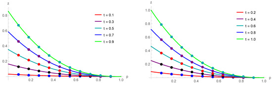
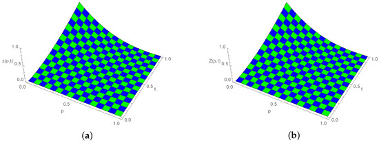
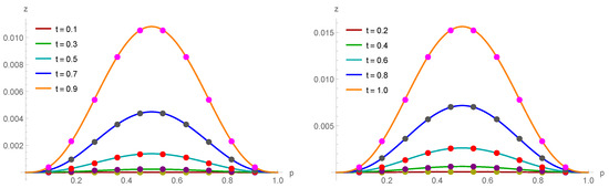
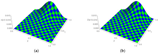
The proposed approach (12) was used to attain the numerical solution of the problem mentioned above. Figure 1 provides a comparison of the exact and approximate solutions at various time points with $h=\frac{1}{80}$, $\Delta t=\frac{1}{100}$ and $\alpha =1.5$. Figure 2 shows a three-dimensional (3D) comparison of the approximate (right) and exact (left) solutions. For various $\alpha$ values with a range of $1\le \alpha \le 2$, the absolute errors are determined and compared with the results presented in [21] in Table 1, Table 2 and Table 3. For $\alpha =1.6$, the absolute errors are determined and compared with the results presented in [38] in Table 4. In Table 5, for different values of $\alpha$, the approximate solutions are listed.

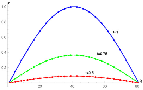
Figure 1. The numerical (circles) and exact (solid lines) solutions for various points in time when $h=\frac{1}{80},\Delta t=\frac{1}{100},t=1\mathrm{and}\alpha =1.5$ for Example 1.

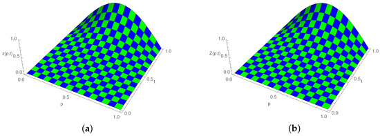
Figure 2. Three-dimensional plot for exact and approximate solutions, when $h=\frac{1}{80}$, $\Delta t=\frac{1}{100}$, $t=1$ and $\alpha =1.5$ for Example 1. (a) Exact solution; (b) Numerical solution.

Table 1. Absolute errors with $\alpha =1.5$ for Example 1.

	CTBS [21]	Presented Method
	CPU Time(s) 3484.98	CPU Time(s) 353.6875
p	$h=\frac{1}{80},\Delta t=0.001$	$h=\frac{1}{80},\Delta t=0.001$
$0.1$	$2.2437\times {10}^{-4}$	$3.7667\times {10}^{-5}$
$0.2$	$4.4180\times {10}^{-4}$	$7.0999\times {10}^{-5}$
$0.3$	$6.3346\times {10}^{-4}$	$9.6627\times {10}^{-5}$
$0.4$	$7.6861\times {10}^{-4}$	$1.1255\times {10}^{-4}$
$0.5$	$8.1773\times {10}^{-4}$	$1.1793\times {10}^{-4}$
$0.6$	$7.6861\times {10}^{-4}$	$1.1255\times {10}^{-4}$
$0.7$	$6.3346\times {10}^{-4}$	$9.6627\times {10}^{-5}$
$0.8$	$4.4180\times {10}^{-4}$	$7.0999\times {10}^{-5}$
$0.9$	$2.2437\times {10}^{-4}$	$3.7667\times {10}^{-5}$

Table 2. Absolute errors with $\alpha =1.7$ for Example 1.

	CTBS [21]	Presented Method
	CPU Time(s) 3503.70	CPU Time(s) 358.2656
p	$h=\frac{1}{80},\Delta t=0.001$	$h=\frac{1}{80},\Delta t=0.001$
$0.1$	$2.8566\times {10}^{-4}$	$1.2052\times {10}^{-5}$
$0.2$	$5.5578\times {10}^{-4}$	$2.2820\times {10}^{-5}$
$0.3$	$7.8594\times {10}^{-4}$	$3.1232\times {10}^{-5}$
$0.4$	$9.4376\times {10}^{-4}$	$3.6548\times {10}^{-5}$
$0.5$	$1.0003\times {10}^{-3}$	$3.8361\times {10}^{-5}$
$0.6$	$9.4376\times {10}^{-4}$	$3.6548\times {10}^{-5}$
$0.7$	$7.8594\times {10}^{-4}$	$3.1232\times {10}^{-5}$
$0.8$	$5.5578\times {10}^{-4}$	$2.2820\times {10}^{-5}$
$0.9$	$2.8566\times {10}^{-4}$	$1.2052\times {10}^{-5}$

Table 3. Absolute errors with $\alpha =1.9$ for Example 1.

	CTBS [21]	Presented Method
	CPU Time(s) 3489.45	CPU Time(s) 254.8750
p	$h=\frac{1}{80},\Delta t=0.001$	$h=\frac{1}{80},\Delta t=0.001$
$0.1$	$4.8172\times {10}^{-4}$	$1.7910\times {10}^{-5}$
$0.2$	$9.2384\times {10}^{-4}$	$3.3370\times {10}^{-5}$
$0.3$	$1.2844\times {10}^{-3}$	$4.4751\times {10}^{-5}$
$0.4$	$1.5211\times {10}^{-3}$	$5.1494\times {10}^{-5}$
$0.5$	$1.6051\times {10}^{-3}$	$5.3699\times {10}^{-5}$
$0.6$	$1.5211\times {10}^{-3}$	$5.1494\times {10}^{-5}$
$0.7$	$1.2844\times {10}^{-3}$	$4.4751\times {10}^{-5}$
$0.8$	$9.2384\times {10}^{-4}$	$3.3370\times {10}^{-5}$
$0.9$	$4.8172\times {10}^{-4}$	$1.7910\times {10}^{-5}$

Table 4. Comparison of absolute errors for Example 1 with $\alpha =1.6$, $\Delta t=0.001$ and $N=100$.

		RECBS [38]	Proposed Method
$\mathit{t}$	$\mathit{p}$
	$0.4$	$1.1769\times {10}^{-7}$	$2.0024\times {10}^{-8}$
0.4	$0.6$	$1.0126\times {10}^{-6}$	$5.3950\times {10}^{-7}$
	$0.8$	$7.2740\times {10}^{-6}$	$3.3133\times {10}^{-7}$

Table 5. Approximate solution for several $\alpha$ values, where $h=\frac{1}{40},t=1,\Delta t=0.01,\nu =-0.0000009$ for Example 1.

p	$\mathit{\alpha }=1.6$	$\mathit{\alpha }=1.8$	$\mathit{\alpha }=1.9$	$\mathit{\alpha }=1.95$	$\mathit{\alpha }=1.99$	$\mathit{\alpha }=1.999$
$0.1$	$0.309102$	$0.309832$	$0.310767$	$0.311496$	$0.312251$	$0.312446$
$0.2$	$0.587949$	$0.589326$	$0.591093$	$0.592473$	$0.593903$	$0.594272$
$0.3$	$0.809245$	$0.811122$	$0.813536$	$0.815423$	$0.817381$	$0.817886$
$0.4$	$0.951327$	$0.953516$	$0.956337$	$0.958543$	$0.960835$	$0.961426$
$0.5$	$1.000290$	$1.002580$	$1.007850$	$1.007850$	$1.010260$	$1.010880$
$0.6$	$0.951327$	$0.953516$	$0.956337$	$0.958543$	$0.960835$	$0.961426$
$0.7$	$0.809245$	$0.811122$	$0.813536$	$0.815423$	$0.817381$	$0.817886$
$0.8$	$0.587949$	$0.589326$	$0.591093$	$0.592473$	$0.593903$	$0.594272$
$0.9$	$0.309102$	$0.309832$	$0.310767$	$0.311496$	$0.3122514$	$0.312446$

Example 2

([46]). Consider the linear inhomogeneous TFKGE (1) when ${\delta }_1=1,{\delta }_2=0,0\le p\le 1,t>0,{\varphi }_0(p)={\varphi }_1(p)=0,{\psi }_0(t)=0$ and

$$\begin{array}{c}\hfill {\psi }_1(t)\approx 6\frac{t^{\alpha +1}}{\Gamma (\alpha +2)}-30\frac{t^{\alpha +3}}{\Gamma (\alpha +4)}+(\alpha +1)\left(6\frac{t^{\alpha +1}}{\Gamma (\alpha +2)}-30\frac{t^{\alpha +3}}{\Gamma (\alpha +4)}\right)+{(\alpha -1)}^2\left(30\frac{t^{2\alpha +1}}{\Gamma (2\alpha +2)}+66\frac{t^{2\alpha +3}}{\Gamma (2\alpha +4)}\right).\end{array}$$

The force term is

$$q(p,t)=6p^{3}t+(p^3-6p)t^3.$$

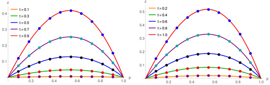
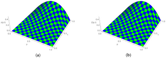
The exact solution of the problem is $z(p,t)=p^3{t}^3$. Using the scheme (12), the approximate solutions are attained for a variety of $\alpha$ values, and the results are shown in Table 6. The approximate solutions for various $\alpha$ values of Example 2 are displayed in Figure 3. Figure 4 provides a three-dimensional (3D) comparison of exact (left) and approximate (right) solutions.

Table 6. Approximate solutions for several $\alpha$ values where $h=\frac{1}{40}$, $t=1$, $\Delta t=0.01$ and $\nu =-0.0007$ for Example 2.

p	$\mathit{\alpha }=1.6$	$\mathit{\alpha }=1.8$	$\mathit{\alpha }=1.9$	$\mathit{\alpha }=1.95$	$\mathit{\alpha }=1.99$	$\mathit{\alpha }=1.999$
$0.1$	$0.003111$	$0.002671$	$0.004456$	$0.003045$	$0.001653$	$0.001315$
$0.2$	$0.011775$	$0.010599$	$0.014395$	$0.011648$	$0.009028$	$0.008397$
$0.3$	$0.031589$	$0.029174$	$0.035478$	$0.031602$	$0.028040$	$0.027188$
$0.4$	$0.068255$	$0.064053$	$0.073604$	$0.068899$	$0.064699$	$0.063703$
$0.5$	$0.127654$	$0.121295$	$0.134813$	$0.129604$	$0.125065$	$0.123999$
$0.6$	$0.215937$	$0.207469$	$0.225172$	$0.219817$	$0.215252$	$0.214190$
$0.7$	$0.339672$	$0.329778$	$0.350752$	$0.345687$	$0.341452$	$0.340477$
$0.8$	$0.506032$	$0.496257$	$0.517642$	$0.513432$	$0.509970$	$0.509181$
$0.9$	$0.723055$	$0.716078$	$0.731981$	$0.729376$	$0.727265$	$0.726788$

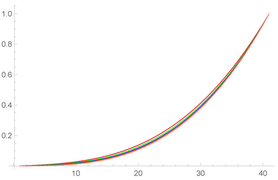
Figure 3. Approximate solution for various $\alpha$ values when $h=\frac{1}{40}$, $\Delta t=\frac{1}{100}$ and $t=1$ for Example 2.

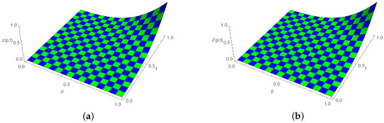
Figure 4. Three-dimensional plot for exact and approximate solutions, when $h=\frac{1}{40}$, $\Delta t=\frac{1}{100}$, $t=1$ and $\alpha =1.5$ for Example 2. (a) Exact solution; (b) Numerical solution.

Example 3

([38]). Consider the nonlinear TFKGE (1) with ${\delta }_1=0$, ${\delta }_2=1$, $0\le p\le 1$, ${\varphi }_0(p)={\varphi }_1(p)=0$, ${\psi }_0(t)=t^{\frac{3}{2}}$, ${\psi }_1(t)=0$, and the force term

$$q(p,t)=\frac{\Gamma \left(\frac{5}{2}\right)}{\Gamma \left(\frac{5}{2}-\alpha \right)}{(1-p)}^{\frac{5}{2}}{t}^{\frac{3}{2}-\alpha }-\frac{15}{4}{(1-p)}^{\frac{1}{2}}{t}^{\frac{3}{2}}+h(z(p,t)),$$

where $h(z(p,t))={(z(p,t))}^2$, and $z(p,t)={(1-p)}^{\frac{5}{2}}{t}^{\frac{3}{2}}$ is the exact solution of the given problem. Using Scheme (12), the approximate solutions were obtained, and the results are shown in Table 7. In Table 8, the comparison of error norms with [38] is listed. For $\alpha =1.6$, the absolute errors are determined and compared with the results presented in [38] in Table 9. Figure 5 provides a comparison of the exact and approximate solutions at various time points with $h=\frac{1}{25}$, $\Delta t=\frac{1}{200}$ and $\alpha =1.5$. Figure 6 shows a three-dimensional (3D) comparison of the approximate (right) and exact (left) solutions.

Table 7. Absolute errors at $t=1$, $\alpha =1.5$, $N=20$ and $\Delta t=0.01$ for Example 3.

p	Exact Solution	Approximate Solution	Absolute Errors
0.1	$0.768433$	$0.768433$	$1.1797\times {10}^{-9}$
0.2	$0.572433$	$0.572318$	$1.1557\times {10}^{-4}$
0.3	$0.409963$	$0.409708$	$2.5557\times {10}^{-4}$
0.4	$0.278855$	$0.278489$	$3.6557\times {10}^{-4}$
0.5	$0.176777$	$0.176360$	$4.1671\times {10}^{-4}$
0.6	$0.101193$	$0.100795$	$3.9818\times {10}^{-4}$
0.7	$0.049295$	$0.048983$	$3.1229\times {10}^{-4}$
0.8	$0.017889$	$0.017716$	$1.7206\times {10}^{-4}$
0.9	$0.003162$	$0.003158$	$3.9026\times {10}^{-6}$

Table 8. Comparison of error norms for Example 3 with $\alpha =1.3$ and $\Delta t=0.001$.

	RECBS [38]		Proposed Method
$\mathit{N}$	${\mathit{L}}_{\infty }$	${\mathit{L}}_{\mathbf{2}}$	${\mathit{L}}_{\infty }$	${\mathit{L}}_{\mathbf{2}}$
10	$3.1950\times {10}^{-2}$	$2.9355\times {10}^{-2}$	$1.7841\times {10}^{-3}$	$1.39087\times {10}^{-3}$
20	$9.0451\times {10}^{-3}$	$8.7109\times {10}^{-3}$	$1.7788\times {10}^{-4}$	$1.0508\times {10}^{-4}$
40	$2.4778\times {10}^{-3}$	$2.2128\times {10}^{-3}$	$3.3796\times {10}^{-5}$	$2.1677\times {10}^{-5}$
80	$6.3842\times {10}^{-4}$	$5.9376\times {10}^{-4}$	$1.5214\times {10}^{-5}$	$8.4009\times {10}^{-6}$

Table 9. Comparison of absolute errors for Example 3 with $\alpha =1.6$, $\Delta t=0.001$ and $N=100$.

		RECBS [38]	Proposed Method
$\mathit{t}$	$\mathit{p}$
	$0.4$	$1.6174\times {10}^{-5}$	$6.7324\times {10}^{-6}$
0.4	$0.6$	$6.3939\times {10}^{-6}$	$3.2045\times {10}^{-6}$
	$0.8$	$5.1612\times {10}^{-6}$	$4.4024\times {10}^{-7}$
	$0.4$	$2.4030\times {10}^{-5}$	$1.7690\times {10}^{-6}$
$0.8$	$0.6$	$6.7766\times {10}^{-6}$	$6.7009\times {10}^{-7}$
	$0.8$	$3.5003\times {10}^{-6}$	$8.4648\times {10}^{-8}$

Figure 5. Exact results (circles) and approximate solutions (solid lines) at various temporal stages for Example 3.

Figure 6. Three-dimensional plot for exact and approximate solutions, when $h=\frac{1}{16}$, $\Delta t=\frac{1}{1000}$, $t=1$ and $\alpha =1.5$ for Example 3. (a) Exact solution; (b) Numerical solution.

Example 4

([19,39]). Consider the linear TFKGE (1) with ${\delta }_1=1$, ${\delta }_2=0$, $0\le p\le 1$, ${\varphi }_0(p)={\varphi }_1(p)=0$, ${\psi }_0(t)={\psi }_1(t)=0$, and the force term

$$q(p,t)=\frac{2t^{2-\alpha }}{(2-\alpha )\Gamma (2-\alpha )}(e-e^p)sin(p)+t^2(2e-e^p)sin(p)+2t^2{e}^{p}cos(p),$$

where $z(p,t)=t^2(e-e^p)sin(p)$ is the exact solution of the given problem. The approximate solutions are demonstrated in Table 10. In Table 11, the comparison of error norms with [19,39] is expressed. Table 12 displays the analysis of error norms in the spatial direction. Figure 7 expounds the comparison of the exact and approximate solutions at various time stages with $h=\frac{1}{45}$, $\Delta t=\frac{1}{400}$ and $\alpha =1.5$. Figure 8 shows a three-dimensional (3D) comparison of the approximate (right) and exact (left) solutions.

Table 10. Absolute errors at $t=1$, $\alpha =1.6$, $N=50$ and $\Delta t=0.01$ for Example 4.

p	Exact Solution	Approximate Solution	Absolute Errors
0.1	$0.161042$	$0.161075$	$3.3088\times {10}^{-5}$
0.2	$0.297384$	$0.297481$	$9.7460\times {10}^{-5}$
0.3	$0.404397$	$0.404553$	$1.5594\times {10}^{-4}$
0.4	$0.477605$	$0.477788$	$1.8283\times {10}^{-4}$
0.5	$0.512775$	$0.512940$	$1.6518\times {10}^{-4}$
0.6	$0.506012$	$0.506116$	$1.0407\times {10}^{-4}$
0.7	$0.453870$	$0.453886$	$1.5793\times {10}^{-5}$
0.8	$0.353471$	$0.353404$	$6.7097\times {10}^{-5}$
0.9	$0.202630$	$0.202535$	$9.4895\times {10}^{-5}$

Table 11. Comparison of error norm for Example 4 with $\alpha =1.75$ and $h=\frac{1}{20}$.

	Fourth-Order CFD [19]	Sixth-Order CFD [39]	Proposed Method
$\mathbf{\Delta }\mathit{t}$	${\mathit{L}}_{\infty }$	${\mathit{L}}_{\infty }$	${\mathit{L}}_{\infty }$	${\mathit{L}}_{\mathbf{2}}$
$\frac{1}{10}$	$3.7014\times {10}^{-3}$	$3.7014\times {10}^{-3}$	$1.2528\times {10}^{-3}$	$8.0189\times {10}^{-4}$
$\frac{1}{20}$	$1.5270\times {10}^{-3}$	$1.5270\times {10}^{-3}$	$7.4684\times {10}^{-4}$	$4.7374\times {10}^{-4}$
$\frac{1}{40}$	$6.2904\times {10}^{-4}$	$6.2903\times {10}^{-4}$	$4.0106\times {10}^{-4}$	$2.3141\times {10}^{-4}$
$\frac{1}{80}$	$2.5916\times {10}^{-4}$	$2.5916\times {10}^{-4}$	$1.9319\times {10}^{-4}$	$1.3117\times {10}^{-4}$
$\frac{1}{160}$	$1.0715\times {10}^{-4}$	$1.0714\times {10}^{-4}$	$1.0350\times {10}^{-4}$	$7.0761\times {10}^{-5}$

Table 12. Error norms for Example 4 with $\alpha =1.3$ and $\Delta t=0.01$.

N	${\mathit{L}}_{\mathit{\infty }}$	${\mathit{L}}_2$
10	$4.7454\times {10}^{-4}$	$3.1201\times {10}^{-4}$
20	$3.9127\times {10}^{-4}$	$2.5294\times {10}^{-4}$
40	$2.7539\times {10}^{-4}$	$1.7101\times {10}^{-4}$
80	$1.1576\times {10}^{-4}$	$7.4440\times {10}^{-5}$

Figure 7. Exact results (circles) and approximate solutions (solid lines) at various temporal stages for Example 4.

Figure 8. Three-dimensional plot for exact and approximate solutions, when $h=\frac{1}{100}$, $\Delta t=\frac{1}{1000}$, $t=1$ and $\alpha =1.5$ for Example 4. (a) Exact solution; (b) Numerical solution.

Example 5

([40]). Consider the nonlinear TFKGE (1) with ${\delta }_1=0$, ${\delta }_2=2.5exp(p)$, $0\le p\le 1$, ${\varphi }_0(p)={\varphi }_1(p)=0$, ${\psi }_0(t)={\psi }_1(t)=0$, and the force term

$$q(p,t)=\frac{\Gamma (3+\alpha )}{2}{p}^3{(1-p)}^3{t}^2+(30p^4-60p^3+36p^2-6p)t^{2+\alpha }+2.5exp(p)h(z(p,t)),$$

where $h(z(p,t))={(z(p,t))}^{\frac{3}{2}}$, and $z(p,t)=p^3{(1-p)}^3{t}^{2+\alpha }$ is the exact solution of the given problem. The approximate solutions are expressed in Table 13. In Table 14 and Table 15, the comparison of error norms with [40] is demonstrated. Figure 9 represents the comparison of the exact and approximate solutions at various time stages with $h=\frac{1}{100}$, $\Delta t=\frac{1}{500}$ and $\alpha =1.5$. Figure 10 expounds a three-dimensional (3D) comparison of the approximate (right) and exact (left) solutions.

Table 13. Absolute errors at $t=1$, $\alpha =1.7$, $N=50$ and $\Delta t=0.005$ for Example 5.

p	Exact Solution	Approximate Solution	Absolute Errors
0.1	$0.000729$	$0.000765$	$3.5848\times {10}^{-5}$
0.2	$0.004096$	$0.004140$	$4.4264\times {10}^{-5}$
0.3	$0.009261$	$0.009296$	$3.5240\times {10}^{-5}$
0.4	$0.013824$	$0.013847$	$2.2700\times {10}^{-5}$
0.5	$0.015625$	$0.015642$	$1.7253\times {10}^{-5}$
0.6	$0.013824$	$0.013847$	$2.2741\times {10}^{-5}$
0.7	$0.009261$	$0.009296$	$3.5287\times {10}^{-5}$
0.8	$0.004096$	$0.004140$	$4.4293\times {10}^{-5}$
0.9	$0.000729$	$0.000765$	$3.5860\times {10}^{-5}$

Table 14. Comparison of error norms for Example 5 with $\alpha =1.5$, $t=1$ and $\Delta t=0.01$.

	CBS FEM [40]		Proposed Method
$\mathit{h}$	${\mathit{L}}_{\infty }$	${\mathit{L}}_{\mathbf{2}}$	${\mathit{L}}_{\infty }$	${\mathit{L}}_{\mathbf{2}}$
$\frac{1}{4}$	$1.2132\times {10}^{-3}$	$9.3311\times {10}^{-4}$	$1.0187\times {10}^{-3}$	$8.8201\times {10}^{-4}$
$\frac{1}{8}$	$4.0649\times {10}^{-4}$	$2.8192\times {10}^{-4}$	$4.3799\times {10}^{-4}$	$3.0777\times {10}^{-4}$
$\frac{1}{10}$	$2.8491\times {10}^{-4}$	$1.8780\times {10}^{-4}$	$2.7494\times {10}^{-4}$	$1.7921\times {10}^{-4}$
$\frac{1}{20}$	$1.1357\times {10}^{-4}$	$6.3206\times {10}^{-5}$	$9.0879\times {10}^{-5}$	$6.0401\times {10}^{-5}$
$\frac{1}{40}$	$6.6852\times {10}^{-5}$	$3.8371\times {10}^{-5}$	$5.7708\times {10}^{-5}$	$3.6271\times {10}^{-5}$
$\frac{1}{80}$	$5.5051\times {10}^{-5}$	$3.4415\times {10}^{-5}$	$4.7187\times {10}^{-5}$	$2.9298\times {10}^{-5}$
$\frac{1}{100}$	$4.6700\times {10}^{-6}$	$2.5900\times {10}^{-6}$	$3.5269\times {10}^{-6}$	$2.2255\times {10}^{-6}$

Table 15. Comparison of error norms for Example 5 with $\alpha =1.3$, $t=1$ and $\Delta t=0.005$.

	CBS FEM [40]		Proposed Method
$\mathit{h}$	${\mathit{L}}_{\infty }$	${\mathit{L}}_{\mathbf{2}}$	${\mathit{L}}_{\infty }$	${\mathit{L}}_{\mathbf{2}}$
$\frac{1}{4}$	$1.1779\times {10}^{-3}$	$9.1627\times {10}^{-4}$	$1.0512\times {10}^{-3}$	$8.9937\times {10}^{-4}$
$\frac{1}{8}$	$4.1643\times {10}^{-4}$	$2.7159\times {10}^{-4}$	$4.0370\times {10}^{-4}$	$1.9420\times {10}^{-4}$
$\frac{1}{10}$	$2.5651\times {10}^{-4}$	$1.7561\times {10}^{-4}$	$2.3485\times {10}^{-4}$	$1.4865\times {10}^{-4}$
$\frac{1}{20}$	$6.2482\times {10}^{-5}$	$4.4332\times {10}^{-5}$	$5.3501\times {10}^{-5}$	$3.7964\times {10}^{-5}$
$\frac{1}{40}$	$1.5783\times {10}^{-5}$	$1.1106\times {10}^{-5}$	$1.5305\times {10}^{-5}$	$1.0374\times {10}^{-5}$
$\frac{1}{80}$	$4.0630\times {10}^{-6}$	$2.7840\times {10}^{-6}$	$1.8171\times {10}^{-6}$	$1.1495\times {10}^{-6}$
$\frac{1}{100}$	$2.6600\times {10}^{-6}$	$1.7880\times {10}^{-6}$	$1.2686\times {10}^{-6}$	$8.3680\times {10}^{-7}$

Figure 9. Exact results (circles) and approximate solutions (solid lines) at various temporal stages for Example 5.

Figure 10. Three-dimensional plot for exact and approximate solutions, when $h=\frac{1}{60}$, $\Delta t=\frac{1}{500}$, $t=1$ and $\alpha =1.3$ for Example 5. (a) Exact solution; (b) Numerical solution.

7. Concluding Remarks

In this paper, we provide an ECBS-based numerical technique for the generalized nonlinear TFKGE. The standard finite difference techniques are used in this algorithm to estimate the CTFD, and the ECBS functions are employed to approximate the derivative in space. The convergence and stability of the scheme are also included in our research. The numerical scheme’s accuracy is demonstrated by contrasting the attained results with those provided in [19,21,38,39,40]. Comparing our technique numerically and graphically shows that it is more appropriate and computationally very effective. Therefore, with some modifications, our technique can be utilized to solve other classes of nonlinear FPDEs.

References

- Yousif, M.A.; Mahmood, B.A. Approximate solutions for solving the Klein-Gordon and sine-Gordon equations. J. Assoc. Arab. Univ. Basic Appl. Sci. 2017, 22, 83–90. [Google Scholar] [CrossRef]
- Yusufoğlu, E. The variational iteration method for studying the Klein-Gordon equation. Appl. Math. Lett. 2008, 21, 669–674. [Google Scholar] [CrossRef]
- Odibat, Z.; Momani, S. The variational iteration method: An efficient scheme for handling fractional partial differential equations in fluid mechanics. Comput. Math. Appl. 2009, 58, 2199–2208. [Google Scholar] [CrossRef]
- Golmankhaneh, A.K.; Baleanu, D. On nonlinear fractional Klein-Gordon equation. Signal Process. 2011, 91, 446–451. [Google Scholar] [CrossRef]
- Batiha, B.; Noorani, M.S.M.; Hashim, I. Numerical solution of sine-Gordon equation by variational iteration method. Phys. Lett. A 2007, 370, 437–440. [Google Scholar] [CrossRef]
- Kurulay, M. Solving the fractional nonlinear Klein-Gordon equation by means of the homotopy analysis method. Adv. Differ. Equ. 2012, 2012, 187. [Google Scholar] [CrossRef]
- Hariharan, G. Wavelet method for a class of fractional Klein-Gordon equations. J. Comput. Nonlinear Dyn. 2013, 8, 021008. [Google Scholar] [CrossRef]
- Hepson, O.E.; Korkmaz, A.; Dag, I. On the numerical solution of Klein-Gordon equation by exponential B-spline collocation method. Commun. Fac. Sci. Univ.-Ank.-Ser. Math. Stat. 2019, 68, 412–421. [Google Scholar] [CrossRef]
- Dehghan, M.; Abbaszadeh, M.; Mohebbi, A. An implicit RBF meshless approach for solving the time fractional nonlinear sine-Gordon and Klein-Gordon equations. Eng. Anal. Bound. Elem. 2015, 50, 412–434. [Google Scholar] [CrossRef]
- Zhang, Y. Time-fractional Klein-Gordon equation: Formulation and solution using variational methods. WSEAS Trans. Math. 2016, 15, 206–214. [Google Scholar]
- Chen, H.; Lü, S.; Chen, W. A fully discrete spectral method for the non-linear time fractional Klein-Gordon equation. Taiwan. J. Math. 2017, 21, 231–251. [Google Scholar] [CrossRef]
- Nagy, A.M. Numerical solution of time fractional nonlinear Klein-Gordon equation using Sinc-Chebyshev collocation method. Appl. Math. Comput. 2017, 310, 139–148. [Google Scholar] [CrossRef]
- El-Sayed, S.M. The decomposition method for studying the Klein-Gordon equation. Chaos Solitons Fractals 2003, 18, 1025–1030. [Google Scholar] [CrossRef]
- Kaya, D.; El-Sayed, S.M. A numerical solution of the Klein-Gordon equation and convergence of the decomposition method. Appl. Math. Comput. 2004, 156, 341–353. [Google Scholar] [CrossRef]
- Cui, M. Fourth-order compact scheme for the one-dimensional sine-Gordon equation. Numer. Methods Partial. Differ. Equ. Int. J. 2009, 25, 685–711. [Google Scholar] [CrossRef]
- Jafari, H.; Saeidy, M.; Firoozjaee, M.A. Solving nonlinear Klein-Gordon equation with a quadratic nonlinear term using homotopy analysis method. Iran. J. Optim. 2010, 2, 130–138. [Google Scholar]
- Vong, S.; Wang, Z. A compact difference scheme for a two dimensional fractional Klein-Gordon equation with Neumann boundary conditions. J. Comput. Phys. 2014, 274, 268–282. [Google Scholar] [CrossRef]
- Jafari, H.; Tajadodi, H.; Kadkhoda, N.; Baleanu, D. Fractional subequation method for Cahn-Hilliard and Klein-Gordon equations. Abstr. Appl. Anal. 2013, 2013, 587179. [Google Scholar] [CrossRef]
- Mohebbi, A.; Abbaszadeh, M.; Dehghan, M. High-order difference scheme for the solution of linear time fractional Klein-Gordon equations. Numer. Methods Partial. Differ. Equ. 2014, 30, 1234–1253. [Google Scholar] [CrossRef]
- Vong, S.; Wang, Z. A high-order compact scheme for the nonlinear fractional Klein-Gordon equation. Numer. Methods Partial. Differ. Equ. 2015, 31, 706–722. [Google Scholar] [CrossRef]
- Yaseen, M.; Abbas, M.; Ahmad, B. Numerical simulation of the nonlinear generalized time-fractional Klein-Gordon equation using cubic trigonometric B-spline functions. Math. Methods Appl. Sci. 2021, 44, 901–916. [Google Scholar] [CrossRef]
- Kamran, M.; Majeed, A.; Li, J. On numerical simulations of time fractional Phi-four equation using Caputo derivative. Comput. Appl. Math. 2021, 40, 257. [Google Scholar] [CrossRef]
- Fang, J.; Nadeem, M.; Habib, M.; Karim, S.; Wahash, H.A. A new iterative method for the approximate solution of Klein-Gordon and sine-Gordon equations. J. Funct. Spaces 2022, 2022, 5365810. [Google Scholar] [CrossRef]
- Sweilam, N.H.; Khader, M.M.; Mahdy, A.M.S. On the numerical solution for the linear fractional Klein-Gordon equation using Legendre pseudospectral method. Int. J. Math. Comput. Appl. Res. 2012, 2, 1–10. [Google Scholar]
- Abuteen, E.; Freihat, A.; Al-Smadi, M.; Khalil, H.; Khan, R.A. Approximate series solution of nonlinear, fractional Klein-Gordon equations using fractional reduced differential transform method. J. Math. Stat. 2016, 12, 23–33. [Google Scholar] [CrossRef]
- Bülbül, B.; Sezer, M. A new approach to numerical solution of nonlinear Klein-Gordon equation. Math. Probl. Eng. 2013, 2013, 869749. [Google Scholar]
- Hesameddini, E.; Fotros, F. Solution for time-fractional coupled Klein-Gordon Schrödinger equation using decomposition method. Int. Math. Forum 2012, 7, 1047–1056. [Google Scholar]
- Abbasbandy, S. Numerical solution of non-linear Klein-Gordon equations by variational iteration method. Int. J. Numer. Methods Eng. 2007, 70, 876–881. [Google Scholar] [CrossRef]
- Singh, J.; Kumar, D.; Rathore, S. Application of homotopy perturbation transform method for solving linear and nonlinear Klein-Gordon equations. J. Inf. Comput. Sci. 2012, 7, 131–139. [Google Scholar]
- Schoenberg, I.J. Contributions to the problem of approximation of equidistant data by analytic functions. part B. on the problem of osculatory interpolation. a second class of analytic approximation formulae. Q. Appl. Math. 1946, 4, 112–141. [Google Scholar] [CrossRef]
- Shafiq, M.; Abdullah, F.A.; Abbas, M.; Alzaidi, A.S.M.; Riaz, M.B. Memory effect analysis using piecewise cubic B-spline of time fractional diffusion equation. Fractals 2022, 30, 2240270. [Google Scholar] [CrossRef]
- Shafiq, M.; Abbas, M.; El-Shewy, E.K.; Abdelrahman, M.A.E.; Abdo, N.F.; El-Rahman, A.A. Numerical investigation of the fractional diffusion wave equation with the Mittag–Leffler function. Fractal Fract. 2024, 8, 18. [Google Scholar] [CrossRef]
- Hepson, O.E. Generation of the trigonometric cubic B-spline collocation solutions for the Kuramoto-Sivashinsky (KS) equation. In AIP Conference Proceedings; AIP Publishing: Huntington, NY, USA, 2018; Volume 1978, pp. 1–5. [Google Scholar]
- Yadav, S.; Pandey, R.K.; Shukla, A.K. Numerical approximations of Atangana-Baleanu Caputo derivative and its application. Chaos Solitons Fractals 2019, 118, 58–64. [Google Scholar] [CrossRef]
- Majeed, A.; Kamran, M.; Iqbal, M.K.; Baleanu, D. Solving time fractional Burgers’ and Fisher’s equations using cubic B-spline approximation method. Adv. Differ. Equ. 2020, 2020, 175. [Google Scholar] [CrossRef]
- Mittal, R.C.; Jain, R. Numerical solutions of nonlinear Burgers’ equation with modified cubic B-splines collocation method. Appl. Math. Comput. 2012, 218, 7839–7855. [Google Scholar] [CrossRef]
- Tamsir, M.; Srivastava, V.K.; Jiwari, R. An algorithm based on exponential modified cubic B-spline differential quadrature method for nonlinear Burgers’ equation. Appl. Math. Comput. 2016, 290, 111–124. [Google Scholar] [CrossRef]
- Amin, M.; Abbas, M.; Iqbal, M.K.; Baleanu, D. Numerical treatment of time-fractional Klein-Gordon equation using redefined extended cubic B-spline functions. Front. Phys. 2020, 8, 288. [Google Scholar] [CrossRef]
- Soori, Z.; Aminataei, A. High-order difference scheme for the solution of linear time fractional Klein-Gordon equation. In Proceedings of the 47th Annual Iranian Mathematics Conference, Kharazmi University, Karaj, Iran, 28–31 August 2016. [Google Scholar]
- Karaagac, B.; Yusuf, U.C.A.R.; Yagmurlu, N.M.; Alaattin, E.S.E.N. A new perspective on the numerical solution for fractional klein gordon equation. J. Polytech. 2019, 22, 443–451. [Google Scholar] [CrossRef]
- Podlubny, I. Fractional Differential Equations; Academic Press: San Diego, CA, USA, 1999. [Google Scholar]
- Khader, M.M.; Adel, M.H. Numerical solutions of fractional wave equations using an efficient class of FDM based on the Hermite formula. Adv. Differ. Equ. 2016, 2016, 34. [Google Scholar] [CrossRef]
- Umer, A.; Abbas, M.; Shafiq, M.; Abdullah, F.A.; De la Sen, M.; Abdeljawad, T. Numerical solutions of Atangana-Baleanu time-fractional advection diffusion equation via an extended cubic B-spline technique. Alex. Eng. J. 2023, 74, 285–300. [Google Scholar] [CrossRef]
- Shafiq, M.; Abbas, M.; Abdullah, F.A.; Majeed, A.; Abdeljawad, T.; Alqudah, M.A. Numerical solutions of time fractional Burgers’ equation involving Atangana-Baleanu derivative via cubic B-spline functions. Results Phys. 2022, 34, 105244. [Google Scholar] [CrossRef]
- Shafiq, M.; Abbas, M.; Abualnaja, K.M.; Huntul, M.J.; Majeed, A.; Nazir, T. An efficient technique based on cubic B-spline functions for solving time-fractional advection diffusion equation involving Atangana-Baleanu derivative. Eng. Comput. 2022, 38, 901–917. [Google Scholar] [CrossRef] [PubMed]
- Turut, V.; Güzel, N. On solving partial differential equations of fractional order by using variational iteration method and multivariate Padé approximations. Eur. J. Pure Appl. Math. 2013, 6, 147–171. [Google Scholar]
Disclaimer/Publisher’s Note: The statements, opinions and data contained in all publications are solely those of the individual author(s) and contributor(s) and not of MDPI and/or the editor(s). MDPI and/or the editor(s) disclaim responsibility for any injury to people or property resulting from any ideas, methods, instructions or products referred to in the content. |
© 2024 by the authors. Licensee MDPI, Basel, Switzerland. This article is an open access article distributed under the terms and conditions of the Creative Commons Attribution (CC BY) license (https://creativecommons.org/licenses/by/4.0/).