Computational Analysis of Hemodynamic Indices in Multivessel Coronary Artery Disease in the Presence of Myocardial Perfusion Dysfunction

Abstract

Coronary artery disease (CAD) is one of the main causes of death in the world. Functional indices such as fractional flow reserve (FFR), coronary flow reserve (CFR) and instantaneous wave-free ratio (iFR) are used to estimate the severity of CAD. Approximately 30–50% of patients have residual myocardial ischaemia even after formally successful percutaneous coronary intervention (PCI). Myocardial perfusion impairment is one of the main factors responsible for recurrence. We propose a novel 1D model of coronary hemodynamics that takes into account myocardial contraction, stenoses and impaired microcirculation. It uses non-invasively acquired data. The model is able to simulate FFR and iFR with a mean relative error of 3% and a standard mean deviation of 0.04. We find that healthy FFR and iFR values in the short and long term do not always correspond to healthy CFR values and recovery of coronary blood flow. We also show that PCI of stenosis also improves hemodynamic indices in adjacent stenosed vessels, with a more pronounced effect in the long term.

1. Introduction

Coronary artery disease (CAD) is the leading cause of death worldwide. It accounts for 10–14% of all deaths. Coronary computed tomography angiography (CCTA) is one of the main diagnostic tools for assessing the degree of CAD. Currently, catheter-based fractional flow reserve (FFR) is considered the reference value for assessing the functional severity of CAD. It is used to determine the need for percutaneous coronary intervention (PCI) [1]. During drug-induced coronary hyperemia, which causes vasodilation, FFR is the ratio of the pressure distal to stenosis to the pressure anterior to the stenosis (or aortic pressure). FFR is a measure of the possible average blood pressure recovery in epicardial coronary arteries if stenosis is removed. Coronary flow reserve (CFR) and instantaneous wave-free ratio (iFR) are also useful in assessing the severity of CAD. CFR is the ratio of coronary blood flow (CBF) during pharmacological (drug-induced) hyperemia to resting CBF [2]. CFR is a measure of the maximum possible recovery of blood flow in large coronary arteries after PCI. CFR values help to understand the functional significance of CAD. However, CFR measurements are usually unavailable since accurate estimation of blood flow is hard to achieve in clinical practice. iFR is similar to FFR, but the measurement is made over the so-called wave-free period in diastole. It is also a ratio of distal coronary pressure and aortic pressure averaged over the same period [3]. Incorrect estimation of the wave-free interval can cause some errors. iFR is measured under normal conditions in the absence of hyperemia and drug administration. FFR, CFR and iFR characterize the severity of stenosis in large coronary arteries with a diameter of more than 0.5 mm.

Although the advantages of PCI for the treatment of CAD have been well established, approximately 30–50% of patients have residual myocardial ischaemia even after formally successful PCI. This is due to an increased risk of late restenosis, repeat revascularisation and adverse cardiac events. Identifying cases with potential post-operative complications has become a major concern in clinical practice. To improve decision making, the use of post-interventional FFR and/or CFR has recently been proposed in the evaluation of CAD.

The other improvement is achieved by myocardial CT perfusion (CTP). It provides a comprehensive assessment of myocardial microcirculation impairment and ischaemia [4]. CTP is performed by imaging the left ventricular myocardium during the first pass of the contrast bolus after administration of iodinated contrast through a catheter. The iodinated contrast agent attenuates X-rays in proportion to the contrast density in the tissue. This allows direct visualization of myocardial perfusion defects as hypoattenuating or non-enhancing regions.

There are two main correlated causes of CAD: stenosis of large coronary arteries and dysfunctional myocardial microcirculation [5,6]. This relationship is not always clear [7]: stenosis with low FFR value may be a reason to recommend PCI to restore blood flow in myocardial region downstream. However, due to the presence of dysfunctional microcirculatory region downstream, myocardial perfusion may still be low. This may lead to restenosis and recurrent ischaemia several months after PCI. In this case, PCI may not be the optimal choice of treatment. Many clinical studies have examined perfusion indices [8,9] or combined FFR with myocardial perfusion [10,11]. In modern mathematical models of coronary circulation, CTP data are rarely used for CAD severity assessment [12,13,14]. Many works take into account FFR, CFR or iFR regardless of the state of the myocardial microvasculature [15,16,17,18].

Reduced-order models of coronary circulation provide a powerful tool for diagnostics. 1D [15,17], 0D [19] and combined 1D-0D [14] approaches allow for a fast computations with adequate precision. The choice between 1D and 0D models is usually made based on the degree of flow detail required. In this work, we need to calculate three different hemodynamic indices in multiple arteries at a time. We use a well-developed and tested 1D model of coronary blood flow [20]. In this model, blood is considered to be viscous and incompressible and arteries are represented as a graph (network) of elastic tubes. We simplify 0D elements in our model to reduce the amount of parameters. Zero-dimensional elements in our model are reduced to resistances on terminal ends. We compute TPR for user-defined regions of the left coronary artery. In our model, there is a decrease in terminal resistance as the transmural perfusion ratio (TPR) increases. The resulting model is used as a computational tool for the estimation of changes in coronary hemodynamics from pre- to post-PCI in 11 patients.

We calculate blood flow indices (FFR, CFR and iFR) before PCI, immediately after surgery and in the long term (several months after PCI). Non-invasively collected patient data are used to set the parameters of the model. Our results show that the use of TPR data enhances the quality of the simulations. We obtained an average relative error of 3% with a standard mean deviation of 0.04. We find that healthy FFR and iFR values in the short and long term do not always correspond to healthy CFR values and recovery of coronary blood flow in the long term. Our simulations show that PCI of stenosis also increases hemodynamic index values in adjacent stenosed vessels, with a more pronounced effect in the long term.

The paper is organized as follows. In Section 2, we describe the 1D hemodynamic model and its main equations. Section 3 presents details on medical image processing. In Section 4, we describe the patient data. This section also contains the results of the simulations. Section 5 is a discussion of obtained results.

2. Mathematical Model of Coronary Hemodynamics

2.1. The Model of Bood Flow in a Single Vessel

This section presents a one-dimensional (1D) model of transient viscous incompressible fluid flow through a network of elastic tubes. In the following sections, we use this model to numerically simulate coronary blood flow and hemodynamic indices (FFR, CFR and iFR). This model is described in more detail in [13,21,22]. Here, we present the main equations and parts of the model that are important for stenoses and perfusion simulations.

The flow in any elastic tube (vessel) is described by mass and momentum balance equations.

$$\frac{\partial \mathbf{V}}{\partial t}+\frac{\partial \mathbf{F}\left(\mathbf{V}\right)}{\partial x}=\mathbf{G}\left(\mathbf{V}\right),$$

(1)

$$\mathbf{V}=\left(\begin{array}{c}A\\ u\end{array}\right),\mathbf{F}\left(\mathbf{V}\right)=\left(\begin{array}{c}Au\\ {\displaystyle u^2/2+p\left(A\right){\rho }^{-1}}\end{array}\right),\mathbf{G}\left(\mathbf{V}\right)=\left(\begin{array}{c}0\\ -8\pi \mu u{A}^{-1}\end{array}\right),$$

where t is time, x is the coordinate along the vessel, $\rho$ is the blood density (constant, 1.06 g/cm³), $A\left(t,x\right)$ is the cross-section area, p is the blood pressure, $u\left(t,x\right)$ is the blood flow velocity averaged over the cross-section, $\mu$ is the dynamic viscosity of the blood (constant). The wall-state equation defines the relationship between pressure and cross-section:

$$p\left(A\right)={\rho }_w{c}^{2}F\left(A\right),$$

(2)

where ${\rho }_w$ is the density of arterial wall, c is the pulse wave velocity in the unstressed vessel, and $F\left(A\right)$ is a specific function [23]:

$$F\left(A\right)=\left\{\begin{array}{cc}exp\left(\kappa -1\right)-1,\hfill & \kappa >1\hfill \\ ln\kappa ,\hfill & \kappa ⩽1\hfill \end{array}\right.,\eta =A{A}_0^{-1},$$

(3)

where $A_0$ is the area of the vessel at rest.

2.2. Boundary Conditions at Vascular Connections

We apply mass conservation at the connecting points of the vessel and ensure that the total pressure remains constant.

$$\sum _{k_i=k_1,k_2,\dots ,k_M}{\epsilon }_{k_i}{A}_{k_i}\left(t,{\tilde{x}}_{k_i}\right)u_{k_i}\left(t,{\tilde{x}}_{k_i}\right)=0,$$

(4)

$$p_{k_i}+\frac{\rho u^2\left(t,{\tilde{x}}_{k_i}\right)}{2}=p_{k_{i+1}}+\frac{\rho u^2\left(t,{\tilde{x}}_{k_{i+1}}\right)}{2},k_i=k_1,k_2,\dots ,k_{M-1},$$

(5)

where $k_i$ is the index of the connecting vessel, $i=1,\dots ,M$ (M—total amount of vessels at the connecting point), ${\epsilon }_{k_i}=1,{\tilde{x}}_{k_i}=L_{k_i}$ for vessels that are proximal to the connecting point (usually a single vessel), ${\epsilon }_{k_i}=-1,{\tilde{x}}_{k_i}=0$ for distal vessels and $L_{k_i}$ is the length of $k_i$-th vessel. We rarely have more than three vessels connecting at a single point.

The boundary conditions at vascular connections include compatibility conditions of (1) along outgoing characteristics. Their discretization at every time step leads to a nonlinear set of equations for $u_{k_i}(t_{n+1},{\tilde{x}}_{k_i})$ and $A_{k_i}(t_{n+1},{\tilde{x}}_{k_i})$.

2.3. Inflow Boundary Conditions

At the aortic root, we set a blood flow as a pre-defined function of time $Q_H\left(t\right)$

$$u\left(t,0\right)A\left(t,0\right)=Q_H\left(t\right).$$

(6)

$Q_H\left(t\right)$ is a sinusoidal function during ventricular systole and is set to zero during diastole:

$$Q_H\left(t\right)=\left\{\begin{array}{c}{\displaystyle {\displaystyle \frac{\pi SV}{2\tau \left(T\right)}}sin\left({\displaystyle \frac{\pi t}{\tau }}\right),0⩽t⩽\tau ,}\hfill \\ 0,\tau <t⩽T,\hfill \end{array}\right.$$

(7)

where parameters $SV$, T and $\tau$ are set according to the patient data. $SV$ can be derived from echocardiography. T is the duration of a cardiac cycle and can be easily calculated from the patient’s heart rate. $SV$ is the stroke volume of the left ventricle, T is the period of the cardiac cycle, and $\tau$ is the duration of the systolic phase and can be measured on ECG.

The inflow boundary conditions include compatibility conditions of (1) along with outgoing characteristics. Their discretization at every time step gives us a set of nonlinear equations that can be solved with Newton’s method to find $u(t_{n+1},0)$ and $A(t_{n+1},0)$.

2.4. Outflow Boundary Conditions

We assume a Poiseuille pressure drop over the microcirculatory region to set the outflow boundary conditions.

$$p_k\left(t,L_k\right)-p_{veins}=R_k\left(t,\tau \right)A_k\left(t,L_k\right)u_k\left(t,L_k\right),$$

(8)

where $p_{veins}=8$ mmHg.

The outflow boundary conditions include compatibility conditions of (1) along with the outgoing characteristics. Their discretization at every time step once again gives us a set of nonlinear equations for $u(t_{n+1},L_k)$ and $A(t_{n+1},L_k)$.

Systolic compression of endocardial coronary arteries by the myocardium is an important characteristic of coronary blood flow. This effect is taken into account by the function $R_k=R_k(t,\tau )$. We assume that the shape of a function $R_k(t,\tau )$ is similar to cardiac output $Q_H(t,\tau )$ (7)

$$R_k\left(t,\tau \right)=\left\{\begin{array}{c}{\displaystyle R_k+\left(R_k^{sys}-R_k\right)sin\left({\displaystyle \frac{\pi t}{\tau }}\right),0⩽t⩽\tau ,}\hfill \\ R_k,\tau <t⩽T.\hfill \end{array}\right.$$

(9)

The highest value of the peripheral resistance during the systole phase is set to $R_k^{sys}=3R_k$, where $R_k$ is the default terminal resistance value. $R_k$ is the resistance during during diastolic phase. This modification stops the blood flow in coronary arteries during the systolic phase. To simulate drug-induced hyperemia we decrease $R_k$ : $R_k^{hyp}=0.3R_k$ [15,17].

The following algorithm is used to evaluate $R_k$ for terminal vessels. First, we assume that

$$R_{tot}={\displaystyle \frac{P_{mean}-p_{veins}}{Q_{CO}}},$$

(10)

where $R_{tot}$ is the total resistance between arteries and veins. $P_{mean}$ is the blood pressure in major arteries averaged over time.

Secondly, the effective resistance of the aorta $R_a$ and the total effective resistance of all coronary region $R_{CBF}$ are estimated. Our assumption is that coronary blood flow (CBF) constitutes 5% of total cardiac output (CO), so $\left(Q_{CBF}=\beta Q_{CO}\right)$ and $\beta =0.05$. We calculate $R_a$ and $R_{CBF}$ from:

$$R_a=\frac{P_{mean}-p_{veins}}{\left(1-\beta \right)·Q_{CO}},R_{CBF}=\frac{P_{mean}-p_{veins}}{\beta Q_{CO}}$$

(11)

Thus, we have $R_{CBF}\approx 19R_a$.

Thirdly, the terminal resistances, $R_k$, are evaluated for each terminal coronary artery. We split $R_{CBF}$ across terminal resistances $R_k$ according to Murray’s law: $R_k$ is proportional to the diameter of the artery to the power of 2.27 [15]. We do not split $R_{CBF}$ directly into resistances of terminal arteries. We start by splitting it across left and right coronary arteries, and then this procedure is performed iteratively for each arterial connection until terminal vessels are reached [21].

After we prescribe terminal resistance $R_k$ to each terminal artery, we calibrate $R_k$ to account for myocardial perfusion impairment using CTP data. Contrast-enhanced tomographic perfusion (CTP) images demonstrate the brightness of the injected iodinated contrast agent in the arterial blood stream. The brightness of the contrast agent is directly proportional to blood flow, and thus the oxygen is delivered to surrounding tissues. In accordance with the specifications of the CTP workstation, data pertaining to the 16 standard zones are automatically provided. Software embedded within the system calculates the average attenuation density ($AD$) of subendocardial, midwall, and subepicardial layers of myocardium in each zone.

The degree of impaired perfusion is assessed by calculating the transmural perfusion ratio ($TPR$):

$$TPR={\displaystyle \frac{A{D}_{end}}{A{D}_{ep}}},$$

(12)

where $A{D}_{end}$ is subendocardial (inner) $AD$ and $A{D}_{ep}$ is subepicardial (outer) $AD$. It should be noted that TPR does not have a direct physiological meaning. Empirical analysis has the potential to enhance diagnostic performance [24]. It has been suggested that possible values of $TPR$ in the human myocardium are within the range of 0.0 to 1.4. Furthermore, it is believed that normal perfusion can be indicated by $TPR$ values greater than 1.0. Moderate perfusion abnormalities are associated with $TPR$ values between 0.95 and 1.0. $TPR$ between 0.6 and 0.95 indicates severe perfusion abnormalities. It is rare to observe $TPR$ values below 0.6.

We assume that low $TPR$ values correspond to increased resistances of the myocardium regions. We multiply each of the terminal resistances $R_k$ by ${\beta }_{TPR}$

$${\beta }_{TPR}=\left\{\begin{array}{c}1,TPR⩾1.4\hfill \\ a+bexp\left(c·TPR\right),TPR<1.4\hfill \end{array}\right.$$

(13)

We set the empirical values of $a,b$ and c so that ${\beta }_{TPR}=1$ for $TP{R}_k=1.4$, ${\beta }_{TPR}=2$ for $TPR=0.6$ and ${\beta }_{TPR}=4$ for $TPR=0.2$ in accordance with clinical practice. Thus, we have

$$a=2+2/\sqrt{3},b=\sqrt{{\displaystyle \frac{{(4-a)}^3}{2-a}}},c=5ln{\displaystyle \frac{4-a}{b}}.$$

(14)

The hyperbolic system (1) is solved numerically for each vessel using the grid-characteristic method [25]. Newton’s method is employed to solve the system of nonlinear algebraic equations pertaining to the vessel’s junctions (4), (5), aortic root (6) and at the outflow borders of terminal vessels (8).

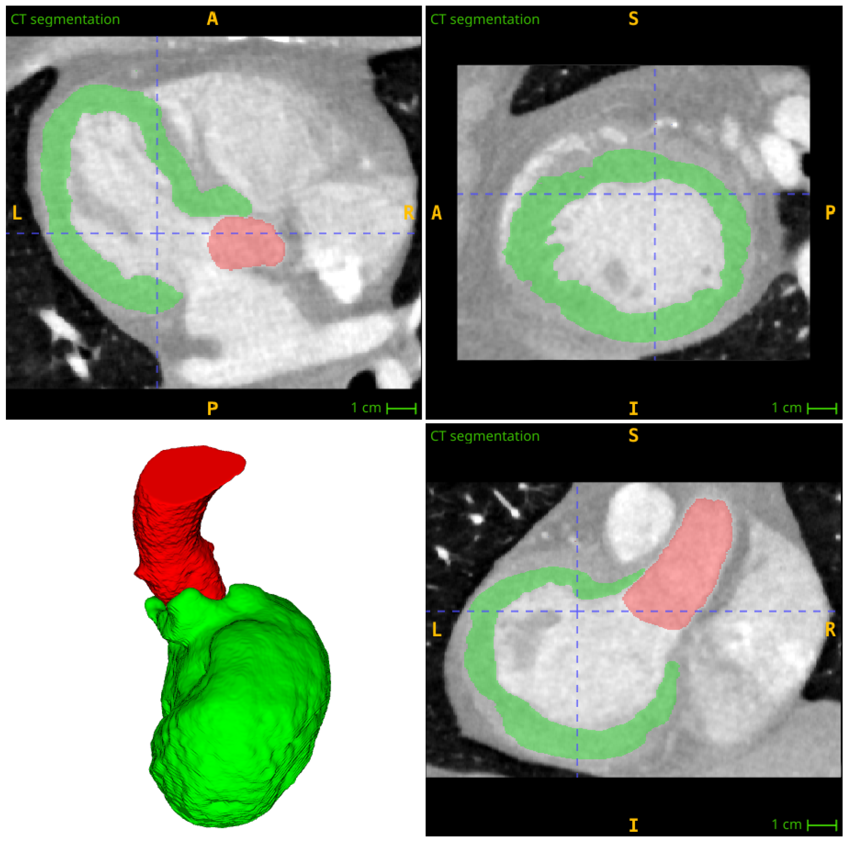
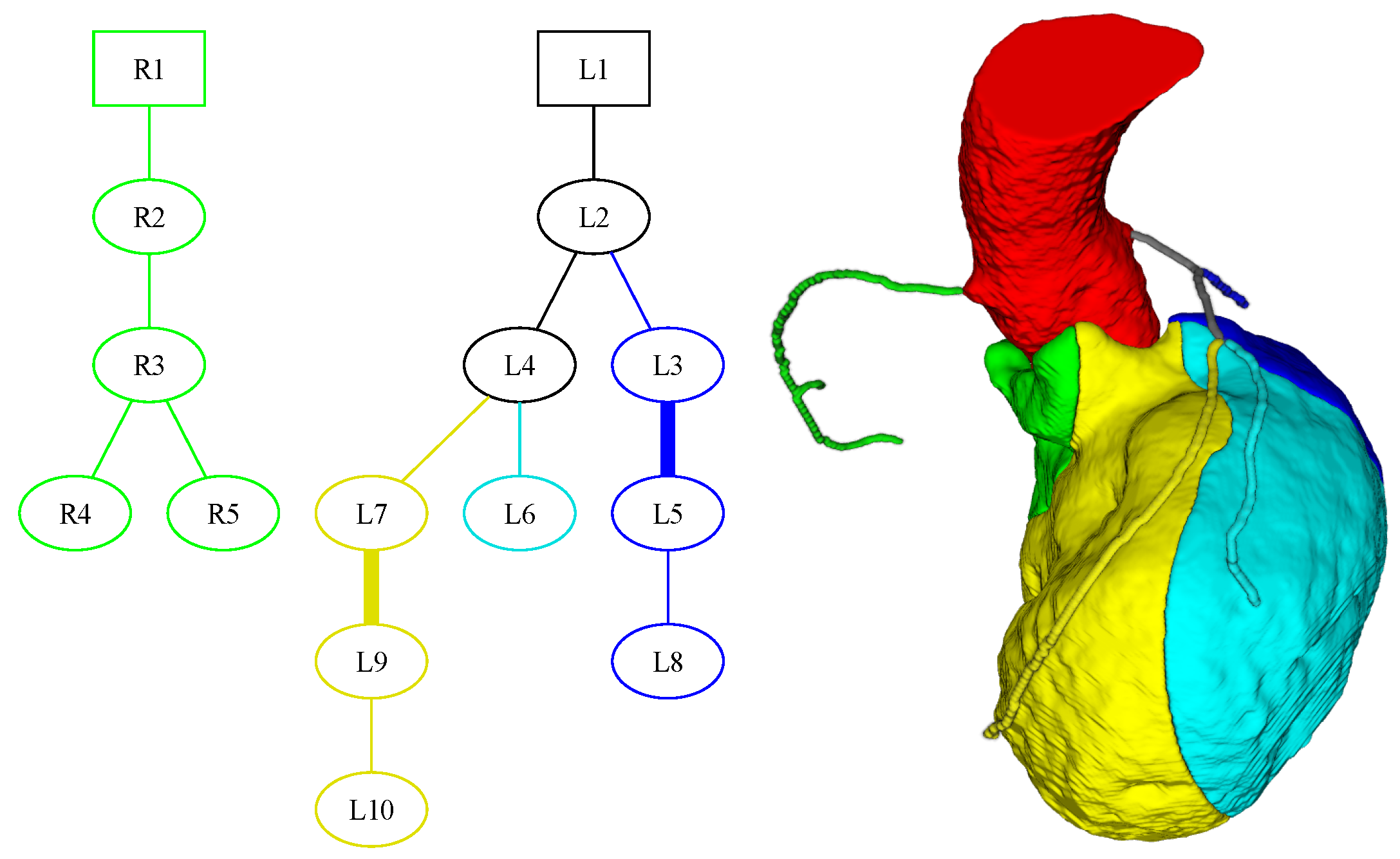
3. Segmentation and Partitioning of Coronary Vessels and Microcirculation

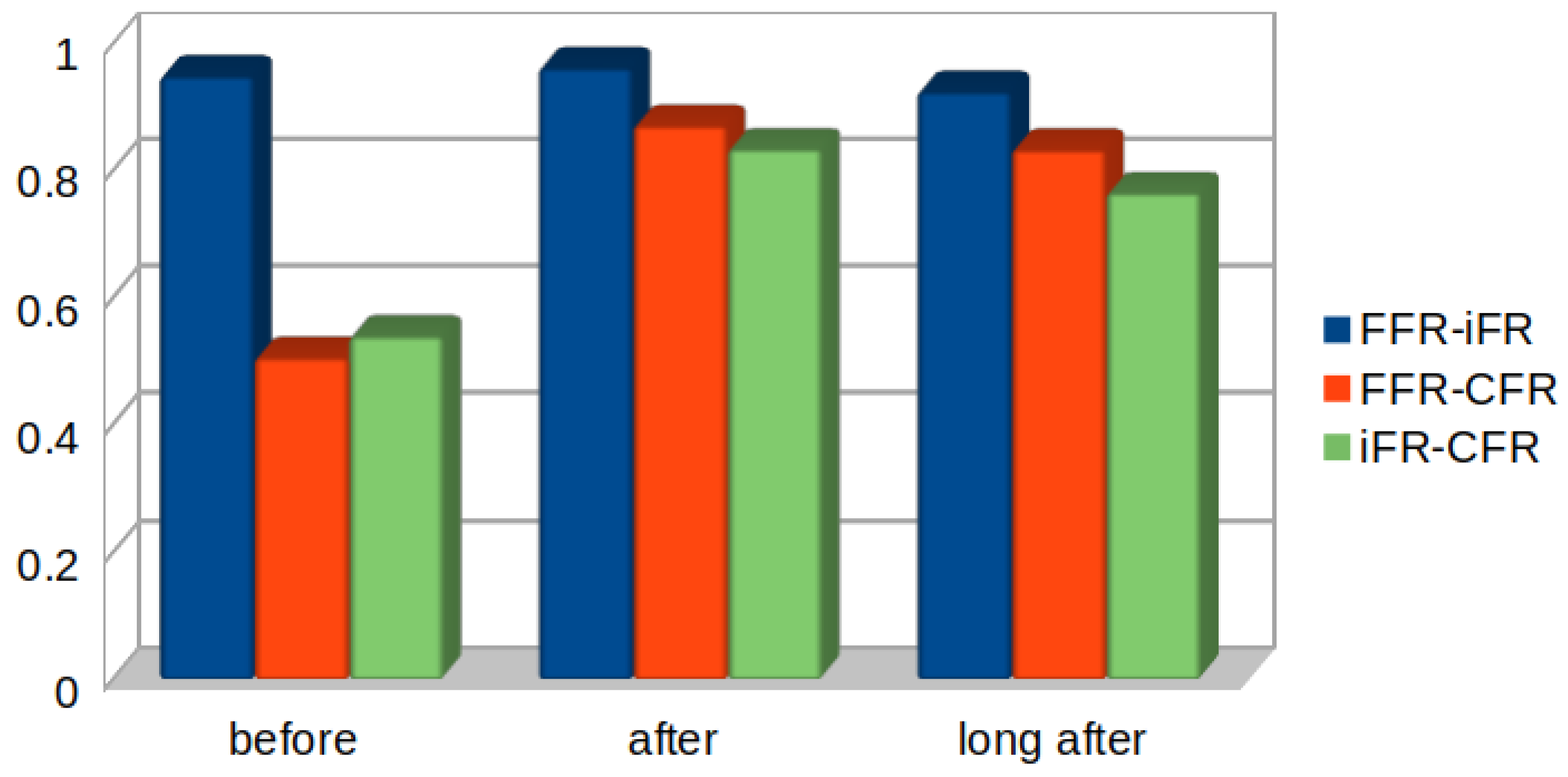
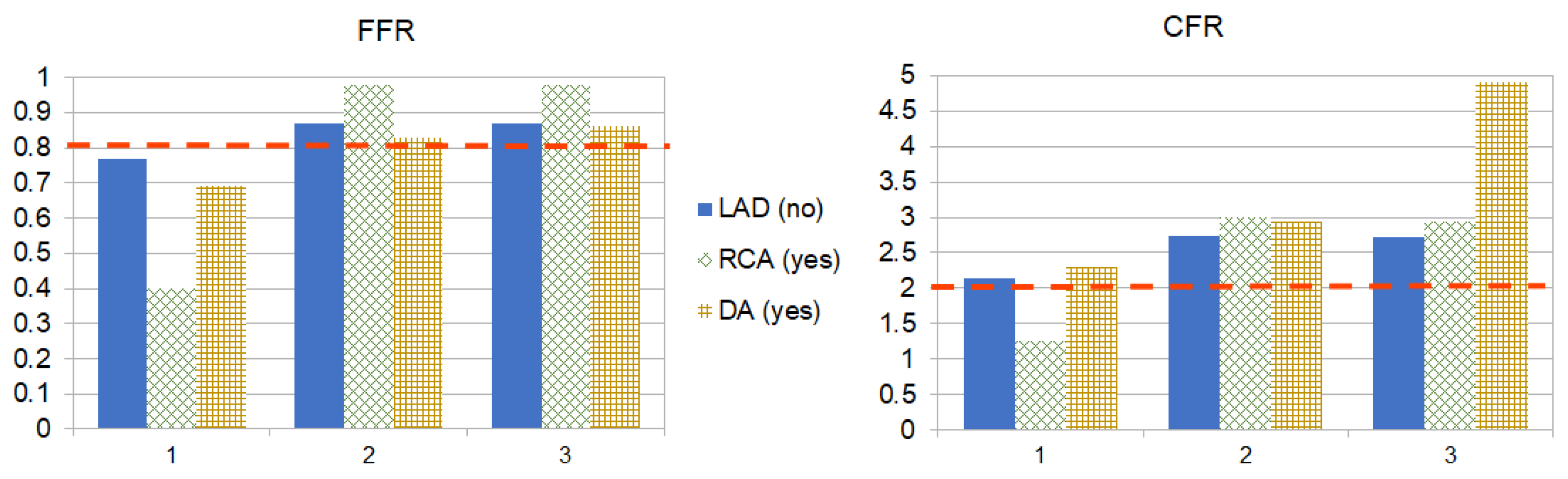
The computational domain for the model under consideration is represented by a 1D network of blood vessels. The network has to be connected in some way to the microcirculatory region of the myocardium. Coronary blood flow can be assessed both anatomically and functionally using myocardial CT perfusion (CTP) imaging. The technique enables the reconstruction of the anatomical structure of the coronary network, as well as an assessment of myocardial perfusion dysfunction. Several perfusion zones are identified in the myocardium. At least one of the terminal arteries of the 1D network has to be connected to each of the perfusion zones.

We have developed the following algorithm based on the CTP image to construct a personalized 1D network coupled with myocardial perfusion zones. It includes several stages: (1) preprocessing of CT and CTP images, (2) segmentation of the aortic root and ascending aorta, (3) left ventricular wall segmentation, (4) extraction of the structure of 1D vessels from CT images, (5) prescribing myocardial regions to each coronary artery, and (6) identification of model parameters.

The initial stage of the process involves cropping the computed tomography (CT) images in order to include both the left and right ventricular chambers. Additionally, the ascending aortae are sectioned between the aortic valve and the aortic arch (Figure 1). This step is essential for enhancing the detection of the aorta on the CT image. It also minimizes the computational burden of subsequent segmentation algorithms. In certain instances, it may be preferable to resample the voxels and make them more cubic in shape.

Step 2 involves the segmentation of the aorta in four main stages. First, the aorta is detected as the largest bright disc on the upper slice, using the circular Hough transform [26]. Secondly, the region that is most likely to be connected, centered around the seed point on the disc, is extracted as a preliminary estimation, utilizing the mean of the image intensities within the disc as a threshold parameter. Third, the initial guess is updated with the help of isoperimetric distance tree approach [27,28]. Finally, mathematical morphology operations [22] are used to smooth the segmented mask of the aorta.

In the third stage of the process, the myocardial wall is segmented using threshold-based techniques. The average intensity of myocardial wall voxels in computed tomography perfusion images is typically found to be in the range $[80;140]$ HU. The left ventricular wall, exhibiting heightened intensity values due to contrast enhancement, is situated adjacent to the left ventricular cavity. This wall can be distinguished from the atria by a plane that traverses the mitral valve. During segmentation, we prioritize identifying these boundaries, due to the notable change in intensity observed at their boundaries. We set all the extremely low intensities, all the negative intensities, and all the extremely high intensities to zero. The volume of the left ventricular wall is extracted as a contiguous region, encompassing the plane passing through the mitral valve (Figure 2). It is estimated that the position of the mitral valve plane is that plane which is perpendicular to the left ventricular axis and which passes through the interface between the right and left atrium.

In step 4, we use a Frangi filter [29] to detect coronary arteries. The initial seed locations are identified as the two voxels exhibiting the highest vesselness values on the aortic surface. The center lines of the coronary tree are then constructed using the distance-ordered homotopic thinning method [30]. The coronary tree is then partitioned into vessel segments, which results in a 1D coronary network suitable for mathematical calculations [22,28].

The presence of ischaemia may be indicated by the detection of a myocardial perfusion defect. TPR values characterize the flow of the microcirculation. They are provided by the CTP device for each voxel of the CTP image and are averaged over a standard set of 32 perfusion zones. There are two ways to perform TPR calculations. One is to use the original TPR values in the computations, or to truncate the TPR values to the range $[0.2,1]$, replacing all values below 0.2 with 0.2 and all values above 1 with 1. This restriction is introduced to reduce the impact of small TPR deviations.

In step 5, the ventricular wall is divided into individualized zones. Each zone is prescribed to a specific part of a previously constructed 1D coronary tree. Starting from the virtual root connecting the left and right coronary branches, the 1D network is then processed recursively. The ventricular wall is divided into several zones and the descending bifurcations are processed at each bifurcation point. Finally, the entire wall of the myocardium is divided into individual zones that correspond to the terminal arteries.

In this approach to the subdivision of a wall, the distance from the coronary arteries is taken into account. At the initial point of branching of the coronary artery, the artery is divided into two parts. The distances between each segment of the coronary arteries and each ventricular voxel are then calculated. These distances are then used to assign the voxels to the branch with the minimum distance by constructing zones where the distance to the selected branch is less than the distance to other branches.

The myocardial wall is divided into individual zones corresponding to the coronary segments by recursively descending through the coronary tree. As this process is carried out, the ventricle is partitioned, with only the part already belonging to the parent branch being taken. This is conducted in the same way at each branching point until the partitioned myocardial wall corresponding to the terminal segments of the coronary tree has been obtained (Figure 3).

Finally, in step 6, the TPR values of the individual zones are calculated as an average of the TPR values. As discussed above, in order to reduce confounding of local TPR values, the TPR values can be clipped prior to averaging

The above procedure was implemented as an independent C++ code on the basis of ITK library [31].

4. Results

For the personalization of blood flow models, a patient-specific evaluation of the pulse wave velocity, which defines the elastic properties of the coronary vessels [32], is required. We solve this problem using a feed-forward neural network (FFNN) trained on the synthetic database of simulated pulse waves [33,34] in a wide range of parameters. We use well-defined input parameters including age, HR (heart rate), SV (stroke volume), systolic, diastolic and mean blood pressures measured in the brachial artery. The details of the FFNN design and training have been described in detail in [35]. A similar FFNNs have been developed in [36,37]. Our FFNN predicts brachial-ankle AoPWV of real patients (102 patients from Sechenov University) with a mean square error of $1.3$ m/s and a relative standard deviation of $16\%$.

The objective of simulations utilizing the coronary blood flow model is to determine the pressure and flow within the coronary arteries as a function of space and time. Subsequently, a set of hemodynamic indices is calculated for each stenosis, in accordance with the following definitions.

Fractional flow reserve ($FFR$) is calculated as averaged over time blood pressure distal to stenosis (${\overline{P}}_{dist}^h$) divided by averaged over time proximal (aortic) pressure (${\overline{P}}_{aortic}^h$). FFR is measured during vasodilatation (hyperemia) [1]

$$FFR=\frac{{\overline{P}}_{dist}^h}{{\overline{P}}_{aortic}^h}.$$

(15)

The values of $FFR$ between 0.8 and 1.0 are indicative of a relatively mild stenosis. Values of $FFR$ below 0.8 may be considered as a possible indication for percutaneous coronary intervention (PCI).

Instantaneous wave-free ratio ($iFR$) is also the ratio between distal (${\overline{P}}_{dist}^w$) and proximal (${\overline{P}}_{aortic}^w$). However, pressure is averaged over the diastolic wave-free period (WFP) and hyperemia is not required [16].

$$iFR=\frac{{\overline{P}}_{dist}^w}{{\overline{P}}_{aortic}^w}.$$

(16)

We define WFP as a period between 25% of the way into diastole and the moment 5 ms before the end of cardiac cycle [3]. iFR also ranges between 0 and 1. The threshold value between significant and mild cases is 0.9.

Coronary flow reserve ($CFR$) is the ratio of the mean blood flow through a stenosed vessel during hyperemia (${\overline{Q}}^h$) to the average blood flow through the stenosed vessel under nonhyperemic normal condition (${\overline{Q}}^n$).

$$CFR=\frac{{\overline{Q}}^h}{{\overline{Q}}^n}.$$

(17)

$CFR$ is typically within the range of 1.0 to 4.0. Values greater than 3.0 are indicative of a healthy vessel. Values below 2.0 may be indicative of a potential indication for PCI.

We calculate all three indices ($FFR$, $CFR$, $iFR$) for three timeframes: before PCI, immediately after PCI and 2 to 3 months after PCI. We use CTP images and $TPR$ values before PCI to calculate the pre-treatment and post-treatment indices. We replace the occluded region with a healthy lumen in the second case. We assume that any microcirculatory impairment cannot be restored immediately after PCI, so we use the same $TPR$ values. We use CTP images and TPR values after PCI for the calculation of indices 2–3 months after treatment. They tell us how the lumen changed and how the microcirculatory regions changed.

We investigated a cohort of 11 patients. After admission to a hospital blood pressure, heart rate (HR) and stroke volume (SV) were measured. Blood pressure was measured with the cuff, stroke volume was measured by echocardiography and heart rate was obtained from ECG. Within two weeks first coronary CTP was performed. PCI was performed within a month after admission. Second coronary CTP was performed 2–3 months after PCI.

Table 1. Patient data. ID is the patient’s number; age is the patient’s age at the moment of first admission; sex is the patient’s sex (m—male, f—female); $P_{sys}$ is systolic pressure; $P_{dia}$ is diastolic pressure; $SV$ is stroke volume; $HR$ is heart rate.

ID	Age, Years	Sex	${\mathit{P}}_{\mathit{sys}}$, mmHg	${\mathit{P}}_{\mathit{dia}}$, mmHg	$\mathit{S}\mathit{V}$, mL	$\mathit{HR}$, bpm
1	73	m	140	80	47	85
2	67	m	130	80	82	80
3	49	f	135	72	56	78
4	57	m	120	70	73	80
5	60	f	120	80	72	60
6	62	m	130	80	83	70
7	70	m	140	80	65	84
8	70	m	135	81	33	89
9	68	f	120	70	53	62
10	56	m	107	76	35	64
11	50	m	120	75	93	57

briefly summarizes patients’ data. The structure of all 1D segmented networks and the full dataset can be found in Supplement Materials.

The simulation of stenosis entailed representing a distinguished vascular segment with a decreased diameter, in accordance with the patient data. We lower the terminal resistances by 70% [12,15] during hyperemia. In line with clinical observations during hyperemia, coronary blood flow increases 3–4 times.

We simulated six cases for each patient: before PCI at rest and during hyperemia, immediately after PCI at rest and during hyperemia, and long-term after PCI at rest and during hyperemia. Each case included CT segmentation for coronary network extraction, CTP segmentation and TPR value extraction and hemodynamic calculations. The case ‘immediately after PCI’ used the same segmentations as ‘before PCI’. CT segmentation was performed semi-automatically and took from 5 to 18 min for each case. CTP segmentation and TPR extraction took from 9 to 20 min and required a trained operator to perform. Hemodynamic calculations took from 2 to 5 min. All calculations were performed with a 1.7 GHz CPU with four cores and 8 Gb RAM.

Table 2. Calculated FFR, iFR, and CFR, hyperemic blood flow and rest blood flow. All values are calculated for three situations: before PCI, immediately after PCI, 3–6 months after PCI (long term). Letters ‘p’ and ‘d’ near the vessel name designate the proximal or distal part of the vessel, e.g., LADp—proximal part of LAD. ‘yes’ in parenthesis near the vessel name means that stenosis was stented, ‘no’—stenosis was not stented. Patients 1–5.

Patient 1
Vessel (stented)	Period	FFR	iFR	CFR
LADp (yes)	Before PCI	0.41 (0.43)	0.72	2.16
	After PCI	0.99	0.99	2.99
	Long term	0.98	0.99	2.72
Patient 2
Vessel (stented)	Period	FFR	iFR	CFR
RCA (no)	Before PCI	0.32	0.37	1.21
	After PCI	0.31	0.37	1.17
	Long term	0.24	0.23	1.25
LAD (yes)	Before PCI	0.80 (0.81)	0.81	2.18
	After PCI	0.99	0.99	2.61
	Long term	0.98	0.99	3.07
LCx (no)	Before PCI	0.20	0.29	1.13
	After PCI	0.19	0.29	1.14
	Long term	0.32	0.10	1.33
Patient 3
Vessel (stented)	Period	FFR	iFR	CFR
LAD (yes)	Before PCI	0.58 (0.58)	0.69 (0.53)	1.91
	After PCI	0.98	1.00	2.96
	Long term	0.99	1.00	2.91
LCx (yes)	Before PCI	0.56	0.58	1.83
	After PCI	0.98	1.00	3.01
	Long term	0.99	1.00	3.89
Patient 4
Vessel (stented)	Period	FFR	iFR	CFR
RCAp (no)	Before PCI	0.99	0.99	1.60
	After PCI	0.96	0.98	2.89
	Long term	0.96	0.97	2.94
RCAd (yes)	Before PCI	0.50	0.57 (0.56)	1.60
	After PCI	0.95	0.98	2.89
	Long term	0.96	0.98	2.94
LCx (no)	Before PCI	0.92	0.94	1.22
	After PCI	0.92	0.94	2.53
	Long term	0.89	0.95	2.55
DA (no)	Before PCI	0.70	0.86	1.38
	After PCI	0.70	0.86	2.14
	Long term	0.86	0.93	2.63
Patient 5
Vessel (stented)	Period	FFR	iFR	CFR
LAD (yes)	Before PCI	0.75	0.87	1.60
	After PCI	0.99	1.00	2.77
	Long term	0.96	0.99	3.05

,

Table 3. Calculated FFR, iFR, and CFR, hyperemic blood flow and rest blood flow. All values are calculated for three situations: before PCI, immediately after PCI, 3–6 months after PCI (long term). Letters ‘p’ and ‘d’ near the vessel name designate the proximal or distal part of the vessel, e.g., LADp—proximal part of LAD. ‘yes’ in parenthesis near the vessel name means that stenosis was stented, ‘no’—stenosis was not stented. Patients 6–9.

Patient 6
Vessel (stented)	Period	FFR	iFR	CFR
LAD (yes)	Before PCI	0.15	0.25	1.07
	After PCI	0.98	0.99	2.83
	Long term	0.88	0.95	2.35
RCA (no)	Before PCI	0.93 (0.94)	0.95	2.68
	After PCI	0.93	0.95	2.60
	Long term	0.95	0.96	2.84
OM (no)	Before PCI	0.75 (0.74)	0.91 (0.91)	2.42
	After PCI	0.75	0.91	2.34
	Long term	0.76	0.90	2.31
Patient 7
Vessel (stented)	Period	FFR	iFR	CFR
LAD (no)	Before PCI	0.76	0.95	1.71
	After PCI	0.76	0.96	2.10
	Long term	0.65	0.98	2.19
RCA (yes)	Before PCI	0.12	0.23	1.68
	After PCI	0.99	1.00	2.80
	Long term	0.98	0.99	3.01
LCx (yes)	Before PCI	0.11	0.38	1.82
	After PCI	0.99	0.99	3.70
	Long term	0.99	0.99	3.39
Patient 8
Vessel (stented)	Period	FFR	iFR	CFR
LAD (no)	Before PCI	0.77 (0.77)	0.86	2.14
	After PCI	0.87	0.95	2.74
	Long term	0.87	0.89	2.71
RCA (yes)	Before PCI	0.40	0.60	1.25
	After PCI	0.98	0.99	3.00
	Long term	0.98	0.99	2.95
DA (yes)	Before PCI	0.69 (0.69)	0.89	2.30
	After PCI	0.83	0.96	2.95
	Long term	0.86	0.93	4.9
Patient 9
Vessel (stented)	Period	FFR	iFR	CFR
LCx (yes)	Before PCI	0.64	0.74 (0.74)	1.9
	After PCI	0.99	0.99	2.75
	Long term	0.97	0.98	2.81
RCA (no)	Before PCI	0.91	0.96	2.95
	After PCI	0.96	0.96	2.92
	Long term	0.95	0.96	1.98
OM (no)	Before PCI	0.58	0.73	1.74
	After PCI	0.86	0.94	2.56
	Long term	0.88	0.95	2.74

and

Table 4. Calculated FFR, iFR, and CFR, hyperemic blood flow and rest blood flow. All values are calculated for three situations: before PCI, immediately after PCI, 3–6 months after PCI (long term). Letters ‘p’ and ‘d’ near the vessel name designate the proximal or distal part of the vessel, e.g., LADp—proximal part of LAD. ‘yes’ in parenthesis near the vessel name means that stenosis was stented, ‘no’—stenosis was not stented. Patients 10, 11.

Patient 10
Vessel (stented)	Period	FFR	iFR	CFR
OM (no)	Before PCI	0.91 (0.91)	0.96	1.98
	After PCI	0.91	0.96	1.96
	Long term	0.96	0.99	3.34
RCA (yes)	Before PCI	0.71 (0.71)	0.75	2.09
	After PCI	0.98 (0.98)	0.99	2.92
	Long term	0.97	0.99	3.16
Patient 11
Vessel (stented)	Period	FFR	iFR	CFR
LAD (yes)	Before PCI	0.52 (0.52)	0.66	1.66
	After PCI	0.93 (0.88)	0.98	2.71
	Long term	0.99	0.99	3.03
OM (yes)	Before PCI	0.41 (0.40)	0.66	1.50
	After PCI	0.93	0.98	2.81
	Long term	0.99	0.99	3.00

represent computed hemodynamic indices FFR, iFR, and CFR in the vessels with treated and untreated stenoses. The values in parentheses correspond to the invasive measurements. They are used to validate our model. By comparing the simulated and measured values in 17 cases, we obtained an average relative error of 3% with a standard mean deviation of 0.04.

The selection of vessels for treatment was determined by a physician based on the patient’s medical history, CT images, angiography, and measurements of FFR and iFR values.

Figure 4 shows correlations between FFR, iFR and CFR before treatment, immediately after treatment and long-term values. The correlation between FFR and iFR is high while CFR does not correlate well enough with either FFR or iFR, especially before treatment. Both FFR and iFR are pressure-based indices, whereas CFR is a flow-based index. Impaired perfusion and coronary vascular resistance have different effects on CFR and FFR/iFR [38]. While iFR and FFR can substitute each other, CFR and FFR/iFR are complementary. They can both contribute to better PCI guidance.

Graphic representation of Table 2, Table 3 and Table 4 helps to demonstrate the inevident effect of the multisite lesions caused by coronary hemodynamics. We selected patients 4 and 8 as the most representative examples. Similar graphs for all 11 patients can be found in Supplement Materials. Patient 8 had RCA and DA stented, which improved both FFR and CFR (Figure 5). The stenosis in LAD was not stented. However, both CFR and FFR improved significantly after PCI. This may be due to a compensatory effect of coronary blood flow. DA is a branch of LAD, but stenosis in LAD is located distal to the DA. Both LAD and DA supply areas of the myocardium that are close to each other. If one is stenosed, the volume of blood flowing through the other may increase to compensate for the loss of supply to the common areas of myocardium. After the DA was stented, blood flow through the DA increased and blood flow through the main branch of LAD decreased. As a result, the hemodynamic significance of LAD stenosis after PCI decreased and FFR/CFR improved.

Figure 6 shows a similar effect for patient 4. Here, we can observe a similar compensatory effect but in a more pronounced way. Patient 4 had RCA stented and it led to improvement in LCx and DA—the branches of LCA. In the previous case, we observed the interaction between two close branches of a single coronary artery—LAD. Here, PCI in RCA has affected a separate coronary artery—LCA. Some of the long-term improvements can be attributed to medications and non-surgical treatment. These factors can not explain short-term improvement.

Figure 7, Figure 8, Figure 9 and Figure 10 show confusion matrices for FFR, iFR, and CFR for 15 stenoses with invasively measured FFR or iFR. Stenosis is considered to be severe if invasive FFR < 0.8 or invasive iFR < 0.9. Calculated FFR is in perfect agreement with invasive measurements (Figure 7) with both sensitivity and specificity equal to 1.0. For calculated iFR sensitivity is 0.9 and specificity is 0.8 (Figure 8). This is due to the fact that the hemodynamic model presented has been adjusted to replicate pre-treatment measurements. The calculated CFR with a standard threshold of 2.0 does not effectively predict the hemodynamic significance of severe stenoses (Figure 9, sensitivity is 0.8 and specificity is 0.5). However, we can improve the specificity to 0.8 by slightly adjusting the threshold to 2.18 (Figure 10). This optimized threshold can be reasonably obtained from the ROC analysis of the CFR (Figure 11). We change the threshold to obtain the optimal values of sensitivity and specificity. CFR seems to be the least effective hemodynamic index in our analysis. This is due to the fact that the ground truth was based on invasive FFR and iFR measurements rather than CFR.

CFR can be very sensitive to the diameter of the arteries and to the structure of the vessels [14]. The absence of one single artery causes a redistribution of blood flow that affects CFR values. Healthy CFR values can vary from 2.0 to 5.0 for different patients [39]. Unlike FFR or iFR, a single threshold value for CFR does not usually work for all patients. It is difficult to compare the CFR of different patients, but we can compare changes in CFR values before and after treatment.

One of the interesting observations is that CFR increases after PCI but does not return to a healthy value immediately (above 3.0). Simulations for the long-term conditions show that in most cases CFR steadily grows during the postoperative period. The average value of CFR for treated vessels after the PCI is 2.91 and it grows to 3.02 (Figure 12). The long-term CFR is higher than the post-treatment CFR. CFR index characterizes the ability of the coronaries to increase blood flow under stress. Long-term increases in CFR can be caused by the improvement of myocardial perfusion due to stenosis removal. We assume that immediately after PCI, perfusion is still hindered, and it takes time for it to improve.

5. Discussion

In some previous works, we confirm that the 1D hemodynamical model is able to estimate FFR with the same accuracy as instrumental invasive measurements and patient-specific sensitivity based on non-invasively collected data. Based on our computational results, we conclude that TPR data on myocardial perfusion improve the accuracy of FFR, iFR, and CFR estimations and provide a better understanding of stenoses severity. We achieve an average relative error of 3% with a standard mean deviation of 0.04. The previous works ignoring the state of myocardial perfusion provide the error 5–11% [15,40,41,42,43].

FFR and iFR are strongly correlated at all stages of treatment including before PCI, after PCI and in the long term. This means that only iFR or only FFR could be measured for diagnosis. The iFR measurements do not require vasodilation and, thus, have fewer side effects. FFR is better studied and considered to be a ’golden standard’. We did not find any significant discrepancies between FFR and iFR predictions. The difference between FFR and iFR can still be observed in in-patients with aortic valve diseases [44] and probably in other pathological cases. Thus, some research recommends using both indices [45]. Our approach allows the evaluation of all hemodynamic indicators based on non-invasive data with high accuracy.

Both FFR and iFR correlated poorly with CFR before PCI treatment and correlated strongly with CFR at all stages after the treatment. The miscorrelation before PCI may be due to two reasons. Firstly, there may be an insufficient number of available measurements, which prevents proper validation of the model. Secondly, there may be a substantially different relationship between pressure and flow in the presence of stenosis. For instance, previous studies have shown [46] that vessels with different diameters and the same degree of stenosis have different FFRs, while the flow and, thus, CFR depends on the lumen. Further investigation is required to confirm this hypothesis.

Our computational results show that PCI increases the FFR, the iFR and the CFR in the coronary arteries in both the short and the long term. It is noteworthy that PCI of stenosis also increases the values of hemodynamic indices in neighboring vessels with stenoses, with the effect being more pronounced in the long term. This fact is demonstrated in Figure 5 and Figure 6 and was observed in a lot of other cases. We associate the short-term effect immediately after PCI with the compensation, which results in a flow and pressure decrease in the neighboring vessels with stenoses. In the long-term period, an additional positive factor is myocardial perfusion recovery. It causes a decrease in terminal hydraulic resistance for a group of arteries including treated and untreated.

The developed model can be used for clinical diagnostics based on FFR and iFR analysis. Figure 7 and Figure 8 demonstrate the diagnostic accuracy, which is similar to the other works based on 3D simulations [47]. We achieve our result much faster using an advanced 1D approach. We note that we considered just 11 patients and 15 stenoses. Obviously, the model should be thoroughly tested on a much larger cohort of patients. After thorough testing proposed approach can be used to estimate the hemodynamic significance of stenoses or perfusion impairments. In real cases, patients may have multiple lesions and regions with myocardial dysfunction. Interactions between these pathologies are complex and the choice of treatment may depend on many factors. A well-tuned coronary hemodynamic model allows us to ‘turn off’ some of the pathologies and evaluate the impact of each separate stenosis and each region with impaired perfusion. This approach could also help to better match regions with impaired perfusion with supplying coronary arteries.

Unsatisfactory diagnosis based on CFR is related to the lack of direct measurements of flow, high individual variability of threshold, and high sensitivity of CFR to arterial diameter and vessel structure. We use an ROC curve to adjust the threshold for CFR. This gives a better predictive power. However, it cannot be considered as a final solution to the problem.

Some technical problems limit our work. First, we note that insufficient quality of CT data leads to defects in vessel structure. In fact, the segmentation procedure provides different structures even for the same patient after a short period of time (e.g., before and after PCI). To address this issue, we utilize a previously developed algorithm for identifying terminal resistance [21], which reduces sensitivity to incomplete structure recognition. In addition, a customised perfusion zone generation algorithm is used to segment the myocardial surface according to the presence of terminal vessels after segmentation. Secondly, there is no clear relationship between TPR values and terminal hydraulic resistance. In our work, we used an empirical function. The other possibility is the use of complex models of myocardial microcirculation.

References

1. Pijls, N.H.J.; de Bruyne, B.; Peels, K.; van der Voort, P.H.; Bonnier Hans, J.R.M.; Bartunek, J.; Koolen, J.J. Measurement of Fractional Flow Reserve to Assess the Functional Severity of Coronary-Artery Stenoses. N. Engl. J. Med. 1996, 334, 1703–1708. [Google Scholar] [CrossRef]
2. Gould, K.L.; Kirkeeide, R.L.; Buchi, M. Coronary flow reserve as a physiologic measure of stenosis severity. J. Am. Coll. Cardiol. 1990, 15, 459–474. [Google Scholar] [CrossRef]
3. Sen, S.; Escaned, J.; Malik, I.S.; Mikhail, G.W.; Foale, R.A.; Mila, R.; Tarkin, J.; Petraco, R.; Broyd, C.; Jabbou, R.; et al. Development and validation of a new adenosine–independent index of stenosis severity from coronary wave-intensity analysis: Results of the ADVISE (ADenosine Vasodilator Independent Stenosis Evaluation) study. J. Am. Coll. Cardiol. 2012, 59, 1392–1402. [Google Scholar] [CrossRef]
4. Seitun, S.; De Lorenzi, C.; Cademartiri, F.; Buscaglia, A.; Travaglio, N.; Balbi, M.; Bezante, G.P. CT Myocardial perfusion imaging: A new frontier in cardiac imaging. BioMed Res. Int. 2018, 2018, 7295460. [Google Scholar] [CrossRef]
5. Zaman, M.M.; Haque, S.S.; Siddique, M.A.; Banerjee, S.; Ahmed, C.M.; Sharma, A.K.; Rahman, M.F.; Haque, M.H.; Joarder, A.I.; Sultan, A.U.; et al. Correlation between severity of coronary artery stenosis and perfusion defect assessed by SPECT myocardial perfusion imaging. Mymensingh Med. J. 2010, 19, 608–613. [Google Scholar] [PubMed]
6. Camici, P.G.; Magnoni, M. How important is microcirculation in clinical practice? Eur. Heart. J. Suppl. 2019, 21, B25–B27. [Google Scholar] [CrossRef] [PubMed]
7. Sambuceti, G.; L’Abbate, A.; Marzilli, M. Why should we study the coronary microcirculation? Am. J.-Physiol.-Heart Circ. Physiol. 2000, 279, H2581–H2584. [Google Scholar] [CrossRef]
8. George, R.T.; Arbab-Zadeh, A.; Miller, J.M.; Kitagawa, K.; Chang, H.J.; Bluemke, D.A.; Becker, L.; Yousuf, O.; Texter, J.; Lardo, A.C.; et al. Adenosine stress 64- and 256-row detector computed tomography angiography and perfusion imaging: A pilot study evaluating the transmural extent of perfusion abnormalities to predict atherosclerosis causing myocardial ischemia. Circ. Cardiovasc. Imaging 2009, 2, 174–182. [Google Scholar] [CrossRef] [PubMed]
9. Cury, R.C.; Magalhães, T.A.; Paladino, A.T.; Shiozaki, A.A.; Perini, M.; Senra, T.; Lemos, P.A.; Rochitte, C.E. Dipyridamole stress and rest transmural myocardial perfusion ratio evaluation by 64 detector-row computed tomography. J. Cardiovasc. Comput. Tomogr. 2011, 5, 443–448. [Google Scholar] [CrossRef]
10. Coenen, A.; Rossi, A.; Lubbers, M.M.; Kurata, A.; Kono, A.K.; Chelu, R.G.; Segreto, S.; Dijkshoorn, M.L.; Wragg, A.; van Geuns, R.-J.M.; et al. Integrating CT Myocardial Perfusion and CT-FFR in the Work-Up of Coronary Artery Disease. JACC Cardiovasc. Imaging 2017, 10, 760–770. [Google Scholar] [CrossRef]
11. Ihdayhid, A.R.; Sakaguchi, T.; Linde, J.J.; Sørgaard, M.H.; Kofoed, K.F.; Fujisawa, Y.; Hislop-Jambrich, J.; Nerlekar, N.; Cameron, J.D.; Munnur, R.K.; et al. Performance of computed tomography-derived fractional flow reserve using reduced-order modelling and static computed tomography stress myocardial perfusion imaging for detection of haemodynamically significant coronary stenosis. Eur. Heart J. Cardiovasc. Imaging 2018, 19, 1234–1243. [Google Scholar] [CrossRef] [PubMed]
12. Lo, E.W.; Menezes, L.J.; Torii, R. On outflow boundary conditions for CT-based computation of FFR: Examination using PET images. Med. Eng. Phys. 2020, 76, 79–87. [Google Scholar] [CrossRef]
13. Simakov, S.; Gamilov, T.; Liang, F.; Gognieva, D.G.; Gappoeva, M.K.; Kopylov, P.Y. Numerical evaluation of the effectiveness of coronary revascularization. Russ. J. Numer. Anal. Math. Model. 2021, 36, 303–312. [Google Scholar] [CrossRef]
14. Ge, X.; Liu, Y.; Tu, S.; Simakov, S.; Vassilevski, Y.; Liang, F. Model-based analysis of the sensitivities and diagnostic implications of FFR and CFR under various pathological conditions. Int. J. Numer. Methods Biomed. Eng. 2019, 37, e3257. [Google Scholar] [CrossRef] [PubMed]
15. Carson, J.M.; Pant, S.; Roobottom, C.; Alcock, R.; Blanco, P.J.; Carlos Bulant, C.A.; Vassilevski, Y.; Simakov, S.; Gamilov, T.; Pryamonosov, R.; et al. Non-invasive coronary CT angiography-derived fractional flow reserve: A benchmark study comparing the diagnostic performance of four different computational methodologies. Int. J. Numer. Methods Biomed. Eng. 2019, 35, e3235. [Google Scholar] [CrossRef] [PubMed]
16. Carson, J.M.; Roobottom, C.; Alcock, R.; Nithiarasu, P. Computational instantaneous wave-free ratio (IFR) for patient-specific coronary artery stenoses using 1D network models. Int. J. Numer. Methods Biomed. Eng. 2019, 35, e3255. [Google Scholar] [CrossRef]
17. Gamilov, T.M.; Kopylov, P.Y.; Pryamonosov, R.A.; Simakov, S.S. Virtual fractional flow reserve assessment in patient-specific coronary networks by 1D haemodynamic model. Russ. J. Numer. Anal. Math. Model. 2015, 30, 269–276. [Google Scholar] [CrossRef]
18. Lu, M.T.; Ferencik, M.; Roberts, R.S.; Lee, K.L.; Ivanov, A.; Adami, E.; Mark, D.B.; Jaffer, F.A.; Leipsic, J.A.; Douglas, P.S.; et al. Noninvasive FFR Derived From Coronary CT Angiography: Management and Outcomes in the PROMISE Trial. JACC Cardiovasc. Imaging 2017, 10, 1350–1358. [Google Scholar] [CrossRef]
19. Feng, Y.; Ruisen, F.; Li, B.; Li, N.; Yang, H.; Liu, J.; Liu, Y. Prediction of fractional flow reserve based on reduced-order cardiovascular model. Comput. Methods Appl. Mech. Eng. 2022, 400, 115473. [Google Scholar] [CrossRef]
20. Gamilov, T.; Kopylov, P.; Serova, M.; Syunyaev, R.; Pikunov, A.; Belova, S.; Liang, F.; Alastruey, J.; Simakov, S. Computational analysis of coronary blood flow: The role of asynchronous pacing and arrhythmias. Mathematics 2020, 8, 1205. [Google Scholar] [CrossRef]
21. Simakov, S.; Gamilov, T.; Liang, F.; Kopylov, P. Computational analysis of haemodynamic indices in synthetic atherosclerotic coronary netwroks. Mathematics 2021, 9, 2221. [Google Scholar] [CrossRef]
22. Vassilevski, Y.; Olshanskii, M.; Simakov, S.; Kolobov, A.; Danilov, A. Personalized Computational Hemodynamics. Models, Methods, and Applications for Vascular Surgery and Antitumor Therapy, 1st ed.; Academic Press: Cambridge, MA, USA, 2020. [Google Scholar]
23. Vassilevski, Y.V.; Salamatova, V.Y.; Simakov, S.S. On the elasticity of blood vessels in one-dimensional problems of haemodynamics. Comput. Math. Math. Phys. 2015, 55, 1567–1578. [Google Scholar] [CrossRef]
24. Coenen, A.; Lubbers, M.M.; Kurata, A.; Kono, A.; Dedic, A.; Chelu, R.G.; Dijkshoorn, M.L.; Rossi, A.; van Geuns, R.M.; Nieman, K. Diagnostic value of transmural perfusion ratio derived from dynamic CT-based myocardial perfusion imaging for the detection of haemodynamically relevant coronary artery stenosis. Eur. Radiol. 2017, 27, 2309–2316. [Google Scholar] [CrossRef] [PubMed]
25. Magomedov, K.M.; Kholodov, A.S. Grid–Characteristic Numerical Methods; Nauka: Moscow, Russia, 2018. (In Russian) [Google Scholar]
26. Duda, R.O.; Hart, P.E. Use of the Hough transformation to detect lines and curves in pictures. Commun. Acm 1972, 15, 11–15. [Google Scholar] [CrossRef]
27. Grady, L.K. Fast, quality, segmentation of large volumes—Isoperimetric distance trees. In Computer Vision—ECCV 2006; Springer: Berlin/Heidelberg, Germany, 2006; pp. 449–462. [Google Scholar]
28. Danilov, A.; Ivanov, Y.; Pryamonosov, R.; Vassilevski, Y. Methods of graph network reconstruction in personalized medicine. Int. J. Num. Met. Biomed. Engn. 2015, 32, e02754. [Google Scholar] [CrossRef] [PubMed]
29. Frangi, A.F.; Niessen, W.J.; Vincken, K.L.; Viergever, M.A. Multiscale vessel enhancement filtering. In Medical Image Computing and Computer-Assisted Intervention—MICCAI’98; Springer: Berlin/Heidelberg, Germany, 1998; pp. 130–137. [Google Scholar]
30. Pudney, C. Distance-ordered homotopic thinning: A skeletonization algorithm for 3D digital images. Comput. Vis. Image Underst. 1998, 72, 404–413. [Google Scholar] [CrossRef]
31. McCormick, M.; Liu, X.; Jomier, J.; Marion, C.; Ibanez, L. ITK: Enabling reproducible research and open science. Front. Neuroinform. 2014, 8, 13. [Google Scholar] [CrossRef] [PubMed]
32. Sugawara, J.; Hayashi, K.; Yokoi, T.; Cortez-Cooper, M.Y.; DeVan, A.E.; Anton, M.A.; Tanaka, H. Brachial–ankle pulse wave velocity: An index of central arterial stiffness? J. Hum. Hypertens 2005, 19, 401–406. [Google Scholar] [CrossRef] [PubMed]
33. Charlton, P.H.; Mariscal Harana, J.; Vennin, S.; Li, Y.; Chowienczyk, P.; Alastruey, J. Modeling arterial pulse waves in healthy aging: A database for in silico evaluation of hemodynamics and pulse wave indexes. Am. J.-Physiol. Circ. Physiol. 2019, 317, H1062–H1085. [Google Scholar] [CrossRef]
34. Charlton, P.H. Pulse Wave Database. Available online: https://peterhcharlton.github.io/pwdb/pwdb.html (accessed on 31 March 2024).
35. Gamilov, T.; Liang, F.; Kopylov, P.; Kuznetsova, N.; Rogov, A.; Simakov, S. Computational analysis of hemodynamic indices based on personalized identification of aortic pulse wave velocity by a neural network. Mathematics 2023, 11, 1358. [Google Scholar] [CrossRef]
36. Jin, W.; Chowienczyk, P.; Alastruey, J. Estimating pulse wave velocity from the radial pressure wave using machine learning algorithms. PLoS ONE 2021, 16, e0245026. [Google Scholar] [CrossRef] [PubMed]
37. Tavallali, P.; Razavi, M.; Pahlevan, N.M. Artificial Intelligence Estimation of Carotid-Femoral Pulse Wave Velocity using Carotid Waveform. Sci. Rep. 2018, 8, 1014. [Google Scholar] [CrossRef] [PubMed]
38. Garcia, D.; Harbaoui, B.; van de Hoef, T.P.; Meuwissen, M.; Nijjer, S.S.; Echavarria-Pinto, M.; Davies, J.E.; Piek, J.J.; Lantelme, P. Relationship between FFR, CFR and coronary microvascular resistance—Practical implications for FFR-guided percutaneous coronary intervention. PLoS ONE 2019, 14, e0208612. [Google Scholar] [CrossRef] [PubMed]
39. Fearon, W.F. 14—Invasive Testing. In Chronic Coronary Artery Disease; de Lemos, J.A., Omland, T., Eds.; Elsevier: Amsterdam, The Netherlands, 2018; pp. 194–203. [Google Scholar]
40. Morris, P.D.; Ryan, D.; Morton, A.C. Virtual fractional flow reserve from coronary angiography: Modeling the significance of coronary lesions: Results from the VIRTU-1 (VIRTUal Fractional Flow Reserve from Coronary Angiography) study. JACC Cardiovasc. Interv. 2013, 6, 149–157. [Google Scholar] [CrossRef]
41. Tu, S.; Barbato, E.; Köszegi, Z.; Yang, J.; Sun, Z.; Holm, N.R.; Tar, B.; Li, Y.; Rusinaru, D.; Wijns, W.; et al. Fractional flow reserve calculation from 3 to dimensional quantitative coronary angiography and TIMI frame count: A fast computer model to quantify the functional significance of moderately obstructed coronary arteries. JACC Cardiovasc. Interv. 2014, 7, 768–777. [Google Scholar] [CrossRef] [PubMed]
42. Koo, B.-K.; Erglis, A.; Doh, J.-H.; Daniels, D.V.; Jegere, S.; Kim, H.-S.; Dunning, A.; DeFrance, T.; Lansky, A.; Leipsic, J.; et al. Diagnosis of Ischemia-Causing Coronary Stenoses by Noninvasive Fractional Flow Reserve Computed from Coronary Computed Tomographic Angiograms: Results from the Prospective Multicenter DISCOVER-FLOW (Diagnosis of Ischemia-Causing Stenoses Obtained Via Noninvasive Fractional Flow Reserve) Study. JACC 2011, 58, 1989–1997. [Google Scholar] [PubMed]
43. Nakazato, R.; Park, H.-B.; Berman, D.S.; Gransar, H.; Koo, B.-K.; Erglis, A.; Lin, F.Y.; Dunning, A.M.; Budoff, M.J.; Malpeso, J.; et al. Noninvasive fractional flow reserve derived from computed tomography angiography for coronary lesions of intermediate stenosis severity. Circ. Cardiovasc. Imaging 2013, 6, 881–889. [Google Scholar] [CrossRef] [PubMed]
44. Ge, X.; Liu, Y.; Yin, Z.; Tu, S.; Fan, Y.; Vassilevski, Y.; Simakov, S.; Liang, F. Comparison of instantaneous wave-free Ratio (iFR) and fractional flow reserve (FFR) with respect to their sensitivities to cardiovascular factors: A computational model-based study. J. Interv. Cardiol. 2020, 2020, 4094121. [Google Scholar] [CrossRef]
45. Kern, M.J.; Seto, A.H. Vive la difference: Factors and mechanisms predicting discrepancy between iFR and FFR. Catheter. Cardiovasc. Interv. 2019, 94, 364–366. [Google Scholar] [CrossRef] [PubMed]
46. Simakov, S.S.; Gamilov, T.M.; Kopylov, F.Y.; Vasilevskii, Y.V. Evaluation of Hemodynamic Significance of Stenosis in Multiple Involvement of the Coronary Vessels by Mathematical Simulation. Bull. Exp. Biol. Med. 2016, 162, 111–114. [Google Scholar] [CrossRef]
47. Morris, P.D.; van de Vosse, F.N.; Lawford, P.V.; Hose, D.R.; Gunn, J.P. “Virtual” (Computed) Fractional Flow Reserve: Current Challenges and Limitations. JACC Cardiovasc. Interv. 2015, 8, 1009–1017. [Google Scholar] [CrossRef] [PubMed]
Figure 1. A section of a CTP image showing high contrast in the ventricles, moderate intensity in the myocardial wall and low intensity in the surrounding tissue.
Computation 12 00110 g001
Figure 2. Segmentation of the aorta and left ventricle walls for CTP image: aorta in red color, left ventricle walls in green color.
Computation 12 00110 g002
Figure 3. Final partitioning of the left ventricle wall with supplying coronary arteries (the same color as a segment) and aorta (shown in red).
Computation 12 00110 g003
Figure 4. Correlation between FFR, iFR and CFR.
Computation 12 00110 g004
Figure 5. FFR and CFR for patient No. 8. The red dashed line indicates the threshold between healthy and pathological cases.
Computation 12 00110 g005
Figure 6. FFR and CFR for patient No. 4. The red dashed line indicates the threshold between healthy and pathological cases.
Computation 12 00110 g006
Figure 7. Confusion matrix for calculated FFR. Specificity is 1.0 and sensitivity is 1.0.
Computation 12 00110 g007
Figure 8. Confusion matrix for calculated iFR. Specificity is 0.8 and sensitivity is 0.9.
Computation 12 00110 g008
Figure 9. Confusion matrix for calculated CFR with threshold 2.0. Specificity is 0.8 and sensitivity is 0.5.
Computation 12 00110 g009
Figure 10. Confusion matrix for calculated CFR with threshold 2.18. Specificity is 0.8 and sensitivity is 0.8.
Computation 12 00110 g010
Figure 11. ROC curve for calculated CFR. Optimal value for CFR threshold (2.18) was chosen by minimizing the distance between the ROC curve and point (0.0; 1.0).
Computation 12 00110 g011
Figure 12. Calculated CFR before PCI, after PCI and long term values.
Computation 12 00110 g012