The Effect of Critical Distance in Digital Levelling

Abstract

Critical distance concerns precise digital levelling, which has inaccurate results at a certain sighting distance. The influence of critical distance on a measured height difference has been confirmed by calibrating certain digital levels and their appropriate code devices on a vertical comparator under laboratory conditions. The paper aims to explore the influence of critical distance on height differences obtained by precise digital levels of Leica NA3003 and DNA03 by experimental measurements realised in situ. The processing of the measurement results consisted of defining a random error on a station by using parameter estimation of an error model to specify a partial error on a station dependent on sighting distance. Then the processing phase continues with the finding of the relation between the sighting distance and the dispersion of height differences acquired by digital levelling under terrain conditions. The theoretical part involves the development of levelling accuracy theories that vary over time by view on random and systematic error propagation. The numerical and graphical solution of the experimental measurements involves ordering the height differences into sighting groups according to the sighting distance. The standard deviation computed in each sighting group represents a measure of the dispersion of height differences. Suppose the standard deviation in the sighting group in both independent experimental locations K1 and K2 exceeds twice the total standard deviation. In that case, it is most likely considered to be the influence of the critical distance, which is then compared with values obtained by laboratory calibration of the same digital levels.

1. Introduction

Digital levelling in engineering geodesy brings quick, precise and reliable measurements, often performed under real industrial or building discomfort conditions. The present experience from diagnostics of transport constructions realised by digital levels has brought increased occurrence of levelling errors in some cases. This problem and knowledge of the existence of critical sighting distance of specific digital levels demonstrated by Gassner and Rulland in [1,2] have started research aimed at finding the probable effect of this anomaly on the precision of height differences measured at various sighting distances. Moreover, mathematical modelling involved in the data processing should bring the view of the levelling error sources on a station and determine the ratio between errors dependent and independent of sighting distance.

Accuracy analysis of precise levelling is a highly developed theme by many researchers, who devoted their research to the calibration of the levelling system. For example, Baričevič and his colleagues [3] devoted their research to the automatic calibration of levelling staff, Kuchmister with his co-authors [4] describe the functionality of a vertical comparator based on an interferometric measuring system built in a laboratory at Wroclaw University, Takalo and Rouhiainen [5] from the Finnish Geodetic Institute describe a calibration system based on two concrete pillars for Zeiss DiNi instruments and a vertical laser system for rod testing and Woschitz and his colleagues describe the vertical comparator developed at Graz University in [6,7,8]. Authors such as Rekus [9], Sjoberg [10], Yaprak [11], Zilkovski [12] and others have focused their research on accuracy performance and analysis of systematic and random levelling errors. Though the mentioned authors do not directly devote their research to the influence of critical sighting distance, their approach to the accuracy analysis was inspirative for the presented methodology. A short overview of the references concerning the analysis of digital levelling systems is in the second section of this paper. The difference between the presented research and those that are published in the cited references is in organising the special experimental measurements to find the effect of the critical sighting distance on levelling accuracy by using specific digital levels applied under various atmospheric conditions in various seasons. The reliability of the used methodology was verified by comparing the results from two independent localities.

The critical sighting distance should be caused by the systematic effect on measured height differences, therefore the research described in the paper consists of accuracy analysis of levelling data, which is based on classical theories of accuracy, which over time have adapted to new knowledge and technologies and brought a new representation of random and systematic components. The process of investigating the influence of the critical sighting distance consisted of an accuracy analysis of the height differences in the fixed points stabilised in situ on the concrete structure. The particular points have been measured by precise digital levels NA3003 and DNA3, each in four measurement cycles. The experimental measurements were organized into two independent levelling routes with a length of 0.500 km, while the length of intermediate sight on fixed points varied from 2 m to 35 m. The paper deals with a levelling error analysis to detect the partial errors that appeared as a sum of elementary errors accumulated on each station to differentiate errors dependent on the sighting distance. The total levelling error is composed of elementary errors accumulated in each backsight and foresight of a station. The main characteristics of accuracy respect this fact and involve the number of levelling stations, sighting distances and the measured height differences as main arguments in their formulas. Levelling error analysis is based on the basic formulas recommended by the International Association of Geodesy (IAG), which have been subjected to new views on the propagation of random and systematic errors over time. The current error analysis methods respect digital technologies, which brought new errors and changed the ratio of random and systematic error propagation [13]. The well-established method of finding the influence of elementary errors in observed levelling data consists of parameter estimation of a mathematical model created from the components of levelling errors, which are (in)dependent on the sighting distance. The model estimations vary in each station, but the discrepancy in their numerical order should be the same. If not, suspicions of the influence of systematic error on a levelling station appear. Then the weighted standard deviations were computed for each meter of sighting distance, named sighting groups, to find the relationship between the height differences dispersion and the sighting distance to find the possible influence of critical distance for the specific digital level. Critical distance is a well-known term among geodesists and metrologists who know that a high probability of obtaining inaccurate results appears at a certain sighting distance during digital levelling. The existence of this critical distance on specific digital levels has been confirmed by calibrating levelling devices at the vertical comparator. As we have the values of critical distances of Leica levelling devices published in [1,2], we can compare the results of field measurements with theoretical values.

2. An Overview of Levelling Error Theories

One of the first official theories concerning levelling error propagation was presented by Ch. Lallemand, a French geophysicist and the first president of the International Union of Geodesy and Geophysics. He separated random and systematic influence in levelling measurements and defined international valid tolerances for comparing levelling accuracy in other countries (Bulletin géodésique 1930). In 1912, the Union accepted his theory and registered the official formulas for analysing levelling accuracy. Later, G. A. Rune tried to improve the Lallemand equations by estimating levelling standard deviation as a quadratic difference between the total and random error (Zeitschrift für Vermessungswesen 1930). The head of the French Institut Géographique National in Paris J. Vignal has brought a new view on systematic errors in levelling that influence measurements up to a certain length, and after exceeding it, their variable influence is similar to the behaviour of random errors. After some objections from a member of the Finnish Academy of Sciences, T. J. Kukkamäki and J. Vignal modified his theories, which were subsequently accepted by the Geodetic Union in Oslo. J. Bohm and J. Sloboda summarised the existing theories of levelling error propagation in their book [14].

Over time, views on accuracy analysis and levelling error propagation have adapted to technological improvements in levelling instruments and their accessories. L. Sjöberg published a professional paper [10] concerning the influence of systematic and random errors on the precision of one-way levelling routes measured by a motorised technique. M. Craymer published a thesis [15] devoted to the analysis of Swiss levelling measurements from the point of systematic effects. P. Vaníček and M. Craymer devoted their research to the rod settlement effect on levelling precision [16]. D. Zilkovski applied a “special adjustment” of levelling data based on using preliminary errors in evaluating levelling results that were published in [12]. Rekus [9] and Saaranen [17] analysed robotized digital levelling in its practical applications. Yaprack [11] and Cvetkov [18] devoted their research to digital level applications in precise height systems. Besides field measurements, technological progress and automation also affected the calibration process of levelling systems. The authors H. Woschitz and F. Brunner described in [6,7,8] the calibration facilities and outcomes from testing certain digital levels at the Laboratory of Geodetic Metrology of the Graz University of Technology (TUG). The conception of the TUG vertical comparator inspired the construction of the calibration system at the Stanford Linear Accelerator Center (SLAC). The authors Gassner and Ruland presented in [1,2] the hardware and experimental results of the SLAC calibration system used to test levelling invar rods of the levelling devices Leica NA3003, DNA03, and Trimble DiNi12. Baričevič and his colleagues [3] also devoted their research to the calibration levelling staff by presenting a new calibration system. Interesting results concerning digital level calibration brought Takalo [5], Kuchmister [4] and Elhassan et al. [19] with their comparison of indoor and outdoor levelling accuracy of digital and optical levels.

3. Basic Formulas for an Analysis of Levelling Accuracy

The accuracy analysis of levelling data consists of applying well-known formulas, which have been adapted to new levelling technologies to bring a new perspective on the representation of the random and systematic components. The basic formulas of classical accuracy theories are based on defining the sources of levelling errors, the representation of the components of random and systematic influences and the theory of error propagation. Lallemand differentiated the terms random and systematic error in levelling measurement and estimated the variable systematic errors from the cumulative frequency of two levelling routes. The estimation process was based on a hypothesis that assumes an upward or downward tendency of linear regression, possibly caused by the systematic effect. His theory of accuracy is based on the height differences in bidirectional levelling adjusted to the length of one kilometre of the levelling route. The reliable estimation of the accuracy of a one-kilometre-long levelling route is derived by using the law of error propagation of levelling errors. It is given by the quadratic mean of double levelling, known as unit standard deviation. Lallemand recalculated height differences in two-way levelling on kilometre differences by dividing by root squared of the quantity R, representing the length of the levelling route in km. Then the most used accuracy estimation of a one-kilometre-long levelling route follows from the law of error propagation and is given by the quadratic mean of double levelling. This accuracy characteristic is known as the unit standard deviation σ₀ and is given by the following formula [14]:

$${\sigma }_0=\frac{1}{2}\sqrt{\frac{1}{n_R}{\displaystyle \sum \frac{{\rho }^2}{R}}},$$

(1)

where ρ is the difference between height differences computed in each direct and reverse levelling section with length R given in kilometres. Over time, the restrictive conditions for the universal use of Lallemand formulas appear. His main opponent was Vignal, whose theory consisted of a determination of a limited length of the levelling route, within which unit standard deviation presented in Formula (1) includes only the effect of random errors and short-periodical variable systematic ones. Other levelling lines that exceed the limited length contain also long-periodic systematic errors, which influence levelling observations with the same sign, so they need not be eliminated by bidirectional levelling. The Vignal theory for accuracy analysis of precise levelling is based on the following statements:

• Lallemand’s deviations of the cumulative height differences in bidirectional levelling are caused not only by systematic errors but also by random noise.
• The influence of systematic errors defined by Lallemand is valid only within a certain distance (limited length) of the levelling route, beyond which they behave as variable systematic errors dispersed around the mean systematic error.
• Levelling variance is expressed as a root square of the total variance:

$${\tau }^2={\eta }^2+{\xi }^2.$$

(2)

The quantity represents a random and systematic component with variable behaviour in the frame of limit length and beyond, and it behaves as a constant. The systematic influence can be calculated according to the following equation [20]:

$$\xi =\zeta \frac{K}{Z}{R}_m,$$

(3)

where K is a constant equal to 2 or 3, Z is the limit length and R_m is the mean distance of the levelling sections. The value ζ can be determined from the levelling closures or using differences in the endpoints of the regression line, estimated from the cumulative differences in the height difference in bidirectional levelling in the levelling sections.

Assuming n stations in the levelling route, the total variance is equal to the following relationship [9,14,21]:

$${\sigma }^2=n{\eta }^2+n^2{\xi }^2.$$

(4)

Random errors η in the levelling route increase in proportion to the number of stations, and the occurrence of systematic error ξ depends on the square of the number of stations. The behaviour of the random and systematic component varies in the frame of limit length, and beyond, it behaves as a constant. The systematic components can be determined from the levelling closures or using differences in the endpoints of the regression line, estimated from the cumulative height differences in bidirectional levelling.

4. Analysis of Experimental Data

The experimental part of the research involved field observations organised in eight cycles over two years. Digital levels of Leica NA3003 and Leica DNA03 have been used, each in four measurement cycles under various atmospheric conditions. Data intended for accuracy analysis were generated from the intermediate sights acquired on each station in two independent 500 m long levelling routes named K1 and K2. The levelling process was organised by the method of differential levelling using 10 benchmarks fixed on the concrete footings of power line poles. The particular points were stabilized by iron pins fixed to the concrete surface and the sighting distance varied from cca 2 m to approximately 40 m. The data file consisted of the set of measured height differences obtained at the appropriate sighting distances. The amount of the measured intermediate sights was 1490 in locality K1 and 1509 in locality K2, whereby the number of intermediate sights from one station varied in dependence on the visibility to the particular point. The accuracy analysis adapted to this fact by involving weights in the error model and the apriori standard deviations.

4.1. Identification of the Type of Elementary Errors

The process of finding the influence of critical sighting distance starts with the identification of the levelling errors depending on the sighting distance by parameter estimation in the error model and testing the homogeneity of estimated variances by involving statistical hypothesis testing that can help validate the mathematical model used.

Böhm [14] divided levelling errors into four groups. The first group consists only of random influences with different sizes and signs at each station. These random errors can be divided into those that depend on the length of the levelling sight, e.g., reading error, error of spirit level, the inaccurate position of the instrument, etc., and those that depend on the number of stations in a levelling route, e.g., errors arising due to movement of an instrument or levelling staff or scale errors. The second group of levelling errors involves only systematic effects depending on the levelling route direction and is mainly influenced by the oscillation of the Earth’s crust. The influence of external conditions belongs to the third group of levelling errors such as the intensity of sunlight and the gravity of the Moon and Sun acting systematically and mainly in long-period measurements. The fourth group of levelling errors depends on the measured height difference. A typical representative of this group is levelling refraction with its systematic effect [11,14].

The current levelling technologies have brought easier manipulation and a reduction in the subjective errors represented mainly by targeting and reading errors. On the other hand, new sources of errors appear resulting from their coding and demodulation principles. Ingensand classifies these errors into four groups according to their impact on levelling [22,23]:

• Bad illumination caused by various intensities of natural light or inhomogeneous light intensity caused by shadows at the levelling bar.
• Atmospheric influences such as turbulences cause blurred images, and refraction, which causes deviation of the line of sight.
• Mechanical influences such as vibrations (deviation of the line of sight), settlement of the instrument and bar and bar centring and inclination.
• Instrumental behaviour such as thermal effects (deviation of the line of sight), interference of code element size and pixels (wrong results at certain distances) and bad compensator function.

In addition to the instrumental errors, natural and personal errors appear during levelling such as curvature, refraction, ground settlement and instability, effects of heat on the instrument, parallax, staff out of plumb, etc. Böhm in [14] summarises information about systematic and random error propagation and creates an error model according to the relation of its arguments to the sighting distance:

$$\delta =a+b\sqrt{s}+c\hspace{0.17em}s+d\hspace{0.17em}{s}^2.$$

(5)

Components of the partial error δ represent the sum of elementary errors on a station [14], which are independent of the sighting distance (e.g., instrument movement), increase with the root of the sighting distance (e.g., targeting error), increase in proportion to the sighting distance (e.g., non-horizontal sightline) and grow with the square of the sighting distance (e.g., refraction error). Provided these components are random and uncorrelated, the partial variance of a levelling sight is equal to the mean squared error value calculated by the law of error propagation as follows [24]:

$$E({\delta }^2)=a^2+b^{2}s+c^2{s}^2+d^2{s}^4.$$

(6)

In case of the existence of mathematical or physical correlations of the error components, it is recommended to use the general law of propagation of levelling errors [25,26]:

$$E({\delta }^2)={\displaystyle \sum _{i=1}^4{f}_i^2{\sigma }_i^2}+2{\displaystyle \sum _{i=1}^4{\displaystyle \sum _{j=1}^4{f}_i{f}_j{\sigma }_{ij}}}.$$

(7)

The difference between both Formulas (6) and (7) is the addition of the component with mixed covariances σ_ij generally considered a measure of the linear relationship of the relevant error components and the corresponding differential components f_i, f_j. In practice, Formulas (6) and (7) are simplified to the following form:

$${\sigma }_{\Delta H}^2=\hspace{0.17em}{\sigma }_0^{2}R,$$

(8)

where σ_ΔH² represents the accuracy of the measured height difference while unit variance σ₀² is computed from Lallemand’s Formula (1) and R is the length of a levelling section. If the length of the levelling route is only a few kilometres long, the square root of the variance (8) gives a reliable estimation of the levelling precision.

The estimation process consists of finding out the representation of the types of errors, which can numerically vary from sight to sight, but the discrepancy in their numerical order may indicate a possible occurrence of measurement inhomogeneity caused by internal or external effects. The arguments of the error model (5) were estimated in each observation cycle by applying the least-squares method in the nonlinear regression. The solution of the estimation process consists of a vector of unknown parameters and an appropriate covariance matrix [24,25]:

$$dx={\left(A^{T}PA\right)}^{-1}{A}^{T}Pl,$$

(9)

with A as the design matrix, l as a vector of input values, and P as a symmetrical weighted matrix with the particular weights laying on the diagonal of the matrix and equal to the number of measured height differences in a group. The covariance matrix was estimated from the Gauss–Markov model by using the law of error propagation

$$D(x)={\sigma }_0^2\hspace{0.17em}Q\left(x\right)={\sigma }_0^2\hspace{0.17em}{\left(A^{T}PA\right)}^{-1},$$

(10)

where σ₀² is an a-posteriori unit variance and Q(x) is a cofactor matrix of unknown estimations. The estimated coefficients of the error model are shown in

Table 1. The regression coefficients estimated from the error model.

Digital Level	Leica NA3003				Leica DNA03
Observational cycle	1	2	3	4	5	6	7	8
	Experimental locality K1
Number of intermediate sights	188	188	186	186	178	184	180	185
a	−0.26407	0.45756	−0.69547	0.22898	0.10331	0.31647	0.49213	−0.08210
b	0.42427	−0.05980	0.69575	−0.14731	0.01063	−0.05351	−0.18453	0.33137
c	−0.08039	−0.01296	−0.01444	0.03605	−0.02693	−0.02658	0.02166	−0.07674
d	0.00058	0.00070	0.00154	−0.00045	−0.00002	0.00036	0.00018	0.00093
	Experimental locality K2
Number of intermediate sights	197	184	179	182	198	202	195	187
a	−0.34173	0.07882	−0.38973	0.33365	0.29877	0.14602	−0.17625	0.29808
b	0.44522	0.24325	0.54661	−0.18530	−0.17068	0.12873	0.36003	0.08367
c	−0.08643	−0.06662	−0.01247	0.03919	0.03827	−0.04239	−0.09337	−0.01715
d	0.00087	0.00094	0.00142	−0.00036	−0.00042	0.00078	0.00138	0.00006

. The discrepancy in the numerical order of estimated parameters led to the verifying and validation of the model by method of variance analysis.

The variances estimated in each sighting group were subjected to statistical hypothesis testing to validate the mathematical model. The null hypothesis assumes the homogeneity of measurements expressed by the equality of the variances [27]. The Cochran variance test was used for this purpose to verify the tested value C computed as the ratio between the largest variance and the sum of variances according to the equation:

$$C=\frac{{\sigma }_{\max }^2}{{\displaystyle \sum _{i=1}^N{\sigma }_i^2}}$$

(11)

The critical value C_u was computed for the significance level α = 0.05, the number of data series N and the number of sighting groups n, according to the following formula [27]:

$$C_u={\left(1+\frac{N-1}{F_{\alpha }\left(\alpha /N,(N-1),(n-1)\right)}\right)}^{-1}$$

(12)

Symbol F_α represents the quantile of F-distribution with three arguments α/N and the degrees of freedom of used datafiles (N − 1) and sighting groups (n − 1) in a file. The Cochran test is used to identify an outlier file with a variance for which test value C exceeds a critical value C > C_u. The arguments of the hypothesis testing are published in

Table 2. Mathematical model validation by Cochran variance test.

Cochran Test	Estimated Unit Variances in mm				Cochran Arguments for α = 0.05
Leica NA3003
Locality	σ12	σ22	σ32	σ42	σ2max	n	Fα	C	Cu
K1	0.030	0.016	0.017	0.006	0.030	32	1.85336	0.43450	0.38187
K2	0.021	0.029	0.019	0.005	0.029	33	1.83633	0.39036	0.37970
Leica DNA03
Locality	σ52	σ62	σ72	σ82	σ2max	n	Fα	C	Cu
K1	0.005	0.012	0.012	0.017	0.017	32	1.85336	0.36314	0.38187
K2	0.014	0.017	0.012	0.020	0.020	32	1.85336	0.31727	0.38187

and point to confirmation of the null hypothesis, which proves the homogeneity of tested data files and refers to verifying the mathematical model used.

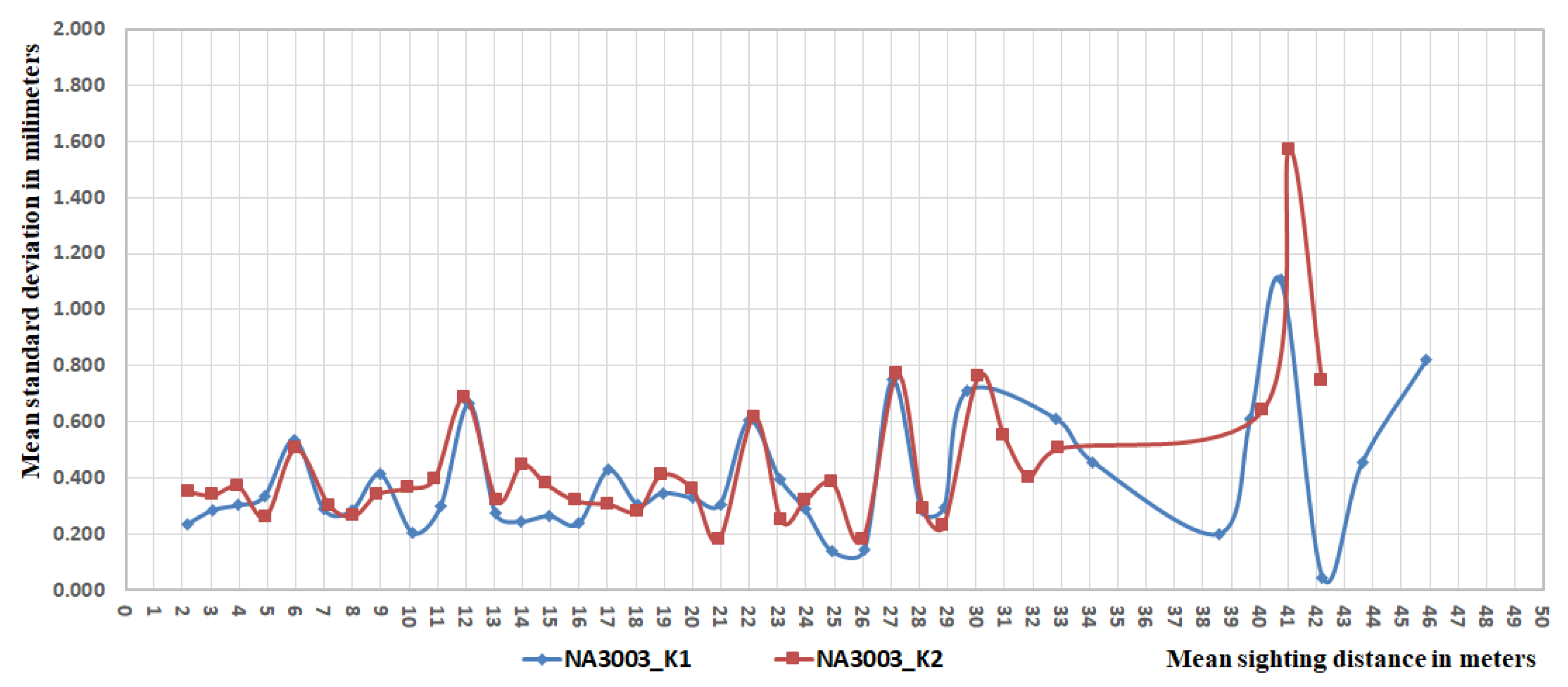
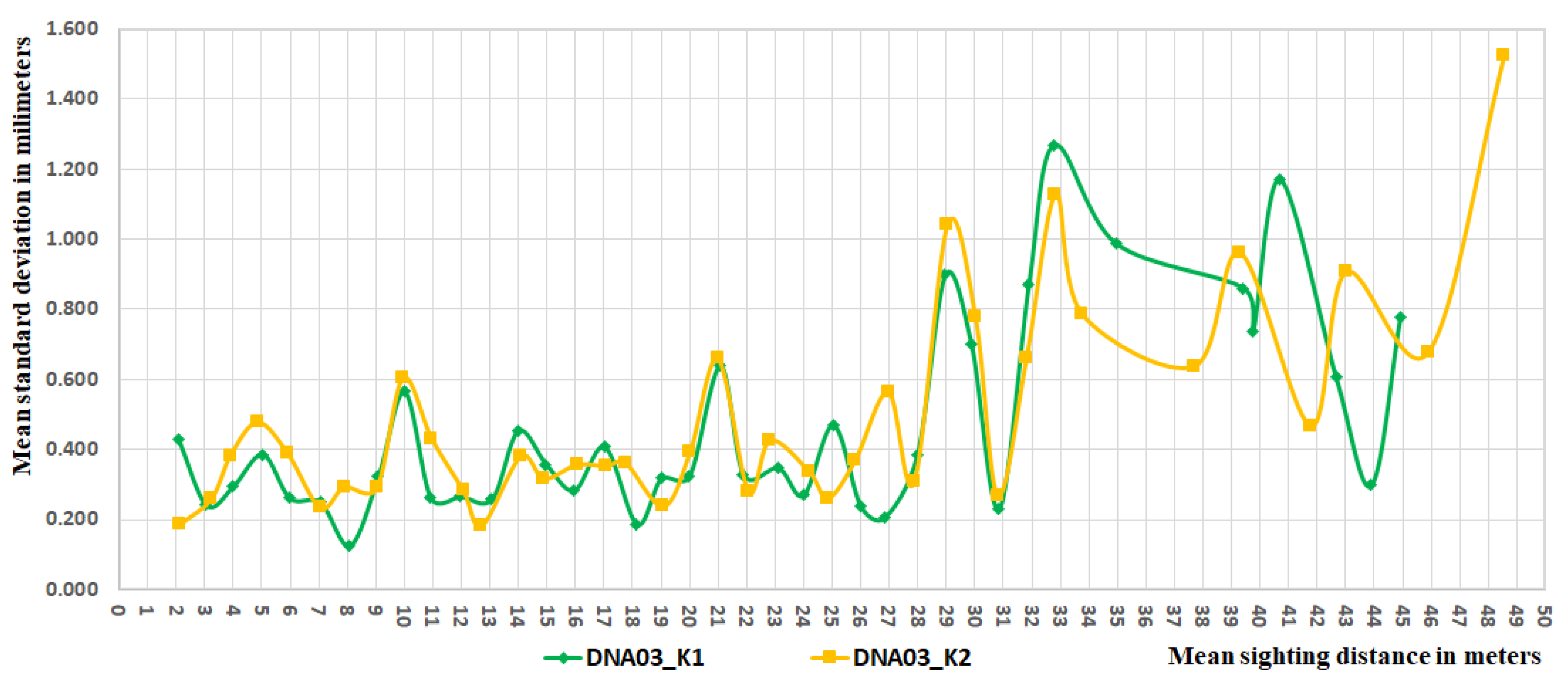
4.2. Detection of the Influence of Critical Sighting Distance

Calibrations of certain levelling devices performed on a vertical comparator are described in [1,2,8]. They have brought results concerning the scale determination, the detection of the possible errors of height deviations measured in the end sections of the staff, the determination of the influence of damaged code elements on the height readings, and the identification of the critical sighting distance of specific digital levels. The scale determination is based on using two separate runs of the levelling staff to detect and compare the edges of all code elements of the staff. The scale value of staff is then determined from a linear regression model. The second published calibration procedure is based on finding the height deviations, which rise by sighting at the end sections of levelling code staffs. It starts with defining the useable area of the staff, which varies from approximately 2.80–2.98 m to a 3 m long staff, of both Leica and Trimble systems. According to Woschitz [8], the height reading beyond the useable staff area might be wrong by more than 0.5 mm at the sighting distance of 30 m. The reason might be in an asymmetric pixel image on both ends of a staff or the refraction effect, which appears mainly by sighting the lower parts of the levelling staff. Experimental measurements at the Stanford SLAC have produced the results, published by Gassner et al. [1], which contain formulas for computing the ideal sighting section on the end of the levelling staff to avoid corrupted height differences for Leica DNA03. For the lower end, Gassner suggests the following formula:

H_lower [mm] = visible code on the staff + 20 + 7 × sighting distance [m]

(13)

and for the upper end of the levelling staff:

H_upper [mm] = visible code on the staff − 20 − 7 × sighting distance [m],

(14)

where H_lower and H_upper are the ideal sighting sections on the lower and upper ends of levelling staff equal to 10 millimetres at a sighting distance of 10 m.

Both Equations (13) and (14) are valid for sighting distances of up to 15 m. If the sighting distance is less than 3 m, the correct results are only possible in a usable area of 0.078–1.899 m using a two-meter-long levelling staff. The third published calibration procedure concerns damaged code elements’ influence on the height readings. Reference measurements realised at the TUG have brought knowledge concerning errors arising from damaged code elements, which depend on the used correlation function, which varies for the different levels. Investigation results of the critical sighting distance obtained on the SLAC vertical comparator described in [1] confirmed the assumptions of Woschitz and Brunner [6] that define the critical distance of Leica NA3000, which is 15 m. According to the obtained results, the critical distance occurs when the size of code lines projected onto the CCD array is exactly the size of one pixel or if multiple code lines are mapped to a whole number of pixels. This means that for Leica DNA03, one code element sized 2.025 mm is projected onto the CCD array with the size of one pixel at a distance of 26.7 m, and for Trimble DiNi12, the code element with a width of 20 mm corresponds to the critical distance of 10.98 m or its multiple. These described calibration outputs inspire our research based on experimental measurements to find the influence of the critical sighting distance of digital levels NA3003 and DNA03. This influence was searched by comparing height differences obtained by certain sighting distances, which were arranged into sighting groups with computed standard deviations, which represent a measure of dispersions of height differences. Standard deviations twice greater than the total standard deviation point out suspicious measurement dispersion, which indicates the existence of gross error possibly caused by critical distance influence.

Table 3. Mean standard deviations arranged into the sighting groups.

NA3003						DNA03
Locality K1			Locality K2			Locality K1			Locality K2
Sighting Distance [m]	Number of Sights	Weighted Stdev [mm]	Sighting Distance [m]	Number of Sights	Weighted Stdev [mm]	Sighting Distance [m]	Number of Sights	Weighted Stdev [mm]	Sighting Distance [m]	Number of Sights	Weighted Stdev [mm]
2.186	11	0.24	2.241	7	0.35	2.065	25	0.43	2.151	19	0.19
3.090	42	0.29	3.072	28	0.34	3.042	25	0.24	3.256	23	0.26
3.976	48	0.30	3.991	58	0.37	3.970	37	0.29	3.911	40	0.38
4.901	32	0.34	4.942	23	0.26	5.014	34	0.39	4.863	47	0.48
5.962	16	0.54	6.000	22	0.50	5.966	33	0.26	5.920	17	0.39
6.990	24	0.29	7.193	19	0.30	7.046	20	0.25	7.062	49	0.23
7.980	56	0.28	8.058	50	0.27	8.073	23	0.13	7.907	24	0.29
8.994	24	0.41	8.890	22	0.34	9.071	15	0.32	9.044	29	0.29
10.130	8	0.21	9.986	8	0.36	9.990	22	0.56	9.956	16	0.60
11.109	14	0.30	10.901	30	0.40	10.910	23	0.26	10.964	13	0.43
12.121	12	0.67	11.983	12	0.69	11.953	21	0.27	12.078	27	0.28
13.048	40	0.27	13.105	47	0.32	13.059	25	0.26	12.720	13	0.18
13.925	45	0.25	13.987	39	0.45	13.978	17	0.45	14.082	43	0.38
14.948	15	0.27	14.843	10	0.38	14.960	24	0.36	14.907	28	0.32
15.983	9	0.24	15.889	22	0.32	15.940	39	0.28	16.059	11	0.36
17.032	28	0.43	17.048	15	0.31	17.013	18	0.41	17.092	50	0.35
18.057	48	0.31	18.082	59	0.28	18.141	27	0.19	17.761	21	0.36
18.942	35	0.35	18.903	22	0.41	18.999	19	0.32	19.086	31	0.24
20.018	4	0.33	20.010	19	0.36	19.988	27	0.32	20.024	30	0.39
20.974	16	0.31	20.932	13	0.18	21.061	24	0.64	20.995	9	0.66
21.991	18	0.61	22.182	13	0.62	21.879	13	0.33	22.063	23	0.28
23.077	32	0.40	23.139	32	0.25	23.098	20	0.35	22.825	18	0.43
23.965	51	0.29	23.964	43	0.32	23.986	16	0.27	24.197	25	0.34
24.922	10	0.14	24.938	10	0.38	25.024	20	0.47	24.857	39	0.26
26.062	8	0.14	25.996	8	0.18	25.984	27	0.24	25.808	13	0.37
27.041	21	0.75	27.228	7	0.77	26.821	11	0.21	26.971	15	0.56
28.081	19	0.28	28.134	28	0.29	27.972	22	0.38	27.877	38	0.31
28.877	23	0.30	28.851	21	0.23	28.956	9	0.90	29.051	2	1.04
29.678	5	0.71	30.100	4	0.76	29.867	15	0.70	30.021	5	0.78
32.833	3	0.61	31.001	11	0.55	30.835	12	0.23	30.805	8	0.27
34.124	9	0.46	31.895	6	0.40	31.939	6	0.99	31.811	2	0.66
Total standard deviation		0.31	Total standard deviation		0.37	Total standard deviation		0.35	Total standard deviation		0.38

shows the measured height differences arranged into sighting groups and the appropriate standard deviations that point to their dispersion in the frame of a sighting group. The total value of standard deviation was computed in the reference system separately for each digital level and each experimental locality and is displayed at the end of Table 3. The mean standard deviations are graphically displayed separately for the levelling device Leica NA3003 in Figure 1 and for the DNA03 in Figure 2.

5. Discussion

The first part of the paper aimed to verify the dependence of the accuracy of measured height differences on the sighting distance. The measurement and processing methodology of digital levelling was based on the assumption of eliminating the subjective effects on the measurement accuracy and appearance of the new kinds of instrumental errors resulting from their digital technology as was mentioned in [23]. This means that the ratio between random and systematic influence should change. The current levelling accuracy characteristics are based on the cumulation of partial random and systematic effects on a station, and therefore the experimental measurements consisted of verifying the representation of elementary errors, divided into four groups according to their dependence on sighting distance [14]. The main aim of the paper was to detect the influence of critical sighting distance of specific digital levels on measured height differences and compare it with the results found by Gassner, Ruland and Dix in [1,2] via calibration on a vertical comparator. The experiment was based on measuring height differences in fixed points from different sighting distances with digital levels of Leica NA3000 and Leica DNA03. For this purpose, the standard deviations were calculated in each sighting group created around the average sighting distance and were compared with the total standard deviation that represents tolerance. The double-increased standard deviation that appeared in the same sighting group in independent observational localities K1 and K2 can show the probable influence of critical sighting distance.

The results in Table 3 and Figure 1 and Figure 2 show the increased standard deviations for Leica NA3003 around the sighting distances 12 m, 22 m, 27 m and 30 m. Twice higher standard deviations of the Leica DNA03 level were observed at distances of 21 m, 29, 30 m and 32 m while the values with sighting distances over 35 m were not involved in the analysis because of the increased dispersion of measured values (see Figure 1 and Figure 2). The sighting distances with increased values of standard deviations of both digital levels do not correspond to the critical ones published by Gassner and colleagues [1,2]. However, the experimental results require further investigation. The uncertainties corresponding to detected sighting distances either showed a different systematic source, critical sighting distance varies from instrument to instrument or it is necessary to revise the research methodology. The second part of the experiment consisted of an estimation of particular errors on a station represented by error model arguments to find the ratio between dependent and independent errors on a sighting distance. Though the representation of the levelling errors varied from station to station, the common characteristic in their numerical order can be found in the whole levelling route in both experimental localities. The results from the estimation of the mathematical model that is published in Table 1 and were validated by an analysis of variances show that digital level NA3003 has approximately 49.9% levelling errors that are independent of the sighting distance and DNA03 has approximately 65% dependent errors dependent on the sighting distance. Estimations in Table 1 confirm the well-known expectations, which are also presented in [14], that error arguments c and d have insignificant importance.

6. Conclusions

The calibration tests of digital levels Leica NA3003 and DNA03 published by researchers Gassner [1,2] introduced the concrete values of critical sighting distances, which caused the increased occurrence of levelling errors when the size of code lines responds to the size of one pixel of the CCD camera or its multiple. The described experiment, which consisted of many intermediate sights measured in two independent levelling routes, did not confirm the influence of a critical distance of 15 m for level NA3003 and 26.7 m for level DNA03 on the precision of measured height differences. However, digital levels showed systematic influences at other sighting distances: 12 m, 22 m, 27 m and 30 m for NA3003 and 21 m, 29 m, 30 m and 32 m for DNA03. The results did not correspond to the multiple code sizes of both digital levels. The reason may be the influence of another systematic error that is assumed to be verified by an independent methodology in future. When analysing the results, it is necessary to take into account that they are compared with findings obtained under significantly more accurate laboratory conditions using highly accurate and specialized calibration equipment. Even if there is an influence of the critical sighting distance on digital levelling, it may not have been detected by the proposed methodology, based on the detection of measurement uncertainty that often appears with an increased value of the standard deviation. In the future, it might be useful to compare results from precise digital and analogue levels in places where the influence of critical sighting distance is expected or to compare precise digital devices of different manufacturers. The analysis of elementary error propagation on a station leads to finding the ratio between errors dependent on and independent of the sighting distance through parameter estimation in the mathematical “error” model. The variances (6) computed from the estimates of error parameters displayed in Table 1 show that digital level NA3003 has approximately 50% of levelling errors that are dependent on the sighting distance and DNA03 has approximately 35%. Because of the precise levelling method, the accuracy analysis concerned only height differences, which do not exceed a sighting distance of 35 m. Results above this limited sighting distance detected much more increased dispersions.

Since the research aimed to compare the results of laboratory tests of specific level-ling devices, obtained by the authors in [1,2], which are naturally much more accurate than field measurements, the methodology of the measurements analysis was based on the assumption that the dispersions of height differences obtained at the critical sighting distance increase much more. The research output pointed to the occurrence of levelling errors in places that do not match the assumptions. Therefore, the task of future experiments will be to compare the results of several digital levelling systems and to focus the methodology of measurement analysis on the evaluation of the height differences found in these suspicious measurement places. The estimation process of finding the proportion of levelling errors depending on the sighting distance has produced an interesting result. The unknown estimations of the mathematical model showed that DNA03 has a larger proportion of errors depending on the sighting distance (65%) than the older instrument NA3003 (50%).

References

1. Gassner, G.L.; Ruland, R.; Dix, B. Investigations of digital levels at the SLAC vertical comparator. In Proceedings of the 8th International Workshop on Accelerator Alignment (IWAA2004), CERN, Geneva, Switzerland, 4–7 October 2004. [Google Scholar]
2. Gassner, G.L.; Ruland, R.E. Investigations of Levelling Equipment for High Precision Measurements; SLAC, Stanford University: Menlo Park, CA, USA, 2005; pp. 1–8. Available online: https://www.slac.stanford.edu/pubs/slacpubs/12250/slac-pub-12326.pdf (accessed on 18 May 2024).
3. Baričevič, S.; Satroveški, T.; Barkovič, D.; Zrinjsti, M. Measuring Uncertainty Analysis of the New Leveling Staff Calibration System. Sensors 2023, 23, 6358. [Google Scholar] [CrossRef] [PubMed]
4. Kuchmister, J.; Gołuch, P.; Ćmielewski, K.; Rzepka, J.; Budzyń, G. A functional-precision analysis of the Vertical Comparator for the Calibration of geodetic Levelling Systems. Measurement 2020, 163, 107951. [Google Scholar] [CrossRef]
5. Takalo, M.; Rouhiainen, P. On System Calibration of Digital Level. In Proceedings of the 14th International Conference on Engineering Surveying, Zürich, Switzerland, 15–19 March 2004; p. 10. [Google Scholar]
6. Woschitz, H.F.K.; Brunner, F.K. Development of a Vertical Comparator for System Calibration of Digital Levels. Osterr. Z. Vermess. Geoinf. 2003, 91, 68–76. [Google Scholar]
7. Woschitz, H.; Brunner, F.; Heister, H. Scale Determination of Digital Levelling Systems using a Vertical Comparator. In Fachbeiträge; Graz University of Technology and Bundeswehr University Munich, FIG XXII International Congress: Washington, DC, USA, 2002; zfv 1/2003; pp. 1–13 (2003). [Google Scholar]
8. Woschitz, H.; Brunner, F.K. System Calibration of Digital Levels—Experimental Results of Systematic Effects; Graz University of Technology: Graz, Austria; pp. 1–8. Available online: https://www.tugraz.at/fileadmin/user_upload/Institute/IGMS/laboratory/diglevelcal/2002_WHD_FKB_ingeo_reprint.pdf (accessed on 18 May 2024).
9. Rekus, D.; Aksamitauskas, V.C.; Giniotis, V. Application of Digital Automatic Levels and Impact of their Accuracy on Construction Measurements. In Proceedings of the 25th International Symposium ISARC, Vilnius, Lithuania, 26–29 June 2008; pp. 625–631. [Google Scholar]
10. Sjöberg, L. An Analysis of Systematic and Random Errors in the Swedish Motorized Levelling Technique; Lantmäteriet, National Land Survey: Gävle, Sweden, 1981; 25p, Available online: https://www.lantmateriet.se/globalassets/geodata/gps-och-geodetisk-matning/rapporter/1981-2.pdf (accessed on 18 May 2024).
11. Yaprak, S. Accuracy of a Second-Order First-Class Precise Levelling Project, Bollettino di Geofisica Teorica ed Applicata, Vl. 60; Department of Geomatics, Gaziosmanpas a University: Tokat, Turkey, 2019; pp. 39–48. [Google Scholar]
12. Zilkovski, D.B. A Priori Estimates of Standard Errors of Levelling Data; National Geodetic Survey: Silver Spring, MD, USA, 1991; 12p, (Nationa Geodetic Survey June 2018). Available online: https://www.ngs.noaa.gov/wp-content/uploads/2018/06/Zilkoski1991-2.pdf (accessed on 19 June 2023).
13. Errors in Levelling: Types and Their Correction. Different Types of Errors Encountered in Surveying Operations. Available online: https://testbook.com (accessed on 19 June 2023).
14. Böhm, J.; Svoboda, J. Geometrická Nivelase; SNTL: Praha, Czechoslovak Republic, 1960; 288p. [Google Scholar]
15. Craymer, M.R. Data Series Analysis and Systematic Effects in Levelling. Master’s Thesis, Department of Civil Engineering University Toronto, Toronto, ON, Canada, 1984; p. 126. Available online: https://gge.ext.unb.ca/Research/GRL/LSSA/Literature/Craymer1984.pdf (accessed on 5 May 2018).
16. Craymer, M.R.; Vaníček, P. Further analysis of the 1981 Southern California field test for levelling refraction. J. Geophys. Res. 1986, 91, 9045–9055. [Google Scholar] [CrossRef]
17. Saaranen, V. Robotization of Precise Levelling Measurements. Available online: https://mycoordinates.org/robotization-of-precise-levelling-measurements/ (accessed on 5 May 2018).
18. Cvetkov, V. Two Adjustments of the Second Levelling of Finland by Using Nonconventional Weights. Available online: https://www.degruyter.com/document/doi/10.1515/jogs-2022-0148/html (accessed on 14 March 2023).
19. Elhassan, I. Comparison of indoor and outdoor Accuracy Performance of Optical Automatic, Digital and Laser Levels. IJERT 2022, 11, 6. Available online: https://www.ijert.org/comparison-of-indoor-and-outdoor-accuracy-performance-of-optical-automatic-digital-and-laser-levels (accessed on 14 November 2022).
20. Vignal, J. Evaluation de la Précision d’une Méthode de Nivellement; Bulletin Géodesique: Paris, France, 1936; pp. 1–159. [Google Scholar]
21. Bomford, G. Geodesy, 3rd ed.; Clarendon Press: Oxford, UK, 1971; 731p. [Google Scholar]
22. Ingesand, H. Check of Digital Levels. FIG XXII International Congress, TS5.11 Standards, Quality Assurance and Calibration, Washington, DC, USA. 2002, p. 10. Available online: https://www.fig.net/resources/proceedings/fig_proceedings/fig_2002/Ts5-11/TS5_11_ingensand.pdf (accessed on 14 March 2023).
23. Ingensand, H. The Evolution of Digital Levelling Techniques—Limitations and New Solutions; FIG Report Activities, Comm 5; FIG Report: Zürich, Switzerland, 1999. [Google Scholar]
24. Clarke, B.R. Linear Models: The Theory and Application of Analysis of Variance; Wiley: Hoboken, NJ, USA; Toronto, ON, Canada, 2008; 241p, ISBN 978-0-470-02566-6. [Google Scholar]
25. Koch, K.R. Introduction to Bayesian Statistics, 2nd ed.; Springer: Berlin/Heidelberg, Germany, 2007; 249p, ISBN 978-3-540-72723-1. [Google Scholar]
26. Niemeier, W. Ausgleichungs-Rechnung; Walter de Gruyter: Berlin, Germany; NewYork, NY, USA, 2002; 407p, ISBN 3-11-014080-2. [Google Scholar]
27. Cochran Variance Outlier Test. Available online: https://www.itl.nist.gov/div898/software/dataplot/refman1/auxillar/cochvari.htm (accessed on 12 November 2023).
Figure 1. The dependence of the levelling accuracy on the mean sighting distance of the level Leica NA3003.
Computation 12 00111 g001
Figure 2. The dependence of levelling accuracy on the mean sighting distance of the level Leica DNA03.
Computation 12 00111 g002