Abstract
The article discusses the application of quaternion Fourier transforms and quaternion algebra to transform Maxwell’s equations. This makes it possible to present the problem of magnetotelluric sensing (MTS) in a more convenient form for research. Studies of the inverse MTS problem for multi-layer regions are presented using the differential evolution method, which demonstrates high convergence. For single-layer regions, a new method for solving inverse problems based on minimizing the quadratic functional using conjugate optimization methods is considered. Numerical results obtained using special Python libraries are presented, with analysis and conclusions.
1. Introduction
Currently, magnetotelluric sounding (MTS) is a powerful and relevant tool for the study of underground geology and a variety of geophysical phenomena. The application of this method provides valuable information about the composition and structure of the Earth, which is important for solving a variety of applied and scientific problems. The natural electromagnetic field contains fluctuations of various frequencies. As a result of a phenomenon known as the skin effect, the higher-frequency vibrations of the MT field weaken faster with increasing depth, whereas the low-frequency components of the spectrum penetrate to greater depths. Consequently, the high-frequency components of the field contain information, mainly about the surface layers of the section. With decreasing frequency, the contribution of deeper parts of the section to the observed field increases, which allows us to obtain information about the deep parts of the geoelectric section [1,2,3]. The MTS method has a number of advantages. Unlike other methods, the use of generator sets is not required, however, it allows research to be carried out to a considerable depth and is available only for studies using methods with a controlled source.
The theoretical foundations of the MTS method are based on the Maxwell equation systems, which describe the electromagnetic field. Maxwell’s equations are the basis of classical electrodynamics and describe the interaction of electric and magnetic fields, as well as the propagation of electromagnetic waves in space [1].
In recent years, scientists have been increasingly interested in using quaternion Fourier transforms (QFTs) to solve partial differential equations. In [4,5], the basic properties of direct and inverse partial differential transformations using QFT were studied and proved, and the applications of QFT for solving problems of thermal conductivity and the wave equation were considered. It is shown that the use of the QFT makes it possible to exclude one of the spatial or temporal variables. After the transformation, the problem is considered in a private domain, allowing us to preserve the physical nature of the equation itself. New scientific results have also been obtained to improve the modification of QFT and prove its unique properties, such as convolution and correlation.
Since Hamilton’s work, quaternions as a mathematical tool have been used to formulate Maxwell’s equations in the theory of electromagnetism. Applying quaternions to Maxwell’s equations brings them to a convenient form.
In [6,7], the use of quaternions allowed the author to present electromagnetic fields in a compact form and write down a fundamental solution.
In many works [8,9,10], the properties of integration and differentiation of quaternion functions have been proved, and tables convenient for use have been compiled. The application of QFT simplifies the system of Maxwell’s equations while preserving the spectral properties of impulses in space.
The general formulation of the MTS inverse problems is to restore the distribution of the physical parameters of the environment in the Earth’s crust according to the data of physical fields measured on the Earth’s surface. The main purpose of this approach is to study the structure of the near-surface layer of the Earth’s crust, as well as to search for mineral deposits. The inverse MTS problem makes it possible to determine a geophysical model (resistance) based on measurements of apparent resistance. Since the early 1950s, when the MTS method was proposed, methods for solving inverse problems in this area began to develop and find applications in various fields, including marine geophysics, environmental studies, analysis of the electrical structure of the earth’s crust and upper mantle, geological research, and exploration of mineral deposits [11,12].
MTS inverse problems are often characterized by incorrectness, which usually leads to low quality solutions and high sensitivity to noise in the input data. The standard way to deal with these problems is to reformulate the task. Inverse problems in this field are usually nonlinear and non-unique [13,14,15,16]. To solve them, geophysicists usually use linearized regularization methods [17,18]. In the works [2,3,13], multi-layer models for the numerical solution of the coefficient inverse problem of MTS are considered.
When using machine learning methods, this paradigm can be changed by adding additional information. This information can either be entered directly into the algorithm, or used indirectly by taking it into account when forming a training sample. An approach based on the indirect use of additional information, based on alternative measurement methods or structural assumptions, is shown in [19]. The method, which includes the direct introduction of additional information, is considered in the work [20,21,22,23]. This method is associated with the integration of geophysical methods, which involves the simultaneous use of data from several geophysical methods to solve the inverse problem.
Among the widely used methods of inverse MTS problems, the following can be distinguished: the Occam inversion method, which builds a model with minimal roughness at a given degree of discrepancy, providing a stable and rapidly converging solution [24,25]; fast relaxation inversion, where horizontal derivatives are approximated based on the fields of previous iterations [26]; and nonlinear conjugate gradients that prevent the need to evaluate the complete Jacobi matrix and solve the linearized inverse problem at each iteration step [18]. These methods of inverse problems, as a rule, modify the objective functional to reduce the uniqueness of the solution.
In this study, multi-layer and single-layer models are considered for determining the resistance and power of horizontal isotropic layers in the problem of MTS. For the first time, the use of quaternion Fourier transforms for solving stationary and non-stationary MTS problems described by Maxwell’s equations is investigated. The application of quaternions to Maxwell’s equations leads them to a convenient form for solving. Algorithms for the numerical solution of the considered models have been developed. In the proposed approaches for solving inverse problems, quadratic functionals are minimized. An adaptive algorithm of differential evolution has been developed for the multi-layer model. Numerous calculations of the single-layer and multi-layer MTS problem in complex variables using special Python libraries are presented. The numerical results are analyzed and the revealed patterns are presented in the form of graphs.
2. Materials and Methods
This study used simulations of the variation of the Earth’s electric field. Magnetic variations and electric earth currents observed on the Earth’s surface follow specific relationships, as they represent different manifestations of the Earth’s natural electromagnetic field [27]. This article examines the theoretical relationship between magnetic variations and the Earth’s currents from the point of view of Maxwell’s equations. The studied theoretical issues allow numerical modeling of the electrical properties of the deep layers of the Earth’s crust.
The study assumes consideration of lithospheric layers consisting of an upper conductive layer (sedimentary cover), intermediate resistive layers (consolidated crust and upper mantle), and a conductive base (asthenosphere) [1].
To solve this problem, boundary conditions of the third kind are considered, since they generalize the properties of Dirichlet and Neumann conditions. When solving the problem with the presented boundary conditions, it is assumed that the medium of a single-layer region is homogeneous and isotropic. For multi-layered regions or areas with more complex geometries, other boundary conditions may be required that take into account transitions between layers and their interaction.
2.1. Transformation of Maxwell’s Electromagnetic Field Equations
Consider the system of Maxwell’s equations in differential form
where is the electric field vector, unit [V/m], is the vector of the magnetic field, unit [A/m], is the vector of electric induction, unit [C/m2], is the vector of magnetic induction, unit [Wb/m2 = T], is the vector of density of electric current, unit [A/m2], , -conductivity current density, and is the density of external currents. is the volume density of the external electric charge, [].
It is well known that Equation (1) describes the law of total current; Equation (2) describes Faraday’s law of electromagnetic induction, the third equation follows on from Gauss’s law, and the fourth equation means that the flux of magnetic charges does not exist.
In the system (1)–(4), if considered coordinate-wise, then the number of equations is (8) and the number of scalar unknowns is 15. Therefore, material equations of the following form are introduced:
where F/m, Gn/m, , is the remote electrical conductivity of the medium, with the unit of measurement .
This introduced the notation , . Substituting (5)–(7) into (1)–(4), there will be 8 scalar equations for 6 scalar unknowns of the function
where is the density of external currents, is the volume charge density, and is the conductivity current density.
If the operator is from both sides of Equation (9), then it turns out
According to the rules of vector analysis, the following takes place:
where from Equation (10). From (12), taking into account (10) and (13), the following was obtained
Similarly, a hyperbolic equation for was obtained
Equations (14) and (15) for and are of hyperbolic type and differ only in the right hand side. Therefore, in general, it can be written as
If is represented as a harmonic process
Substituting in (16), the Helmholtz equation was obtained
where is complex dielectric constant.
Equations (14) and (16) are reduced to an equation of the form (18) using the method of complex amplitudes or direct Fourier transform. This approach is widely used to solve applied problems.
2.2. Application of QFT for a Non-Stationary Problem
Further, using QFT, Cauchy problems for hyperbolic-type equations are obtained. As indicated in Section 2.1, the system of Maxwell’s equations is solved by methods of complex amplitudes and direct Fourier transform. The use of QFT makes it possible to obtain a linear differential equation of the second order, the right side of which contains the spectra of pulses.
The QFT is an innovative tool in the field of signal and image processing, enriching the arsenal of data analysis and processing methods. They are a generalization of the classical Fourier transform, which is used for signal and image processing, including three-dimensional and four-dimensional samples.
Physical signals often have a three-dimensional nature, reflecting the three-dimensional space of the environment. This highlights the need to use three-dimensional samples in the analysis of such signals. It is worth noting separately that color images, in turn, consist of three components per pixel, which is due to the trichromatic nature of human vision. In this regard, QFTs are proving to be very effective tools for processing such complex data.
It is important to note that the fourth dimension of quaternions plays an essential role, allowing the representation of signals in the frequency domain using four dimensions. This not only expands the possibilities of data analysis and processing, but also allows the use of homogeneous coordinates to represent the most general set of geometric operations in three dimensions.
QFTs play a key role in translating a signal or image from the temporal or spatial domain to the frequency domain. Thanks to this representation, we can analyze signals and images in the frequency domain, which can lead to fast and efficient information extraction.
QFTs are reversible, which means that the original signals or images can be reconstructed from their representation in the frequency domain. Moreover, this representation can be modified before inverting the transformation, which opens up possibilities for modifying signals or images, for example, suppressing, attenuating, or amplifying certain frequency components.
The QFT is also a powerful tool for analyzing and processing signals and images. Their application opens up new perspectives for working with three-dimensional and four-dimensional data, enriching our knowledge and methods in the field of digital signal and image processing.
Consider the following problem:
To solve the problem (19)–(21), the theory of quaternions and quaternion Fourier transforms was applied. The quaternion algebra over , denoted as , is an associative non-commutative four-dimensional (4D) algebra,
where are imaginary units that follow the multiplication rules established by Hamilton:
In [8], the following definition of QFT is given:
Definition.
Let . The QFT transformation for f is a function of , which is defined by the following formula:
are frequencies according to spatial variables
Using the tabular formulas of the QFT, transformation of the operator from [9], and the multiplication rules (23) for Equation (19), the following was obtained:
Suppose that
Introducing the notation , Equation (23) was rewritten in the following form:
where .
The general solution (26) is represented as
First, consider the following characteristic equation for a homogeneous equation:
the solution of which has the form
where
Given the right side of Equation (26) and the initial conditions, the solution is represented as
The application of the inverse QFT transformation allows us to write the solution of the problem (19)–(20) in the form
2.3. Application of QFT for a Stationary Problem
The application of QFT is not limited to spatial variables only, but can also be extended to a temporal variable. The use of QFT in time translates the original problem into the frequency domain, which allows for a more in-depth investigation of its nature.
The key advantage of using QFT in the time domain is the ability to analyze the frequency characteristics of a signal or image. In the frequency domain, it becomes more understandable to identify the main components of the signal and their interactions. This allows in-depth study of spectral features and variations of electromagnetic fields, which can be important in solving problems of mathematical geophysics.
Consider the following boundary value problem in the domain:
The right-sided QFT transformation used for the problem (26)–(30) has the following form:
where , is a pure unit quaternion for which the following equality holds:
Using the QFT transformation for Equation (26)
Hence, assuming that the electromagnetic field is homogeneous in the and directions, the following one-dimensional problem for the Helmholtz equation with quaternionic variables was obtained:
To obtain a solution to the original problem, the inverse QFT transformation is used, which is defined as
The solution of the problem (34)–(36) in quaternion variables strongly depends on the sign of the discriminant of the characteristic equation [28,29]. Therefore, the numerical solution of MTS problems is further carried out in complex variables. The authors set a goal to present a more simplified solution methodology. The proposed solution technique can be generalized to quaternionic variables, since Python has an extension to quaternionic numbers.
The QFT can process vector data more stably because quaternions naturally include information about the rotation and orientation of vectors. Combining operations into a single expression can reduce the number of intermediate calculations, which reduces the accumulation of rounding errors.
3. Results and Discussion
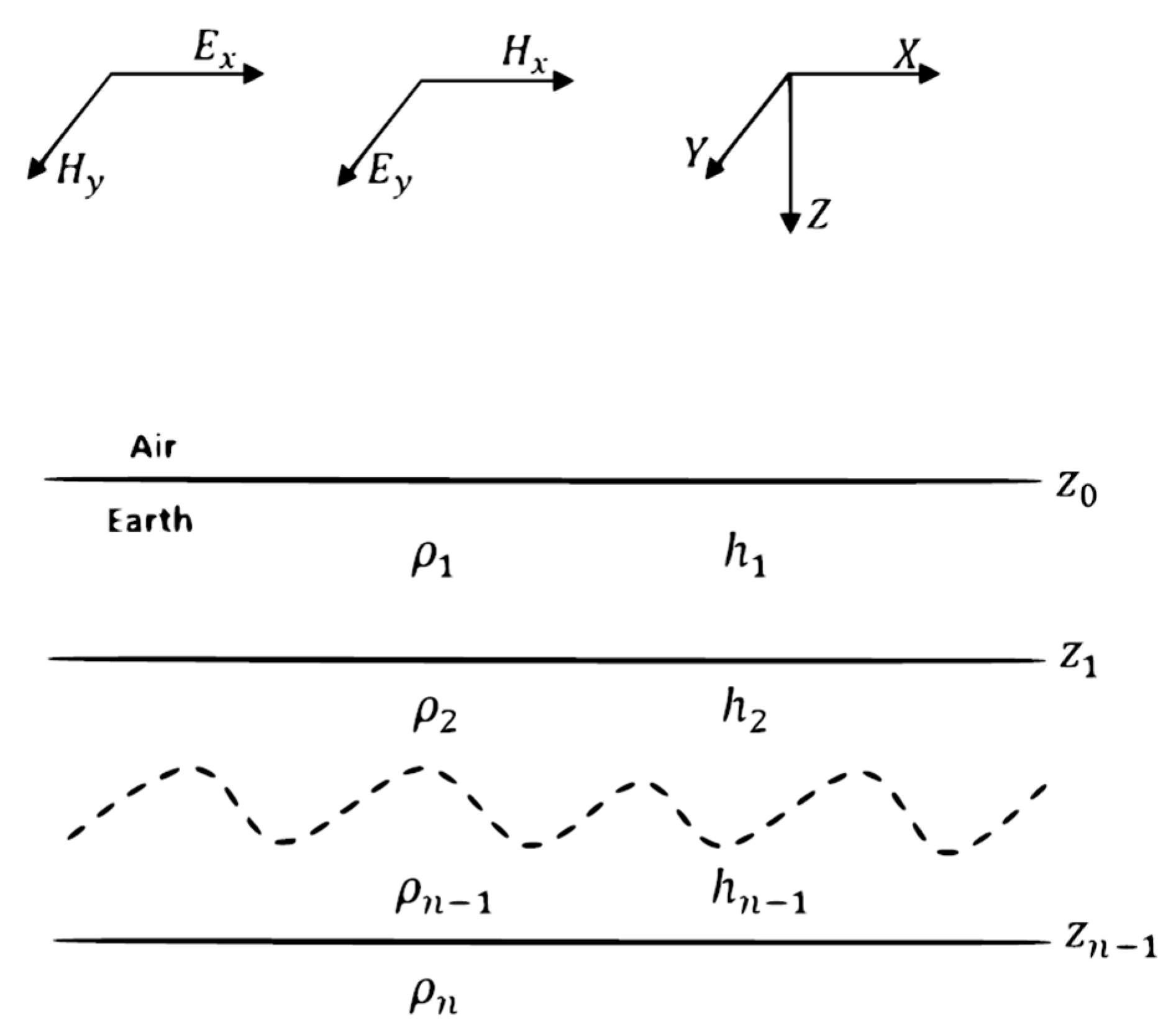
With regard to the formulation of the problem of magnetotelluric sensing, in this section, there will be a considered schematic representation of the model section (Figure 1). The model consists of several horizontally homogeneous and isotropic layers with different properties, resistivity and power (where is the layer number).

Figure 1.
Geoelectric model of a horizontally layered medium used in MTS.
Consider a right-hand coordinate system, where the axis is pointing downwards, and the and axes are located in the plane separating air and Earth (Figure 1). The earth is divided into n horizontal isotropic layers with resistances and capacities . The power of the last layer (the th layer) is considered infinite. The upper half-space () is filled with non-conducting air with a permittivity of . The magnetic permeability is constant and equal to one in all areas of the model [8,19].
Suppose that a primary elliptically polarized plane homogeneous monoharmonic electromagnetic wave , falling from above onto the Earth’s surface, propagates along the axis. This wave can be decomposed into two independent linearly polarized plane homogeneous waves, the wave and wave. Wave causes the ground electric field and the magnetic field . Wave causes the electric field , and the magnetic field . By superposition of these elementary waves, a field was obtained:
complex vectors , which are always orthogonal. Indeed, it follows from the conditions of axial symmetry of the medium that
whence,
The value
is called impedance. On the Earth’s surface, at , the input impedance was obtained, where the n index corresponds to the number of layers in the section.
Determination of the Input Impedance Using the Recurrent Formula
According to Formula (39), it is sufficient to consider the components and . In each layer, the value satisfies the one-dimensional Helmholtz equation:
where is the wave number for the th layer, defined in such a way that :
where is the resistivity of the th layer, respectively, is the frequency.
The general solution of the considering equation has the form:
where and are constants depending on the cut parameters and frequency. The exponent is a set of plane homogeneous waves propagating from top to bottom, and the exponent is a set of plane homogeneous waves propagating from bottom to top. For the nth layer (the underlying base), the value of is zero, which follows from the condition of attenuation of the electromagnetic field at .
To determine the component, our study uses the formula derived from the second Maxwell equation. From Maxwell’s second equation, the following expression will be obtained:
According to (39), (41), and (42), the impedance at the level within the layer can be expressed as follows:
By applying the identities of N.V. Lipskaya [30], we obtain a recurrent formula that expresses the dependence of the impedance on the roof of the -th layer on the impedance on the -th layer , the properties of the layer ( and ), and the frequency . It allows us to express the impedance on the roof of the -th layer through the specified parameters.
The impedance on the surface of the lower (th) layer is equal to:
This condition follows from the law of conservation of energy and electromagnetic induction. If the tangential components of the field were not continuous, then there would be sharp changes in the electric and magnetic fields at the interface, which would lead to a violation of energy conservation and electromagnetic induction.
Using the impedance at the lower boundary of the (st) layer, its value at the previous (nd) boundary will be calculated. Then at the next (rd) boundary, and so on, until the Earth’s surface will be calculated. The value of the impedance on the Earth’s surface will depend only on the properties of the layers (resistances and powers) and frequency. This value is a solution to the direct MTS problem in the Tikhonov–Cagniard model.
For the convenience of programming, we will bring these formulas to a certain form. The impedance on the roof of the -th layer can be presented in the following form [3]:
here is the reduced impedance, depending on the properties of the medium:
where . At relatively high frequencies, the function depends mainly on the properties of the upper layers of the section, and at low frequencies, on the properties of deep layers. Therefore, the function can be called the frequency response of a horizontally layered section.
One of the main characteristics in the study of a horizontally layered medium is the apparent resistance, which is denoted as . In the formulation of the direct problem, it is required to find the function . The formula used to sequentially recalculate the reduced impedance from the lower boundary (where ) to the Earth’s surface can be written as follows in the form of recalculation of into :
Expressing the hyperbolic arctangent in terms of the natural logarithm and using the following notation:
the final formula for calculating the reduced impedance will be obtained:
Using the resulting formula, a program can be created to solve a direct problem in the one-dimensional case. Based on this fractional–linear ratio, an algorithm has been developed to calculate the apparent resistance of a horizontally layered medium.
4. Numerical Results of Solving the Direct and Inverse MTS Problem
The model problem under consideration includes three layers, each of which is characterized by the values of resistivity and power (where m = 1, 2, 3 is the layer number) [31]. In each of these layers, the magnetic permeability is equal to 1. In this model, the Earth’s crust is divided into horizontal isotropic layers, each of which has its own values of resistivity and power . It is assumed that the power of the last layer (the third layer) is infinite.
During exploratory studies, fluctuations in the magnetic telluric field are recorded, having a period from fractions of a second to several minutes, known as short-period oscillations (SPO). Short-period oscillations occur under the influence of charged particles emitted by the sun entering near-Earth space. To visually represent the graph of apparent resistance on the time axis, is often used, which allows you to obtain information about the characteristics of the geoelectric section.
The relationship between frequency and period is determined in accordance with [1]:
For numerical calculation, certain period values were selected, which were determined based on the physical considerations described in [1].
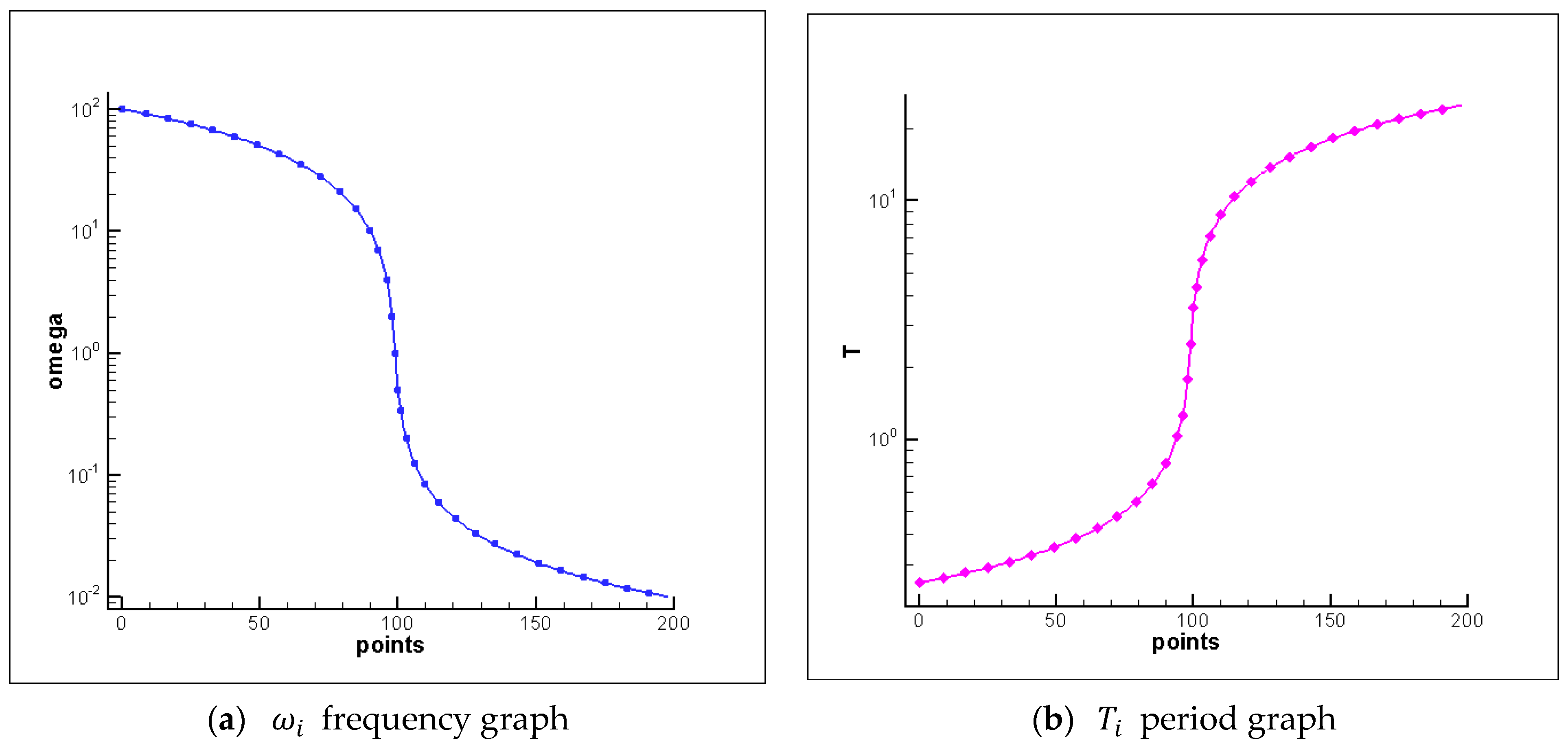
For calculations, the frequency values in the repartitions of were considered. As can be seen from Figure 2a, the values of are defined for 200 points and are inversely proportional to the values of the period (Figure 2b).
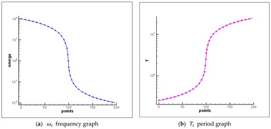
Figure 2.
Frequency (a) and period (b) graphs for the points taken for the computational experiment.
In the direct problem, it is necessary to calculate the function , which represents the apparent resistance, using the Formula (38). The reduced impedance is determined as follows:
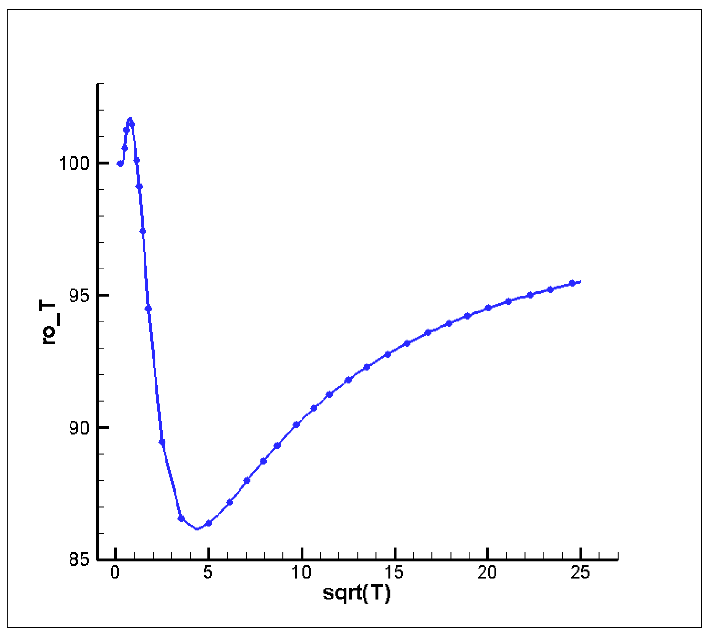
Figure 3 shows a graph of the apparent resistance for this medium model.
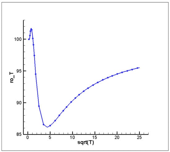
Figure 3.
Graph of apparent resistance.
The apparent resistance graph demonstrates the correspondence of the reduced curve with theoretical concepts of apparent resistance. It is noticeable that at high frequencies (small periods), the apparent resistance function depends on the upper layer, and as the period increases, we get information about the second and third layers.
4.1. Mathematical Formulation of the Inverse MTS Problem
The inverse MTS problem involves a function of many variables, where some variables are fixed, such as the number of layers and the frequency of the incident wave, while other variables vary, such as the thickness of the layers and their resistivity. The purpose of the inverse problem is to find the values of layer power and resistivity that minimize the sum of the squares of the deviations between the theoretical values of the apparent resistance modulus and the measured values for a given set of frequencies.
Mathematically, the problem is formulated as follows [3]:
where , .
4.2. The Method of Differential Evolution
In the field of scientific and engineering research, global minimization of target functionality is one of the key tasks. The main goal is to find the optimal values of system parameters to optimize certain system properties. Usually, the system parameters are represented as a vector. The objective function is a criterion that we strive to minimize in order to achieve an optimal solution.
There are many methods of global minimization, each of which has its advantages and limitations. Some of the most common methods include evolutionary algorithms, genetic algorithms, particle swarm methods, annealing simulation optimization methods, and more [32,33,34,35]. And when the objective function is nonlinear and undifferentiable, direct search methods are preferred. The most well known of these methods are the Nelder Mead algorithms, the Hooke–Jeeves method, genetic algorithms (GAs), and evolutionary strategies (ESs). These methods are effective in solving optimization problems with a nonlinear and undifferentiable objective function. All these methods use different search strategies and adaptive mechanisms to achieve global convergence.
An important aspect of global minimization is the selection and adjustment of algorithm parameters. Different algorithms have their own parameters that can affect the effectiveness of the search. Incorrect parameter selection can lead to convergence to a local minimum or convergence that is too slow. Therefore, it is important to conduct experiments with different parameter values and analyze their impact on the minimization process.
The method of differential evolution (DE) is one of the simple but effective algorithms for global minimization of the target functional. It was proposed by Rainer Storn in 1995 and has since been widely used in various fields of science and engineering.
The main idea of the differential evolution method is to efficiently explore the parameter space using evolutionary operators. The algorithm is based on the evolution of a population of parameter vectors, where each vector represents a potential solution to the optimization problem.
One of the key advantages of the differential evolution method is its simplicity and relative independence from parameters. The algorithm does not require gradient information or analytical expressions of the objective function, which allows it to be used for a wide class of tasks. It also has good convergence to the global minimum in the case of multimodal functions.
The differential evolution (DE) method is a parallel direct search method that uses parameter vectors as a set for each generation. The set consists of new population (NP) vectors of parameters, denoted as
, and G is the generation number.
NP remains unchanged during the minimization process. The initial population may be randomly generated, especially if nothing is known about the system. By default, a uniform probability distribution is assumed for all random solutions, unless otherwise specified. In the case of a preliminary solution, the initial population is often generated by adding normally distributed random deviations to the nominal solution .
The main idea of DE is a scheme for generating trial vectors of parameters. DE creates new parameter vectors by adding a weighted vector of the difference between two elements of the population to the third element. If the resulting vector gives a lower value of the objective function than the corresponding element of the population, then it replaces this element in the next generation. The comparison vector may be, but is not necessarily, part of the trial vector generation process described above. In addition, the best parameter vector is estimated for each generation to track progress in the minimization process.
Using distance and direction information from the aggregate to generate random deviations leads to the creation of an adaptive circuit with excellent convergence properties.
The algorithm of the differential evolution method:
1. Initialization of the population: ;
2. The mutation is created by donor vectors is a weight parameter, , integers and mutually differing numbers;
3. Crossing;
4. Selection;
5. Stop condition: [26].
4.3. Numerical Results of the Inverse Problem by the Method of Differential Evolution
In this section, we present solutions to the multi-layer nonlinear inverse problem of magnetotelluric sensing by reducing it to minimizing the functional (40) according to the approach proposed in Section 4.2. This model problem was also considered in [2,3]. The numerical calculations below demonstrate that our method is significantly superior to others in terms of accuracy and speed of execution.
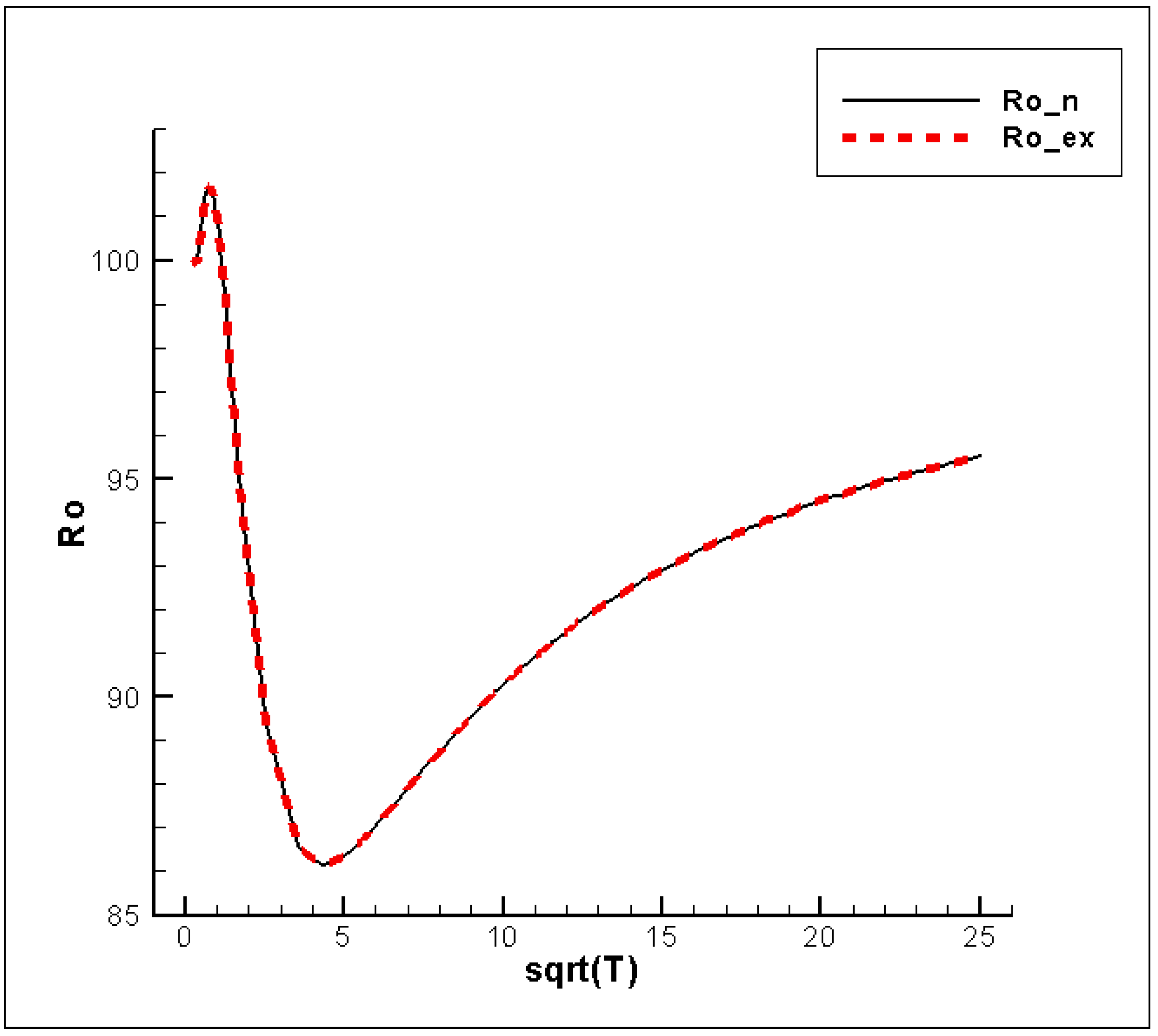
Figure 4 shows an image demonstrating that the proposed algorithm exhibits a high rate of convergence. The value of the functional decreases to the level of , in just 100 iterations. We chose this accuracy for comparison with the results of the work [3]. From the data in Table 1, it can be seen that the value of the functional is rapidly decreasing.
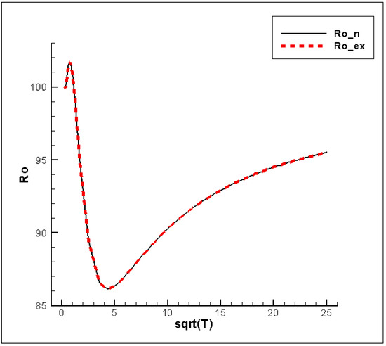
Figure 4.
Comparison of graphs of exact and approximate solutions of apparent resistance.

Table 1.
Numerical results of solving the inverse problem.
The differential evolution method provides high convergence in solving the inverse MTS problem due to its ability to globally optimize complex and multimodal functions. The convergence criteria used, such as changing the values of the objective function and changing the population, ensure that the solutions found are close to the global optimum, which is especially important when working with multi-layer models in MTS [36].
The differential evolution (DE) method is highly resistant to interference in the input data when solving the inverse problem of magnetotelluric sensing (MTS). This stability is related to its stochastic nature and the ability to optimize globally. The DE uses a population of potential solutions, which allows the algorithm to be less sensitive to noise in the data [36]. The mutation and crossover stage helps to create a variety of solutions that can smooth out the effects of interference. Random components in the process of mutation and crossover provide exploration of various regions of the solution space, which helps to avoid the traps of local minima caused by noise. The selection process at each step ensures that only the best solutions that minimize the target function are preserved, which reduces the impact of abnormal data.
5. Mathematical Formulation of the Inverse Problem for a Single-Layer Medium
For a single-layer medium, it is possible to consider the following formulation of the inverse problem. The equations for the and components lead to the solution of the direct MTS problem [13]:
where is the one-dimensional distribution of specific electrical resistances in the section, is the conductivity of the medium.
In mathematical geophysics, it is customary to distinguish two main tasks; the direct one, in which the theoretical electromagnetic field is calculated using a given model, and the inverse one, in which the parameters of the medium are determined using the model field.
Therefore, by specifying additional information
the inverse problem (50)–(53) can be obtained. The coefficient is found from the condition of the minimum functional
5.1. The Method of Conjugate Equations for the Inverse MTS Problem
The inverse problem (50)–(53) is solved by the optimal control method. It is required to find a control for the problem (50)–(52), which delivers a minimum to the functional (54).
The variation of the functional has the form
by introducing the notation , the following will be obtained
Consider the formulation of the perturbed problem to the problem (50)–(52):
To formulate the problem related to , we subtract the system of Equations (55)–(57) from the system of Equations (50)–(52). As a result, the following relations will be obtained:
By considering the expression (58) and multiplying by an arbitrary function , by integrating resulting expression by and after that, the following expression will appear:
Given the boundary conditions (59) and (60), the following expressions will be obtained:
By definition, the main part of the functional increment is the gradient
and then the formulation of the conjugate problem and the gradient of the functional will be as follows:
5.2. Algorithm for Solving the Inverse Problem with the Landweber Method
1. The initial approximation is ;
2. Solution of the direct problem (50)–(52) according to ;
3. Calculation of according to the Formula (54);
4. Solution of the conjugate problem (61)–(63) according to ;
5. Calculation of the gradient of the functional by the Formula (64);
6. Finding the next approximation and switching to 2.
5.3. Numerical Experiments
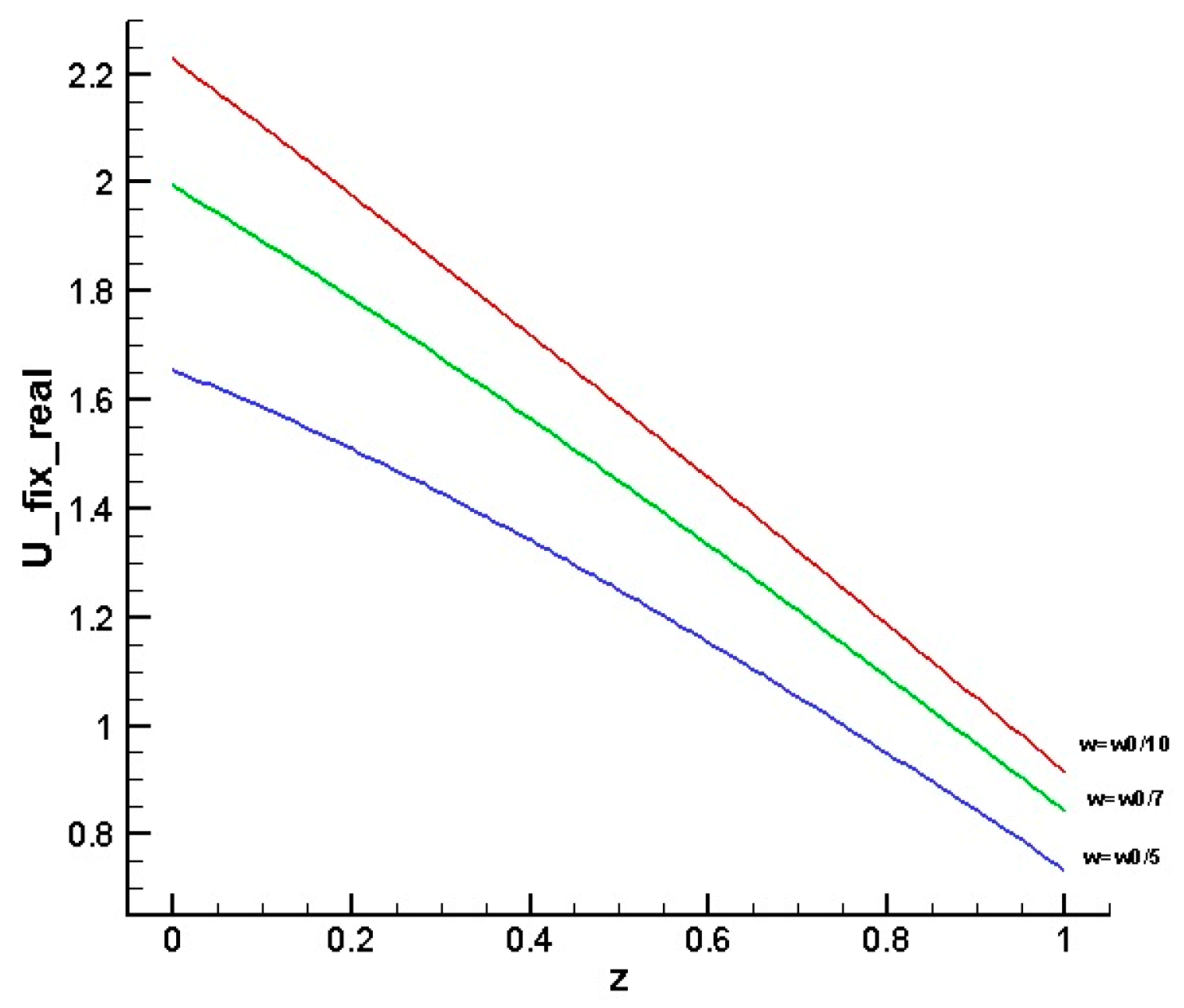
Computational experiments have been carried out for the direct problem at different values
where [13].
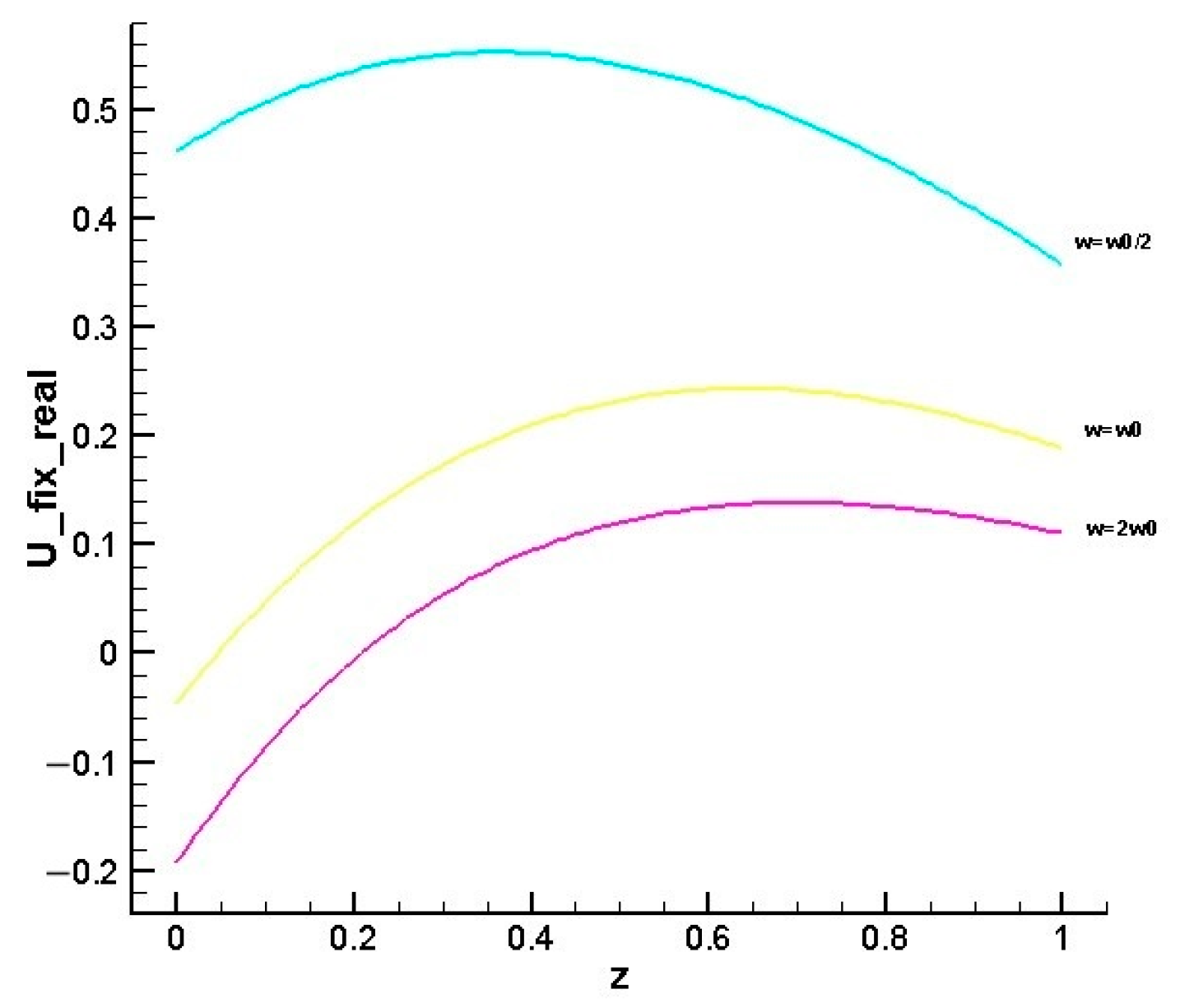
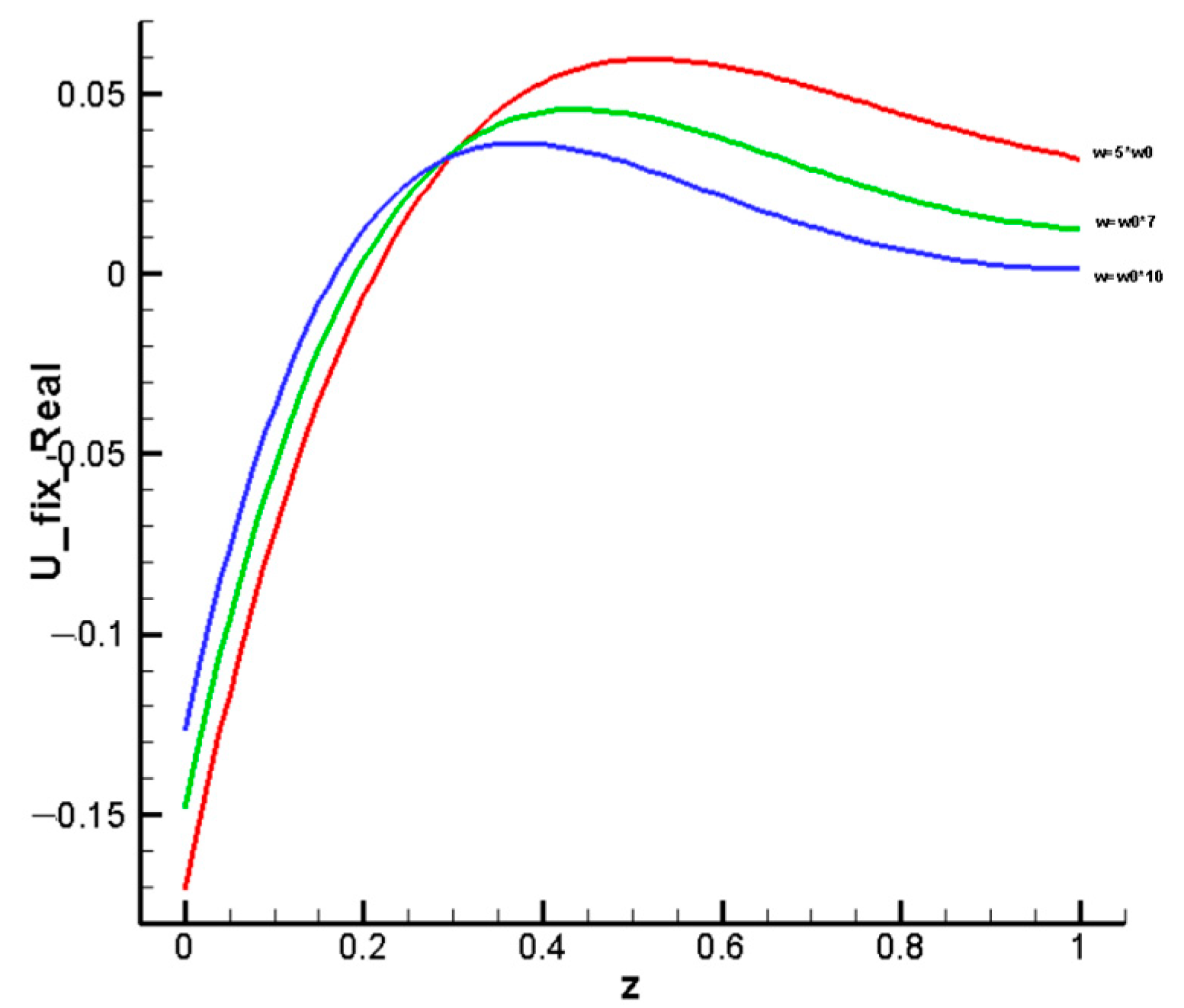
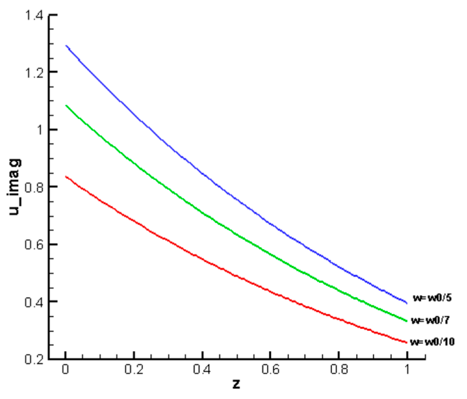
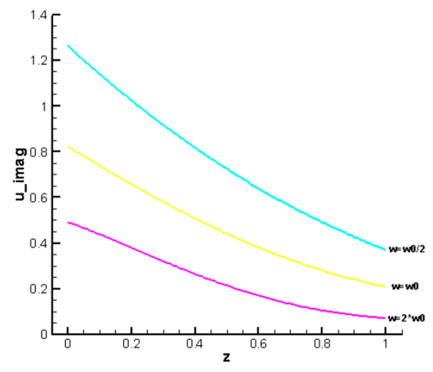
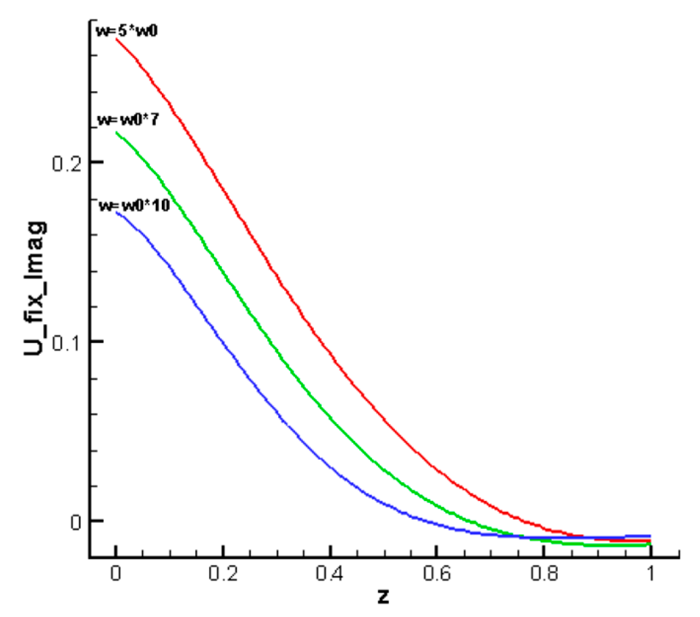
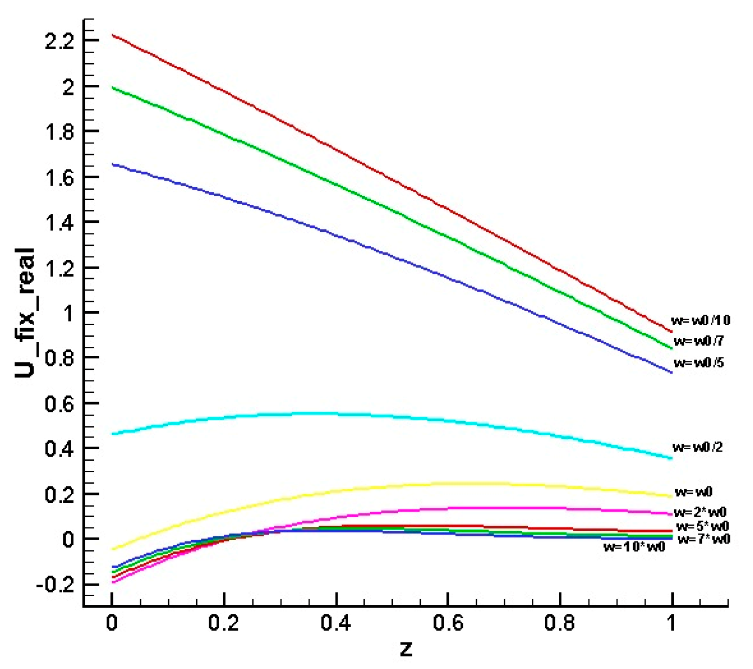
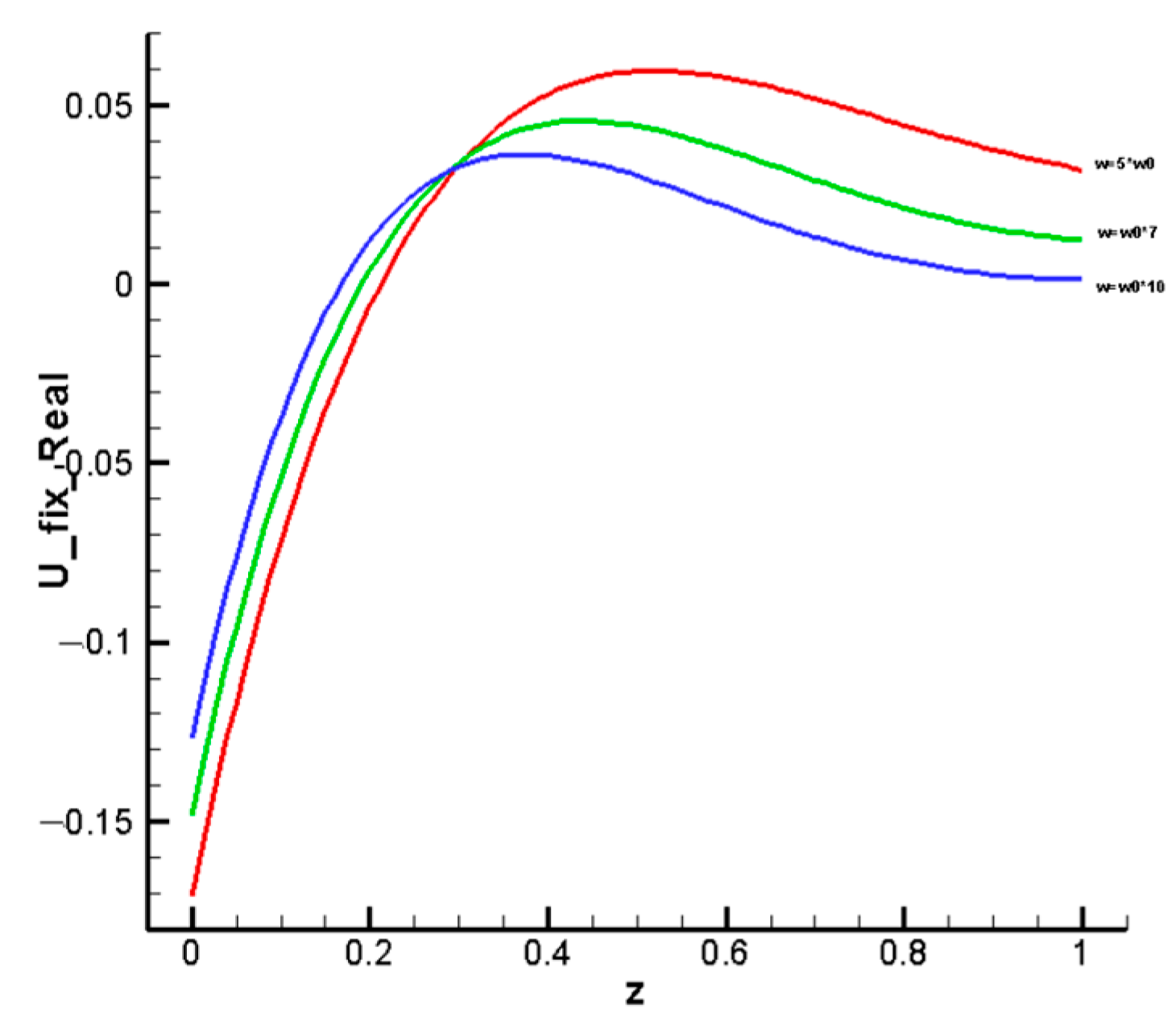
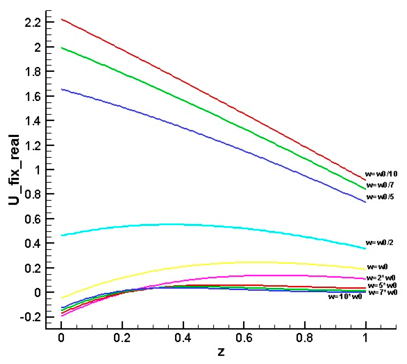
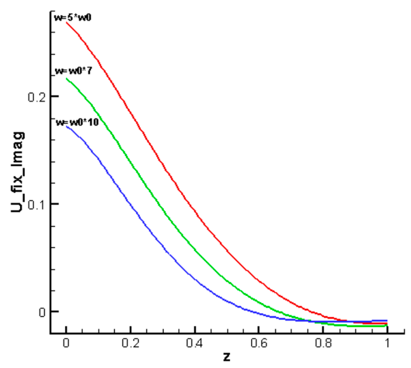
Figure 5, Figure 6 and Figure 7 show graphs of the real parts of the complex function for solving a direct problem, and Figure 8, Figure 9 and Figure 10 show imaginary parts. As can be seen from the graphs, with increasing frequency, the difference in the values of the function decreases. The imaginary part of the function decreases monotonously in all cases.
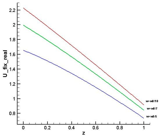
Figure 5.
Graph of the real part of the solution for .
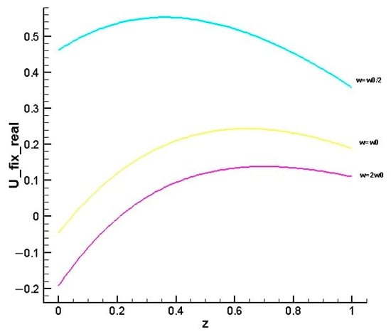
Figure 6.
Graph of the real part of the solution for .
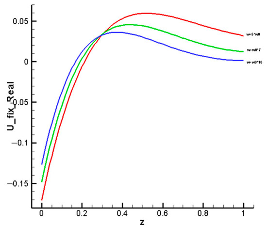
Figure 7.
Graph of the real part of the solution for .
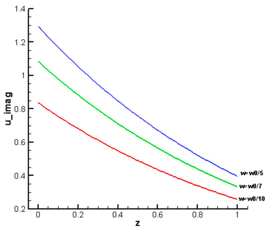
Figure 8.
Graph of the imaginary part of the solution for .
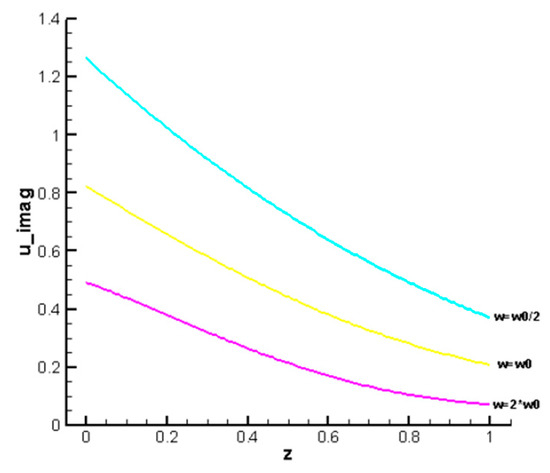
Figure 9.
Graph of the imaginary part of the solution for .
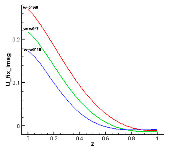
Figure 10.
Graph of imaginary part of the solution for .
The inverse MTS problem is numerically solved by the Landweber’s iterative method. It is necessary to restore the value of the conductivity coefficient of the medium. The initial approximation is given. Figure 11 and Figure 12 show graphs of the solution of the inverse problem based on the restored values of the medium conductivity, and Figure 13 and Figure 14 show graphs of the exact solution, the function.
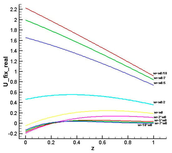
Figure 11.
Graph of the real part .
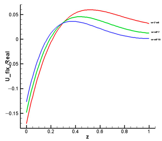
Figure 12.
Graph .

Figure 13.
Graph of the exact solution .
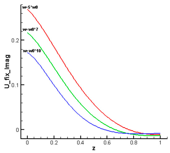
Figure 14.
Graph of the exact solution .
As can be seen from Table 2, 276 iterations were performed, while the value of the functional decreased by 30.562283 times, and the norm of the difference between the exact and approximate values of the medium conductivity coefficient takes the value .
Table 2.
Results of numerical calculations of the inverse problem.
In the Landweber method, the use of minimization of the quadratic functional with conjugate optimization methods makes it possible to achieve high accuracy of solutions due to the effective use of gradient information and faster convergence to a minimum. The Landweber method is known for its ability to efficiently search for solutions in the parameter space, which makes it possible to more accurately reconstruct the distribution of parameters in single-layer models. The use of the quadratic functional simplifies calculations, as it allows linear approximation of changes in the objective function, which reduces computational costs.
6. Conclusions
The magnetotelluric sounding method is one of the classical methods of electrical research aimed at studying the alternating electromagnetic field caused by magnetospheric and ionospheric activity in order to obtain information about the structure of the upper layers of the Earth. The theoretical foundations of the MTS method are based on systems of Maxwell’s equations that describe the electromagnetic field. Maxwell’s equations in classical form are four differential equations describing the laws of conservation of charge and electromagnetic induction. This article studied the relationship between magnetic variations and Earth currents based on the system of Maxwell’s equations. In the framework of the study, the Earth was considered to consist of horizontal layers with different electrical resistance, while the resistance inside each layer is considered constant, and the resistance of the upper half-space (air) is infinite.
It was proposed to solve stationary and non-stationary MTS problems using the quaternionic Fourier transform. The use of QFT makes it possible to exclude one of the spatial and temporal variables, leading to a more convenient form of solution. The application of quaternion Fourier transforms in time translates the original problem into the frequency domain, which allows for a more in-depth investigation of its nature. In the frequency domain, it becomes more clear to identify the main components of the signal and their interactions, which allows a deeper analysis of the physical aspects of the task.
The numerical solution of the direct problem of magnetotelluric sounding has shown that at relatively high frequencies the function significantly depends on the properties of the upper layers of the section and at low frequencies, on deeper horizons. Conclusions from the results of the numerical solution of the inverse problem associated with a multi-layer structure have confirmed that the differential evolution method is a very effective tool for global minimization of the objective function.
The Landweber method, based on minimizing the quadratic function using conjugate optimization methods, has been applied to solve inverse problems in single-layer MTS domains. For the case of a single-layer medium, the boundary conditions used provide all possible options for modeling the process. This makes it possible to model the field in single-layer areas with a realistic interpretation of surface and deep boundaries and their applicability to real geophysical scenarios. The Landweber method demonstrates improved accuracy and high computational efficiency. These advantages make it the preferred choice for solving complex MTS tasks, providing more accurate and efficient restoration of the parameters of geophysical models.
Author Contributions
Conceptualization, S.E.K. and N.M.T.; methodology, S.E.K., N.M.T. and L.N.T.; software, Z.E.D. and L.N.T.; validation, S.E.K., Z.E.D. and L.N.T.; formal analysis, S.E.K. and L.N.T.; investigation, Z.E.D. and L.N.T.; resources, S.E.K., Z.E.D. and L.N.T.; data curation, S.E.K. and Z.E.D.; writing—original draft preparation, Z.E.D.; writing—review and editing, L.N.T.; visualization, L.N.T.; supervision, N.M.T.; project administration, S.E.K. and N.M.T.; funding acquisition, N.M.T. All authors have read and agreed to the published version of the manuscript.
Funding
The research is funded by the Committee of Science of the Ministry of Higher Education and Science of the Republic of Kazakhstan (AP14871252 “Construction and research of quaternion Fourier transforms and their application in the creation of information systems for problems of geophysics and geochemistry”).
Data Availability Statement
All data generated or analyzed during this study are included in this published article.
Conflicts of Interest
The authors declare no conflicts of interest.
References
- Berdichevsky, M.N.; Dmitriev, V.I. Magnetotellurgical Sounding of Horizontally Homogeneous Media; Nedra: Moscow, Russia, 1992; 351p. [Google Scholar]
- Kashafutdinov, O.V. Substantiation of Direct and Inverse Problems of Magnetotelluric Sounding (MTS) and Experiments to Solve Them; INM SO RAN: Krasnoyarsk, Russia, 2005; 83p. [Google Scholar]
- Krasnov, I.K.; Zubarev, K.M.; Ivanova, T.L. Numerical solution of the problem of restoring electrophysical parameters based on the results of sounding and alternating current. Math. Model. Numer. Methods 2018, 58, 475–487. [Google Scholar]
- Urynbassarova, D.; Urynbassarova, A. Hybrid Transforms; IntechOpen: London, UK, 2023. [Google Scholar] [CrossRef]
- Urynbassarova, D.; Teali, A.A. Convolution, Correlation, and Uncertainty Principles for the Quaternion Offset Linear Canonical Transform. Mathematics 2023, 11, 2201. [Google Scholar] [CrossRef]
- Alekseeva, L.A. Biquaternion generalizations of Maxwell’s and Dirac’s equations and properties of their solutions. J. Probl. Evol. Open Syst. 2023, 24, 91–101. [Google Scholar] [CrossRef]
- Alexeyeva, L.A. Generalized Solutions of Stationary Boundary Value Problems for Biwave Equations. Differ. Equ. 2022, 58, 475–487. [Google Scholar] [CrossRef]
- Bahri, M.; Ashino, R.; Vaillancourt, R. Continuous quaternion fourier and wavelet transformations. Int. J. Wavelets Multiresolution Inf. Process. 2014, 12, 1460003. [Google Scholar] [CrossRef]
- Bahri, M.; Ashino, R.; Vaillancourt, R. Two-dimensional quaternion wavelet transform. Appl. Math. Comput. 2011, 218, 10–21. [Google Scholar] [CrossRef]
- Bahri, M.; Hitzer, E.S.M.; Hayashi, A.; Ashino, R. An uncertain principle for quaternion Fourier transform. Comput. Math. Appl. 2008, 56, 2398–2410. [Google Scholar] [CrossRef]
- Tikhonov, A.N. On determining electrical characteristics of the deep layers of the Earth’s crust. Dokl. Akad. Nauk. SSSR 1950, 73, 295–297. [Google Scholar]
- Cagniard, L. Basic theory of the magneto-telluric method of geophysical prospecting. Geophysics 1953, 18, 605–635. [Google Scholar] [CrossRef]
- Dedok, V.A.; Karchevsky, A.L.; Romanov, V.G. Numerical method for determining the dielectric constant modulo the vector of the electric intensity of the electromagnetic field. Sib. J. Ind. Math 2019, 22, 48–58. [Google Scholar] [CrossRef]
- Kabanikhin, S.I.; Lorenzi, A. An identification problem related to the integrodifferent Maxwell’s equation. Inverse Probl. 1991, 7, 863. [Google Scholar] [CrossRef]
- Kasenov, S.; Nurseitova, A.; Nurseitov, D. A conditional stability estimate of continuation problem for the Helmholtz equation. AIP Conf. Proc. 2016, 1759, 020119. [Google Scholar]
- Shishlenin, M.A.; Kasenov, S.E.; Askerbekova, Z.A. Numerical algorithm for solving the inverse problem for the Helmholtz equation. In Proceedings of the 9th International Conference on CITech 2018, Ust-Kamenogorsk, Kazakhstan, 25–28 September 2018; Communications in Computer and Information Science. Springer: Berlin/Heidelberg, Germany, 2019; Volume 998, pp. 197–207. [Google Scholar]
- Newman, G.A.; Alumbaugh, D.L. Three-dimensional magnetotelluric inversion using non-linear conjugate gradients. Geophys. J. Int. 2000, 140, 410–424. [Google Scholar] [CrossRef]
- Rodi, W.; Mackie, R.L. Nonlinear conjugate gradients algorithm for 2-D magnetotelluric inversion. Geophysics 2001, 66, 174–187. [Google Scholar] [CrossRef]
- Isaev, I.; Obornev, E.; Obornev, I.; Shimelevich, M.; Dolenko, S. Neural network recognition of the type of parameterization scheme for magnetotelluric data. In Advances in Neural Computation, Machine Learning, and Cognitive Research II: Selected Papers from the XX International Conference on Neuroinformatics; Springer International Publishing: Moscow, Russia, 2019; pp. 176–183. [Google Scholar]
- Obornev, E.; Obornev, I.; Rodionov, E.; Shimelevich, M. Application of Neural Networks in Nonlinear Inverse Problems of Geophysics. Comput. Math. Math. Phys. 2020, 60, 1025–1036. [Google Scholar] [CrossRef]
- Isaev, I.; Obornev, I.; Obornev, E.; Rodionov, E.; Shimelevich, M.; Dolenko, S. Neural network recovery of missing data of one geophysical method from known data of another one in solving inverse problems of exploration geophysics. In Proceedings of the 6th International Workshop on Deep Learning in Computational Physics, Dubna, Russia, 6–8 July 2022; p. 18. [Google Scholar]
- Deng, F.; Hu, J.; Wang, X.; Yu, S.; Zhang, B.; Li, S.; Li, X. Magnetotelluric Deep Learning Forward Modeling and Its Application in Inversion. Remote Sens. 2023, 15, 3667. [Google Scholar] [CrossRef]
- Temirbekov, N.; Kasenov, S.; Berkinbayev, G.; Temirbekov, A.; Tamabay, D.; Temirbekova, M. Analysis of Data on Air Pollutants in the City by Machine-Intelligent Methods Considering Climatic and Geographical Features. Atmosphere 2023, 14, 892. [Google Scholar] [CrossRef]
- Constable, S.C.; Parker, R.L.; Constable, C.G. Occam’s inversion: A practical algorithm for generating smooth models from electromagnetic sounding data. Geophysics 1987, 52, 289–300. [Google Scholar] [CrossRef]
- de Groot-Hedlin, C.; Constable, S.C. Occam’s inversion to generate smooth, two-dimensional models from magnetotelluric data. Geophysics 1990, 55, 1613–1624. [Google Scholar] [CrossRef]
- Smith, J.T.; Booker, J.R. Rapid Inversion of two and three dimensional magnetotelluric data. J. Geophys. Res. 1991, 96, 3905–3922. [Google Scholar] [CrossRef]
- Tikhonov, A.N. Mathematical Geophysics; Publishing House of the Joint Institute of Earth’s Physics of RAS: Moskow, Russia, 1999; 476p. [Google Scholar]
- Polyakova, N.S. Differentiation of functions of a quaternion variable. Chebyshevsky Collect. 2019, 20, 298–310. [Google Scholar]
- Ell, T.A.; Le Bihan, N.; Sangwine, S.J. Quaternion Fourier Transforms for Signal and Image Processing; Wiley-ISTE; John Wiley & Sons: New York, NY, USA, 2014; 160p. [Google Scholar]
- Tikhonov, A.N.; Lipskaya, N.V.; Deniskin, N.A.; Nikiforova, N.N.; Lomakina, Z.D. On electromagnetic sounding of the deep layers of the Earth. Rep. Acad. Sci. Russ. Acad. Sci. 1961, 140, 587–590. [Google Scholar]
- Baigereyev, D.; Kasenov, S.; Temirbekova, L. Empowering geological data analysis with specialized software GIS modules. Indones. J. Electr. Eng. Comput. Sci. 2024, 34, 1953–1964. [Google Scholar] [CrossRef]
- Krivorotko, O.I.; Kabanikhin, S.I.; Bektemesov, M.A.; Sosnovskaya, M.I.; Neverov, A.V. Simulation of COVID-19 Spread Scenarios in the Republic of Kazakhstan Based on Regularization of the Agent-Based Model. J. Appl. Ind. Math. 2023, 17, 94–109. [Google Scholar] [CrossRef]
- Temirbekova, L.N.; Dairbaeva, G. Gradient and direct method of solving Gelfand-Levitan integral equation. Appl. Comput. Math. 2013, 12, 234–246. [Google Scholar]
- Temirbekov, N.; Imangaliyev, Y.; Baigereyev, D.; Temirbekova, L.; Nurmangaliyeva, M. Numerical simulation of inverse geochemistry problems by regularizing algorithms. Cogent Eng. 2022, 9, 2003522. [Google Scholar] [CrossRef]
- Temirbekov, N.M.; Los, V.L.; Baigereyev, D.R.; Temirbekova, L.N. Module of the geoinformation system for analysis of geochemical fields based on mathematical modeling and digital prediction methods, News of the academy of sciences of the republic of Kazakhstan. Ser. Geol. Tech. Sci. 2021, 5, 137–145. [Google Scholar] [CrossRef]
- Storn, R.; Price, K. Differential Evolution—A Simple and Efficient Heuristic for Global Optimization over Continuous Spaces. J. Glob. Optim. 1997, 11, 341–359. [Google Scholar] [CrossRef]
Disclaimer/Publisher’s Note: The statements, opinions and data contained in all publications are solely those of the individual author(s) and contributor(s) and not of MDPI and/or the editor(s). MDPI and/or the editor(s) disclaim responsibility for any injury to people or property resulting from any ideas, methods, instructions or products referred to in the content. |
© 2024 by the authors. Licensee MDPI, Basel, Switzerland. This article is an open access article distributed under the terms and conditions of the Creative Commons Attribution (CC BY) license (https://creativecommons.org/licenses/by/4.0/).