Numerical Simulation and Comparison of Different Steady-State Tumble Measuring Configurations for Internal Combustion Engines

Abstract

To enhance air–fuel mixing and turbulence during combustion, spark ignition internal combustion engines commonly employ tumble vortices of the charge inside the cylinder. The intake phase primarily dictates the generated tumble, which is influenced by the design of the intake system. Utilizing steady-state flow rigs provides a practical method to assess an engine’s cylinder head design’s tumble-generating characteristics. This study aims to conduct computational fluid dynamics (CFD) numerical simulations on various configurations of steady-state flow rigs and compare the resulting tumble ratios. The simulations are conducted for different inlet valve lifts of a four-valve cylinder head with a shallow pent-roof. The findings highlight variations among these widely adopted configurations.

1. Introduction

In addition to ongoing efforts to electrify the fleet of light-duty vehicles, spark ignition (SI) internal combustion (IC) engines still dominate the market, and their power density, efficiency, and emissions are still improving. Furthermore, the potential use of alternative CO₂-neutral fuels, such as biofuels [1,2,3], synthetic fuels (e-fuels) [4], or even hydrogen [5,6,7] may extend the lifespan of SI engines used in passenger cars and light commercial vehicles. In-cylinder charge motion plays a pivotal role in controlling fuel–air mixing and the combustion process both in SI engines [8] and compression ignition (CI) engines [9,10]. It also significantly influences engine heat transfer [11]. While swirling flow is preferred in CI engines, SI engines usually utilize a tumbling motion of the mixture within the cylinder. That flow pattern enhances the turbulence energy inside the combustion chamber, thereby increasing burning speed, improving idle stability and exhaust gas recirculation (EGR) tolerance [12,13]. Tumble also regulates fuel stratification in gasoline direct injection (GDI) engines [14,15].

The design of inlet ports and cylinder head significantly influences the air–fuel flow pattern within the combustion chamber. While the flow field in the cylinder can be visualized in laboratory engines that allow for optical access, with the use of, i.e., laser diagnostic techniques, those methods demand substantial resources and costly equipment. Experiments under firing conditions are feasible, but the complexities and constraints associated with combustion make it far easier to conduct cold flow measurements [16]. A practical alternative to measure the tumble motion creating ability of a cylinder head design is employing a steady-state tumble measuring flow rig. These methods offer the added benefit of quite straightforward examination of the flow in production engine cylinder heads. These rigs can also facilitate in-cylinder velocity field particle image velocimetry (PIV) measurements [12,17,18]. The more commonly used “integral” methods evaluate the tumble strength by measuring the flux of angular momentum. This is achieved using a paddle wheel or an impulse torque meter [19,20,21,22,23]. However, the absence of a standardized testing procedure for quantifying tumble intensity leads to non-directly comparable results from existing methods, rendering their outcomes more “relative” than “absolute”. Xu [24] provides a comprehensive summary of such steady flow testing arrangements.

Computational fluid dynamics (CFD) is a convenient as well as reliable tool for the investigation of the flow field in the combustion chamber of an engine. Many studies compare experimental data of tumble ratios with results obtained from CFD simulations [16,19,21,25,26,27,28]. CFD simulations offer a convenient way to compare results for various cylinder head configurations, expediting the optimization of the geometry. However, in a CFD study, certain associated issues require special attention, such as careful selection of the numerical methods, numerical grid, and turbulence models used. Furthermore, it is essential to establish a correlation between the tumble ratios measured using various steady-state flow rigs and the charge motion inside the cylinder under firing or motoring conditions.

This study compares computational fluid dynamics (CFD) simulation data regarding the tumble ratio and flow coefficient, for a modern cylinder head with four valves, employing different steady-state flow rigs, across varying valve lifts. These numerical simulation findings will aid in establishing correlations with experimental measurements acquired through different steady-state tumble measurement flow rigs.

2. Materials and Methods

Steady-state flow benches, employed to measure the tumble generating capacity of a given intake system in an internal combustion (IC) engine, typically utilize either an impulse swirl meter that measures the torque applied by the flow or a paddle wheel that measures rotational speed of the flow. Impulse swirl meters are considered more precise because of issues related to mechanical reliability and flow disruption the paddle wheel causes. Impulse flow meters comprise a honeycomb-type flow straightener, positioned downstream the cylinder head. Initially designed for the measurement of the in-cylinder swirl, these techniques have been modified to measure tumble, through the use of a suitable tumble adaptor. One commonly used tumble adaptor, employed to convert tumbling air motion into swirl, which can be measured by one of the described devices, was developed by Ricardo [29]. There are two variations of this adaptor: the “T-type” and the “L-type” (Figure 1). In the “T-type” setup, air exits from both directions of the adaptor tube, exhibiting symmetry when the valve lift of both inlet valves is equal. Angular momentum is measured inside the one of the exit tubes, thus constituting half of the total angular momentum. In the “L-type” setup, the tumble adapter tube is closed on one side, and all the airflow passes through the swirl meter. In both configurations, the tube’s diameter (D) is approximately equal to the bore (B) of the cylinder, with typical tube lengths (L) ranging around 500 mm. Although neither dimension is deemed critical due to angular momentum conservation, it is worth noting that wall friction inside the tumble adapter tube slightly affects the measurements. The distance between the tube axis and the cylinder head (H) is a crucial dimension influencing tumble measurement. Ricardo’s method employees a distance of H = B/2 + 20 mm. Both configurations are depicted in Figure 1.

To achieve a steady-state flow within the test rig, a constant pressure difference is applied. This pressure difference is carefully chosen to ensure fully turbulent flow, and is typically determined by the Reynolds number, which is evaluated using the inner seat diameter of the intake valve. For cylinder head geometries relative with automotive engines, typical values for the pressure difference lies between 400 and 1000 mm H₂O.

The Ricardo method calculates the discharge coefficient C_d and the flow coefficient C_f and as follows ([20]):

$${\mathrm{C}}_{\mathrm{f}}=\frac{\dot{\mathrm{Q}}}{{\mathrm{A}}_{\mathrm{in}.\mathrm{seat}}·{\mathrm{V}}_{\mathrm{o}}} {\mathrm{C}}_{\mathrm{d}}=\frac{\dot{\mathrm{Q}}}{{\mathrm{A}}_{\mathrm{v}}·{\mathrm{V}}_{\mathrm{o}}}$$

(1)

The non-dimensional tumble number N_T-R is calculated by the following ([20]):

$${\mathrm{N}}_{\mathrm{T-R}}=\frac{8\mathrm{G}}{\dot{\mathrm{m}}·{\mathrm{V}}_{\mathrm{o}}·\mathrm{B}}$$

(2)

G is the torque that is measured, $\dot{\mathrm{m}}$ is the air mass flow rate, $\dot{\mathrm{Q}}$ is the air volume flow rate, B is the bore of the cylinder, A_in.seat is the inner seat area of the valve, A_v is the orifice area between the valve head and the valve seat area, and V_o is the velocity head $\left(\sqrt{2\Delta \mathrm{P}/\mathsf{\rho }}\right)$. If only half of the torque is measured (as in the “T-type” tumble adaptor), only half of the total mass flow rate should be used for in the denominator of Equation (2).

Another widely used method is the FEV (“Forschungsgesellschaft für Energietechnik und Verbrennungsmotoren” in German) steady-state flow rig (Figure 2). According to this method, the cylinder head is mounted on a cylinder, which is equipped with a rotating paddle ring. The tumbling motion of the flow rotates the paddle ring and exits the cylinder through the two symmetric side openings. Those two openings also accommodate the mounting of the ring’s shaft. The diameter of those two openings, according to the specifications of this method, is 0.35∙B, where B is the diameter of the cylinder, which is significantly smaller that the of the Ricardo tumble adaptor. It is thus anticipated that for a fixed pressure drop, the flow rate through the rig would be lower than that of the Ricardo method. An advantage of this method over the Ricardo method is that a real piston can be placed in the bottom of the dummy cylinder, and thus how its shape influences the generated tumble can be assessed.

The non-dimensional rig tumble number N_T-FEV is usually calculated as the ratio of velocities C_T/C_A, where C_T is the circumferential velocity of the tumbling motion in the mean paddle radius R_MPR, and C_A is the axial velocity in the cylinder.

$${\mathrm{N}}_{\mathrm{T-FEV}}=\frac{{\mathrm{C}}_{\mathrm{T}}}{{\mathrm{C}}_{\mathrm{A}}}=\frac{2·\mathsf{\pi }·\mathrm{N}·{\mathrm{R}}_{\mathrm{MPR}}}{{\mathrm{C}}_{\mathrm{A}}}$$

(3)

where N is the rotation speed of the paddle wheel and R_MPR is the mean paddle wheel radius, which, according to the rig’s specifications, is R_MPR = 0.36375∙B. The axial velocity in the cylinder can be calculated as ${\mathrm{C}}_{\mathrm{A}}=\dot{\mathrm{m}}/\left({\mathsf{\rho }}_{\mathrm{cyl}}·{\mathrm{A}}_{\mathrm{v}}\right)$, where $\dot{\mathrm{m}}$ is mass flow rate, ρ_cyl is the air density inside the cylinder, and A_v is the orifice area between the valve head and the valve seat.

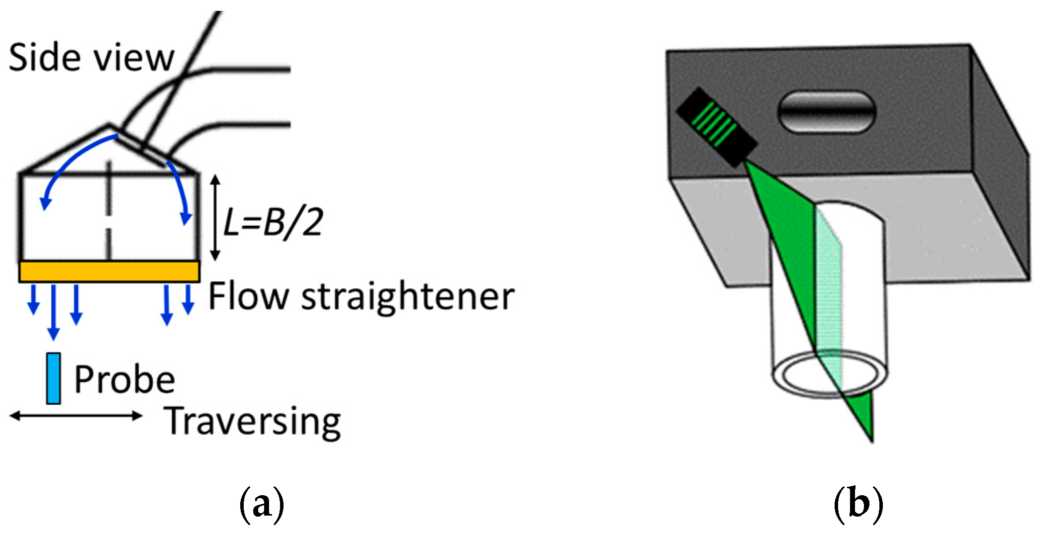
Beside the above-described experimental configurations, which are used to determine integral flow parameters, other velocity measuring or flow visualization techniques are also used such as or particle image velocimetry (PIV) [16,17,18,20] or hot-wire anemometry (HWA). Usual configurations are shown in Figure 3. In the HWA method, a flow straightener is placed at the exit of the cylinder, and the axial velocity component is measured just after this straightener. In the PIV method, a transparent cylinder is used, particles are seeded in the flow, and the detailed flow field is measured in the symmetry plane perpendicular to the tumble rotation axis (and possibly also in other parallel planes). The flow exits from one or two side ports, similarly to the FEV method. In all those methods, the detailed velocity field measured can be integrated in order to extract integral flow features, as tumble strength.

The purpose of this study is to numerically simulate the above steady-state measuring methods and compare the results obtained. A 3D parametric model for the inlet valves, ports, and cylinder head was constructed using suitable CAD software (Autodesk Fusion v2.0, Figure 4). This design incorporates straight inlet ports, a shallow combustion chamber with a minimal pent roof angle, moderately sized squish zones, and large intake and exhaust valves. This arrangement exhibits a strong resemblance to the configuration of a recently developed high-power output SI engine. The exhaust side was not modelled.

Table 1. Dimensions of the simulated cylinder head geometry.

Stroke (mm)	89.7
Bore (mm)	87.5
Pentroof angle (deg)	17°
Diameter of inlet valves (mm)	32
Angle of valve’s seat (deg)	45°

shows the principal dimensions of the geometry.

To facilitate the application of proper boundary conditions in the CFD simulation, an inlet plenum chamber was added before the inlet port and an outlet plenum chamber was added after the exit tube. For all configurations except the Ricardo L-tube, only half of the complete geometry was modeled due to the presence of a symmetry plane. The computational domains for all simulated cases are illustrated in Figure 5 and Figure 6.

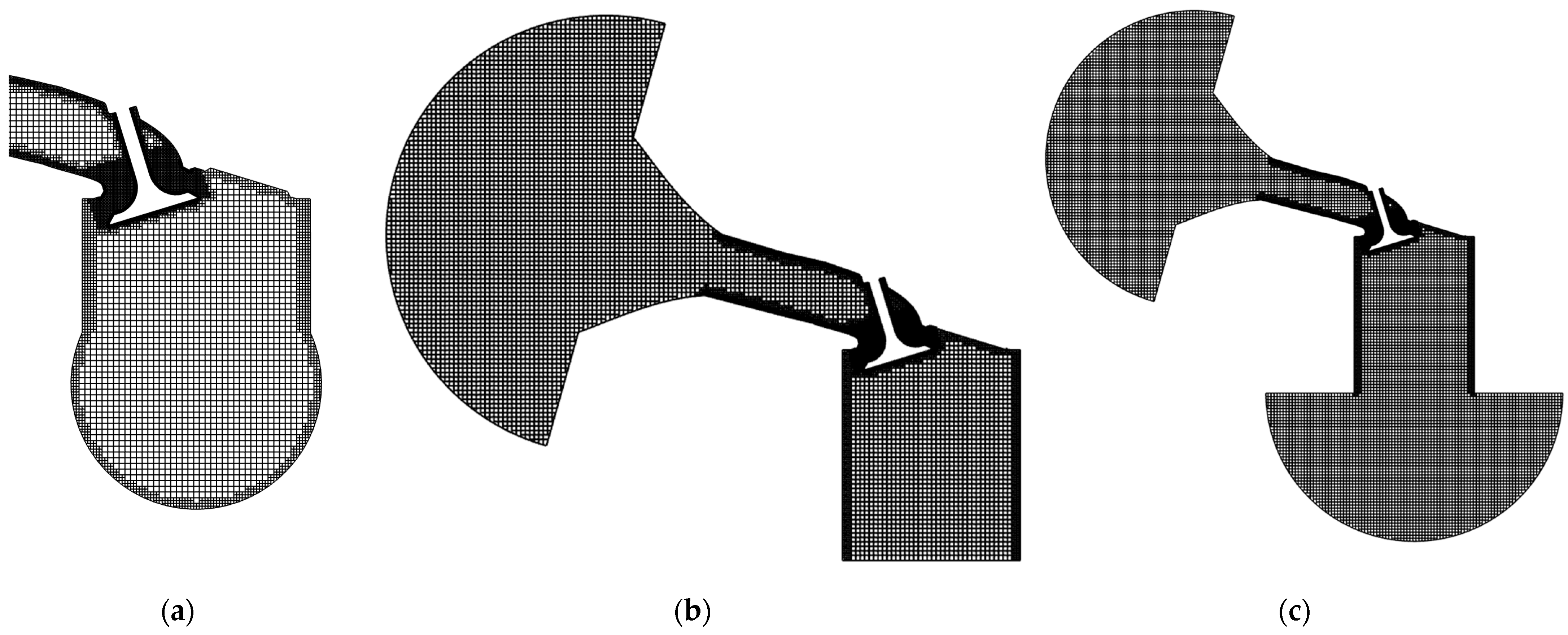
This investigation employed the CONVERGE CFD software (v3.1.5) for numerical simulations [30]. CONVERGE utilizes a fully automated cut-cell meshing technique to generate an orthogonal, body-fitted, computational mesh. The software embeds the geometry surface inside a Cartesian mesh block and subsequently trims the cells at their intersection points with the surface, ensuring a close fit to the complex geometry. In a previous numerical study of similar configurations [31], it was found that a base mesh with uniform cells with 2 mm edge length, with 1 level of mesh refinement at the cylinder’s walls, an exit tube, and 3 successive levels of mesh refinement around the valves and the valve opening region gives adequately accurate results. The total number of cells for the Ricardo T-tube tumble adapter is around 1.2 M cells (for the half model) and for the Ricardo T-tube tumble adapter around 2 M cells. The numerical grid used for the simulations is presented in Figure 7.

The numerical mesh did not incorporate the impulse honeycomb swirl meter employed within the tumble adaptors for either Ricardo configuration. The torque exerted by the flow on the swirl meter was instead determined by calculating the angular momentum flux, measured parallel to the tube’s axis and relative to the cross-section’s center. For the FEV case, the paddle wheel is also not modeled in the simulations. The tumble ratio is calculated from the angular momentum of the flow inside the cylinder. For the HWA case, porous media are placed at the exit of the cylinder in order to simulate the flow straightener present in the experimental setup. For this case, the tumble ratio is calculated from the angular momentum flux in the surface between the cylinder and the flow straightener region.

In a previous numerical study of a similar configuration [31], various RANS turbulence models and convective schemes were tested using several numerical mesh densities. The use of the k-ω SST turbulence model ([32]) and second-order upwind (SOU) convective scheme produced the most consistent results for the various cases considered. These are the models also used in this study.

3. Results

3.1. Flow Coefficients and Tumble Ratios

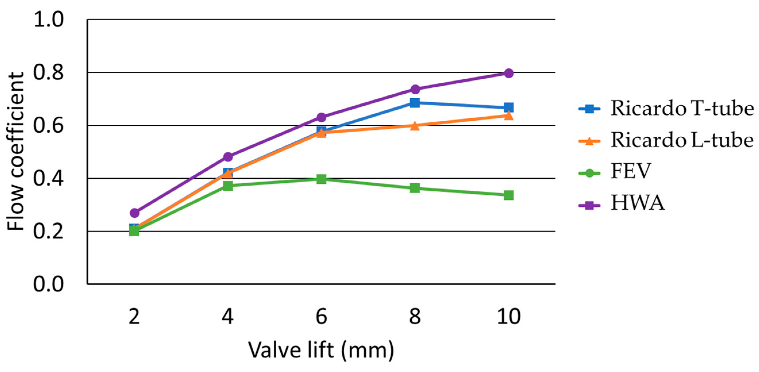
For all configurations considered, simulations were performed for 2, 4, 6, 8, and 10 mm valve lifts. The upstream gauge pressure was set at 600 mm H₂O. Figure 8 presents a comparison of the predicted flow coefficients (Equation (1)). It is clear that for the FEV method and for valve lifts larger than 4 mm, the flow is significantly restricted by the small diameter of the exit tube (Figure 2). Simulations with lower upstream gauge pressure or shorter length of the exit tube did not affect significantly the predicted flow coefficient. Increasing the diameter of the exit tube did lead to increased flow rates. It is anticipated that in the real experimental configuration, the presence of the rotating paddle wheel inside the cylinder will further reduce the flow rate. In the HWA configuration, although the presence of the porous media flow straightener does cause a small pressure drop, the absence of any exit tubes leads to an increased flow rate, compared with the two Ricardo configurations. For that case, the absence of any significant organized rotating flow inside the cylinder (as it will be shown later in this text) further attributes to this result. Comparing the two Ricardo configurations, for small valve lifts, the flow rates predicted are very close, while for larger valve lifts, the presence of two exit tubes of the T-tube configuration lead to an increased flow rate. For all cases, but especially for the Ricardo and the FEV configurations, the flow rate is also affected by the flow pattern inside the cylinder and the presence of organized large-scale vortices.

Figure 9 shows the comparison of the predicted tumble ratios. For the FEV configuration, the tumble number is calculated using Equation 3, but since there is not a real rotating paddle wheel inside the computational domain and the angular momentum is calculated inside the whole volume of the cylinder, the mean radius used in Equation (3) was R_MPR = 0.5∙B. The corresponding paddle wheel speed N of the experimental configuration was approximated by the angular speed of the flow around the horizontal axis through the center of mass of the cylinder (the axis of the exit tube in Figure 6a, axis Y in our simulation).

$${\mathsf{\omega }}_{\mathrm{Y}}=\frac{{\mathrm{L}}_{\mathrm{Y}}}{{\mathrm{I}}_{\mathrm{Y}}}$$

(4)

where I_Y and L_Y are the moment of inertia and the angular momentum, respectively, around that axis. These can be calculated using the following summations over the numerical cells inside the computational region of the cylinder:

$${\mathrm{L}}_{\mathrm{Y}}=\sum _{\mathrm{n}=1}^{\mathrm{total} \mathrm{cells}}\left\{{\mathrm{m}}_{\mathrm{n}}\left[\left({\mathrm{z}}_{\mathrm{n}}-{\mathrm{z}}_{\mathrm{cm}}\right){\mathrm{u}}_{\mathrm{n}}-\left({\mathrm{x}}_{\mathrm{n}}-{\mathrm{x}}_{\mathrm{cm}}\right){\mathrm{w}}_{\mathrm{n}}\right]\right\}$$

(5)

$${\mathrm{I}}_{\mathrm{Y}}=\sum _{\mathrm{n}=1}^{\mathrm{total}\mathrm{cells}}\left\{{\mathrm{m}}_{\mathrm{n}}\left[{\left({\mathrm{z}}_{\mathrm{n}}-{\mathrm{z}}_{\mathrm{cm}}\right)}^2-{\left({\mathrm{x}}_{\mathrm{n}}-{\mathrm{x}}_{\mathrm{cm}}\right)}^2\right]\right\}$$

(6)

m_n is the mass inside computational cell n; x_n and z_n are the coordinates of the corresponded cell’s center; x_cm and z_cm are the coordinates of the center of mass, which is the assumed rotation center; and u_n and w_n are the velocities in the X and Z directions.

For the two Ricardo configurations, the respective tumble number is calculated using Equation (2), where the torque G measured in the experimental setup is replaced by the angular momentum (around the tube’s axis) flux through the surface between Section 1 and Section 2 inside the exit tube. In the “T-type”, the mass flow rate in the denominator of Equation (2) should be half of the total. For the HWA configuration, the corresponding tumble ratio is calculated again by Equation (2) using the angular momentum (around Y axis) flux leaving the cylinder and entering the porous media region.

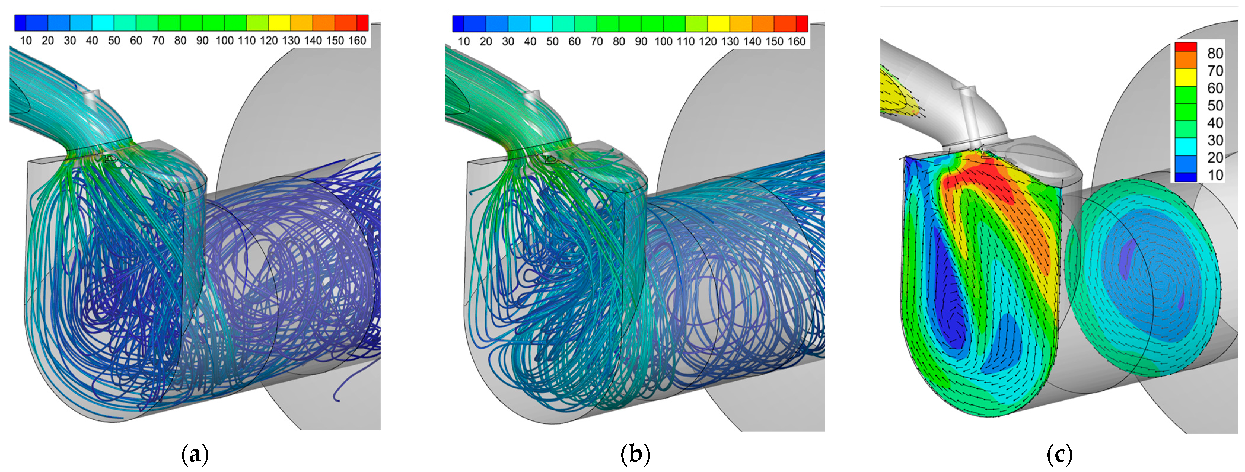
As can be seen in Figure 9, although the tumble ratios are calculated using different method for each configuration, they are quite similar, with the exception of the HWA configuration for low valve lifts. Figure 10, Figure 11, Figure 12 and Figure 13 show the flow field inside each configuration, for 4, 8, and 10 mm valve lifts.

3.2. HWA Configuration

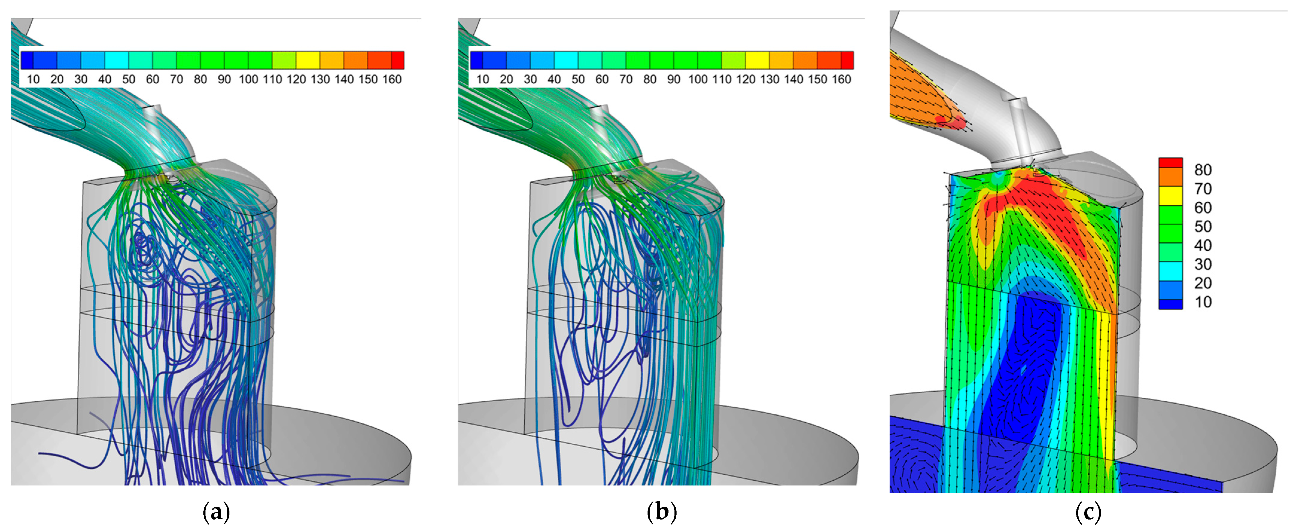
For the HWA configuration (Figure 10) it is obvious that there is not any significant large scale horizontal vortex present, and the angular momentum flux around the Y-axis is calculated from the non-uniformity of the axial velocities. As can be seen in Figure 11b, for higher flow rates (large valve lifts), the flow exits the front side of the valve seat region (the side towards the center of the cylinder) with higher velocities. A strong flow jet emerging from the front side of the valve seat opening is, to an extent, a desirable feature, if a tumbling motion inside the cylinder is to be created. However, in the case of the HWA configuration, the absence of a wall in the other end of the cylinder does not promote the creation of a large-scale horizontal vortex. In that sense, the HWA configuration can be considered as an “indirect” method, as it actually measures the non-uniformity of the axial velocity field and not the strength of any generated horizontal vortex. It is, however, remarkable that the HWA calculated tumble ratios for higher valve lifts that are actually quite close to the calculated tumble ratios of the other configurations. For lower valve lifts though, due to lower flow rates, the velocity of the flow emerging from the backside of the valve seat is almost as high as on the front side (Figure 11a). A weak vortex is formed beneath the valve (Figure 10a), and the flow remains attached to the backside of the cylinder sidewalls. The velocities at the plane of the flow straightener entrance are stronger on the backside, and thus the tumble ratio calculated for low valve lifts indicates a reverse rotation in the flow (negative tumble ratios in Figure 9).

3.3. Ricardo T-Tube and L-Tube Configurations

When examining the Ricardo L-tube and T-tube configurations for lower valve lifts (up to 6 mm), it becomes apparent that the flow coefficient for both configurations remains nearly identical, exhibiting a marginal increase with a diminishing rate (Figure 8). This suggests that the mass flow at lower valve lifts is primarily influenced by the decreased flow area within the seating region rather than the downstream flow structure. Additionally, for these valve lifts, there is a gradual rise in the tumble number. Notably, the predicted tumble numbers for the T-tube tend to be slightly elevated. However, for increased valve lifts, distinct trends are seen. For the T-tube configuration, the flow coefficient demonstrates a continuous increase up to a valve lift of 8 mm, followed by a decline at a 10 mm lift, signifying a reduction in the effective mass flow rate through the apparatus. Conversely, the L-tube configuration displays a sustained increase, albeit at a notably slower pace. At a valve lift of 8 mm, the predicted tumble number for the L-tube significantly surpasses that of the T-tube configuration (Figure 9). Despite appearing unusual, this behavior aligns with the variations observed in the flow coefficient. Increased tumble motion might lead to a decrease in mass flow. These observations suggest that, for large valve lifts, the flow coefficient is primarily governed by the flow dynamics within the cylinder rather than the valve lift itself. Notably, at a valve lift of 8 mm, the two configurations exhibit divergent behaviors. A closer inspection of the predicted flow fields (Figure 12 and Figure 13) provide some insight for this behavior. For the L-tube configuration, most of the fluid entering the cylinder heads towards the single side exit of the rig, and there is no flow symmetry around the vertical midplane of the cylinder, as is the case in the T-tube configuration. This reduces the size and strength of the counter rotating vortices beneath the inlet valves, leaving more space for the main central rotating vortex to grow stronger inside the cylinder (Figure 13b). Within the T-tube configuration, lower valve lifts result in the high-velocity flow entering from the backside of the inlet valves to generate secondary counter-rotating vortices beneath the valves. For this configuration, the flow symmetry around the vertical midplane of the cylinder promotes the existence of these structures.

At larger valve lifts (10 mm), the secondary vortices within the T-tube configuration diminish significantly. The flow structure then transitions to resemble that observed in the L-tube configuration, characterized by a dominant, horizontally oriented vortex positioned near the cylinder’s center. This shift in the T-tube’s in-cylinder flow pattern, from 8 mm to 10 mm valve lift, coincides with a predicted reduction in the flow coefficient and an increase in the tumble number. Conversely, the L-tube configuration for 8 mm valve lift exhibits a well-organized and stronger primary vortex within the cylinder (Figure 13b). This feature contributes to a lower predicted mass flow rate and a higher tumble number compared to the T-tube configuration at the same valve lift.

3.4. FEV Configuration

In the FEV configuration, for small valve lifts up to 4 mm, the high velocities at the backside of the valve opening, in conjunction with the placement of the small-diameter exit tube vertically at the center of the cylinder, allow for the counter-rotating vortices beneath the inlet valves to grow in size (Figure 14a). The center vortex is small and pushed at the side of the cylinder. This flow pattern leads to a flow coefficient comparable with the two Ricardo configurations and slightly lower tumble ratio for a 4 mm valve lift. For lifts above 4 mm, the small diameter of the exit tube restricts the flow, causing the creation of a very well-defined center-rotating vortex, which is very well aligned with the axis of the exit tube (Figure 14b,c). The presence of this strong vortex together with the small diameter of the exit tube cause a drop in the flow coefficient, and for lifts above 6 mm, the actual flow rate decreases. On the other hand, the tumble ratio increases with a faster rate, compared with the Ricardo configurations.

As can be seen in Figure 9, although the tumble ratios for each configuration are calculated using different method, the tumble ratios of the FEV configuration are directly comparable with those obtained from the Ricardo configurations, even though the flow coefficient for that configuration is significantly lower, especially for larger valve lifts. Although that seems odd, it is actually anticipated because the tumble ratio is not a measure of the absolute angular momentum, but rather the ratio of the angular momentum to the axial momentum of the flow. For the FEV configuration, the resulting lower mass flow rate leads to lower angular momentum (nominator of Equation (3)), but also to a lower axial momentum (denominator of Equation (3)).

4. Discussion

Modern spark ignition (SI) engines prioritize in-cylinder tumbling motion for optimal charge flow. However, the lack of a standardized and universally accepted testing procedure for quantifying tumble intensity hinders direct comparison of results obtained from existing methods. Consequently, these methods yield findings with relative, rather than absolute, validity. Numerical simulations applied to four such experimental approaches effectively illustrate the discrepancies within the internal cylinder flow field. Notably, these simulations reveal variations in both flow coefficients and the resulting flow rates. On the other hand, although the configurations are very different and the tumble ratios for these cases are calculated using different methods, the values obtained are quite close to each other, especially for higher inlet valve lifts. A close examination of the predicted flow fields reveals the cause of the differences.

The HWA experimental configuration—which is not an integral method, such as the Ricardo and the FEV, but requires the measurement of the velocity field at several points downstream the cylinder—is quite different from the other two methods. The experimental apparatus does not allow for the creation of a strong tumbling vortex. Thus, the flow field inside the cylinder of the experimental setup has rather small relevance to the real in-cylinder flow. The tumble ratio is actually calculated from the non-uniformity of the axial velocities. Although the tumble ratio for small valve lifts are quite different compared with the other methods, for inlet valve lifts larger than 6 mm, the ratios calculated are surprisingly close to those of the other configurations.

In the FEV configuration, the small diameter of the exit tube and the resulting strong tumbling vortex that is generated lowers the flow rate, especially for larger valve lifts. The tumble ratio for lifts larger than 4 mm shows an almost linear increase, indicating that the flow pattern does not change, having a very well-defined strong tumbling vortex inside the cylinder. The flow rate for the two variations of the Ricardo method is not choked by the exit tube, as in the FEV case. On the other hand, the FEV configuration offers the possibility to perform test using different piston crown shapes and examine how these influence the tumble inside the cylinder. This is not possible for the Ricardo configurations, which have the disadvantage that the flow field and the tumbling vortex strength and location are affected by the half-cylinder shape present in the place where there would normally be a piston. The differences in the flow coefficient and the tumble ratio between the two variants of the Ricardo method, the L-tube and the T-tube configurations, are caused by the fact that in the latter case, the flow field is not symmetrical relative to the vertical symmetry plane between the two inlet valves, because the whole flow entering from both valves heads toward the side of the exit tube. At low inlet valve lifts, there are extended counter-rotating vortices underneath the two inlet valves and a relative weak and confined main tumble vortex, while at larger lifts, the main tumble vortex expands and becomes stronger, while the vortices underneath the valves diminish. The existence or non-existence of symmetry affects the point where the flow transitions from one pattern to the other.

5. Conclusions

This study employed computational fluid dynamics (CFD) simulations to analyze the steady-state flow characteristics within a modern spark ignition (SI) engine cylinder head using four commonly utilized steady-state flow rigs designed for tumble measurement. The simulations were conducted across a range of valve lift settings. The three more commonly used configurations, Ricardo (T-tube and L-tube) and FEV, fall in the category of “integral” methods. The fourth configuration simulated (HWA) requires the integration of the optically measured velocities at point locations.

Although the tumble ratios are calculated using different method for each configuration, they are quite similar, with the exception of the HWA configuration for low valve lifts. A close examination of the predicted flow fields reveals the cause of the differences. Each experimental method has advantages and disadvantages. The most important are the following:

• The Ricardo L-tube configuration generates a non-symmetrical flow field inside the cylinder even if the cylinder head and the inlet valve lifts are symmetrical.
• Both Ricardo configurations, in place of the piston, have the exit tubes’ bottom side, which affects the angular momentum of the flow.
• The FEV configuration is technically more demanding than the Ricardo configurations, having the rotating paddle wheel inside the cylinder. The use of the rotating paddle wheel has also the disadvantage that affects the flow field. The small diameter of the exit tube restricts the flow. On the other hand, it allows for the use of a real production piston and can assess how its crown shape affects the tumble.
• All integral methods can be effectively used only when the axis of the tumbling flow inside the cylinder is parallel with the exit tubes or the axis of the rotating paddle wheel. That is not always the case (i.e., when the lift of the inlet valves is not equal or one of the inlet valves is deactivated).
• HWA measurements for tumble ratio estimation require more expensive equipment and effort. The flow field inside the cylinder in regions away from the cylinder head is not relevant with the flow field inside the cylinder of a motored engine.

As a closing remark, it should be noted that the next step for completing this evaluation between the configurations under investigation should be a comparison with results from the simulation of the cold flow intake stroke, either with fixed inlet valves lift or with realistic valve lift profiles. This would reveal how relevant these steady-state measuring configurations are with a real in-cylinder flow field.

References

1. Ibham, V.; Mohd Farid Muhamad, S.; Mohd Azman, A.; Zulkarnain Abdul, L.; Mohd Rozi Mohd, P.; Djati Wibowo, D.; Djamari, D.W. Future Direction of Microalgae Biodiesel in Indonesia. J. Adv. Res. Appl. Sci. Eng. Technol. 2021, 25, 1–6. [Google Scholar] [CrossRef]
2. Gheidan, A.A.S.; Abdul Wahid, M.; Abdul Munir, F.; Anthony Chukwunonso, O. Feasibility Study of Bio-fuel As a Sustainable Product of Biomass: An Overview of Its Fundamentals, Application and Environmental Impact. J. Adv. Res. Fluid Mech. Therm. Sci. 2021, 88, 106–122. [Google Scholar] [CrossRef]
3. Mohsin, R.; Majid, Z.A.; Shihnan, A.H.; Nasri, N.S.; Sharer, Z.; Mat, R.C. Effects of Multi-Variant Biofuel on Engine Performance and Exhaust Emission of DDF Engine System. J. Adv. Res. Fluid Mech. Therm. Sci. 2020, 6, 1–18. [Google Scholar]
4. Wouters, C.; Lehrheuer, B.; Pischinger, S.; Seifert, P.; Raabe, T.; Kolbeck, M.; Rausch, B.; Menger, L.; Kulzer, A.C. Evaluation of Synthetic Gasoline Fuels and Alcohol Blends in a Spark-Ignition Engine. SAE Int. J. Fuels Lubr. 2022, 15, 333–347. [Google Scholar] [CrossRef]
5. Shadidi, B.; Najafi, G.; Yusaf, T. A Review of Hydrogen as a Fuel in Internal Combustion Engines. Energies 2021, 14, 6209. [Google Scholar] [CrossRef]
6. Sementa, P.; de Vargas Antolini, J.B.; Tornatore, C.; Catapano, F.; Vaglieco, B.M.; Sánchez, J.J.L. Exploring the potentials of lean-burn hydrogen SI engine compared to methane operation. Int. J. Hydrogen Energy 2022, 2, 5044–5056. [Google Scholar] [CrossRef]
7. Mat Taib, N.; Abu Mansor, M.R.; Wan Mahmood, W.M.F. Simulation of Hydrogen Fuel Combustion in Neon-oxygen Circulated Compression Ignition Engine. J. Adv. Res. Numer. Heat Transf. 2020, 3, 25–36. [Google Scholar] [CrossRef]
8. Hill, P.G.; Zhang, D. The effects of swirl and tumble on combustion in spark-ignition engines. Prog. Energy Combust. Sci. 1994, 20, 373–429. [Google Scholar] [CrossRef]
9. Yoon, S.; Lee, S.; Kwon, H.; Lee, J.; Park, S. Effects of the swirl ratio and injector hole number on the combustion and emission characteristics of a light duty diesel engine. Appl. Therm. Eng. 2018, 142, 68–78. [Google Scholar] [CrossRef]
10. Wang, G.; Yu, W.; Li, X.; Yang, R. Influence of fuel injection and intake port on combustion characteristics of controllable intake swirl diesel engine. Fuel 2020, 262, 116548. [Google Scholar] [CrossRef]
11. Heywood, J. Internal Combustion Engine Fundamentals; McGraw-Hill Education: Berkshire, UK, 2018. [Google Scholar]
12. Kim, M.J.; Lee, S.H.; Kim, W.T. Correlation study of the measured tumble ratios using three different methods: Steady flow rig; 2-dimensional PIV; and 3-dimensional PTV water flow rig. Int. J. Automot. Technol. 2006, 7, 441–448. [Google Scholar]
13. Kaplan, M. Influence of swirl, tumble and squish flows on combustion characteristics and emissions in internal combustion engine-review. Int. J. Automot. Eng. Technol. 2019, 8, 83–102. [Google Scholar] [CrossRef]
14. Duronio, F.; Vita, A.D.; Allocca, L.; Anatone, M. Gasoline direct injection engines—A review of latest technologies and trends. Part 1: Spray breakup process. Fuel 2020, 265, 116948. [Google Scholar] [CrossRef]
15. Saw, O.P.; Addepalli, S.K.; Mallikarjuna, J.M. (Eds.) Effects of Cylinder Head Geometry on Mixture Stratification, Combustion and Emissions in a GDI Engine—A CFD Analysis. International Powertrains, Fuels & Lubricants Meeting; SAE International: Warrendale PA, USA, 2019. [Google Scholar]
16. Jamil, A.; Baharom, M.B.; Aziz, A.R.A. IC engine in-cylinder cold-flow analysis—A critical review. Alex. Eng. J. 2021, 60, 2921–2945. [Google Scholar] [CrossRef]
17. El Adawy, M.; Heikal, M.R.; A Aziz, A.R. Experimental Investigation of the In-Cylinder Tumble Motion inside GDI Cylinder at Different Planes under Steady-State Condition using Stereoscopic-PIV. J. Appl. Fluid Mech. 2019, 12, 41–49. [Google Scholar] [CrossRef]
18. El Adawy, M.; Heikal, M.R.; Aziz, A.A.R.; Siddiqui, M.; Munir, S. Characterization of the Inlet Port Flow under Steady-State Conditions Using PIV and POD. Energies 2017, 10, 1950. [Google Scholar] [CrossRef]
19. Mohammadebrahim, A.; Hannani, S.; Shafii, M. Investigation into the effect of intake port geometric parameters and blockage on flow coefficient and in-cylinder flow: Application to engine port design. Sci. Iran. 2014, 21, 438–448. [Google Scholar]
20. El-Adawy, M.; Heikal, M.R.; Aziz, A.R.A.; Siddiqui, M.I.; Wahhab, H.A.A. Experimental study on an IC engine in-cylinder flow using different steady-state flow benches. Alex. Eng. J. 2017, 56, 727–736. [Google Scholar] [CrossRef]
21. Ramajo, D.; Zanotti, A.; Nigro, N. In-cylinder flow control in a four-valve spark ignition engine: Numerical and experimental steady rig tests. Proc. Inst. Mech. Eng. Part D J. Automob. Eng. 2011, 225, 813–828. [Google Scholar] [CrossRef]
22. Ramajo, D.E.; Nigro, N.M. In-Cylinder Flow Computational Fluid Dynamics Analysis of a Four-Valve Spark Ignition Engine: Comparison between Steady and Dynamic Tests. J. Eng. Gas Turbines Power 2010, 132, 052804. [Google Scholar] [CrossRef]
23. Wahono, B.; Setiawan, A.; Lim, O. Effect of the intake port flow direction on the stability and characteristics of the in-cylinder flow field of a small motorcycle engine. Appl. Energy 2021, 288, 116659. [Google Scholar] [CrossRef]
24. Xu, H. (Ed.) Some Critical Technical Issues on the Steady Flow Testing of Cylinder Heads; SAE Technical Paper Series; SAE International: Warrendale PA, USA, 2001. [Google Scholar]
25. Ballapu, H.; Mallikarjuna, J.M. Effect of piston shape on in-cylinder flows and air–fuel interaction in a direct injection spark ignition engine—A CFD analysis. Energy 2015, 81, 361–372. [Google Scholar]
26. Baratta, M.; Misul, D.; Spessa, E.; Viglione, L.; Carpegna, G.; Perna, F. Experimental and numerical approaches for the quantification of tumble intensity in high-performance SI engines. Energy Convers. Manag. 2017, 138, 435–451. [Google Scholar] [CrossRef]
27. Wahono, B.; Setiawan, A.; Lim, O. Experimental study and numerical simulation on in-cylinder flow of small motorcycle engine. Appl. Energy 2019, 255, 113863. [Google Scholar] [CrossRef]
28. Yang, X.; Kuo, T.-W.; Guralp, O.; Grover, R.O.; Najt, P. (Eds.) In-Cylinder Flow Correlations Between Steady Flow Bench and Motored Engine Using Computational Fluid Dynamics. J. Eng. Gas Turbines Power 2017, 139, 072802. [Google Scholar] [CrossRef]
29. Ricardo, J. Steady State Flowbench Port Performance Measurement and Analysis Techniques; Report DP93/0704; 1993. [Google Scholar]
30. Richards, K.J.; Senecal, P.K.; Pomraning, E. CONVERGE 3.0*; Convergent Science: Madison, WI, USA, 2022. [Google Scholar]
31. Theodorakakos, A. Numerical Study of Different Steady-State Flow Rigs for the Tumble Motion Characterization of a Four-Valve Cylinder Head. CFD Lett. 2023, 15, 18–31. [Google Scholar] [CrossRef]
32. Menter, F. (Ed.) Zonal Two Equation k-w Turbulence Models For Aerodynamic Flows. In Proceedings of the 23rd Fluid Dynamics, Plasmadynamics, and Lasers Conference, Orlando, FL, USA, 6–9 July 1993; American Institute of Aeronautics and Astronautics: Reston, VA, USA, 1993. [Google Scholar]
Figure 1. Ricardo tumble adaptor: (a) side view (“T-type” and “L-type”); (b) front view “L-type”; (c) front view “L-type”. The red arrows illustrate the tumbling motion of the flow.
Computation 12 00138 g001
Figure 2. FEV tumble adaptor: (a) side view; (b) front view. The red arrows illustrate the tumbling motion of the flow.
Computation 12 00138 g002
Figure 3. (a) HWA velocity measuring (arrows illustrate the flow field inside the cylinder); (b) PIV velocity measuring.
Computation 12 00138 g003
Figure 4. Different views of the model for the simulated geometry: (a) 3D view; (b) Side view; (c) Top view.
Computation 12 00138 g004
Figure 5. Computational regions for (a) Ricardo T-tube tumble adaptor; (b) Ricardo L-tube tumble adaptor.
Computation 12 00138 g005
Figure 6. Computational domain for (a) FEV tumble adaptor; (b) HWA steady-state measuring configuration.
Computation 12 00138 g006
Figure 7. Cross-section of the computational grid used at the vertical plane bisecting the axis of an inlet valve for each configuration: (a) Ricardo T-tube tumble adaptor; (b) FEV tumble adaptor; (c) HWA steady-state measuring configuration.
Computation 12 00138 g007
Figure 8. Comparison of the predicted flow coefficients for all cases.
Computation 12 00138 g008
Figure 9. Comparison of the predicted tumble ratios for all cases. Note that the tumble ratios for each case are calculated using different methods.
Computation 12 00138 g009
Figure 10. Simulation results for HWA configuration: (a) streamlines for 4 mm valve lift colored by velocity magnitude; (b) streamlines for 8 mm valve lift colored by velocity magnitude; (c) non-dimensional velocity vectors and velocity magnitude contours in the cylinder’s symmetry plane and inside the exit tube, for 10 mm valve lift.
Computation 12 00138 g010
Figure 11. Velocity magnitude contours for the HWA configuration, in a plane parallel to the valve plate in the valve seat region and a horizontal plane neat the flow straightener: (a) 2 mm valve lift; (b) 10 mm valve lift.
Computation 12 00138 g011
Figure 12. Simulation results for the Ricardo T-tube tumble adaptor: (a) streamlines for 4 mm valve lift colored by velocity magnitude; (b) streamlines for 8 mm valve lift colored by velocity magnitude; (c) non-dimensional velocity vectors and velocity magnitude contours in the cylinder’s symmetry plane and inside the exit tube, for 10 mm valve lift.
Computation 12 00138 g012
Figure 13. Simulation results for the Ricardo L-tube tumble adaptor: (a) streamlines for 4 mm valve lift colored by velocity magnitude; (b) streamlines for 8 mm valve lift colored by velocity magnitude; (c) non-dimensional velocity vectors and velocity magnitude contours in the cylinder’s symmetry plane and inside the exit tube, for 10 mm valve lift.
Computation 12 00138 g013
Figure 14. Simulation results for the FEV tumble adaptor: (a) streamlines for 4 mm valve lift colored by velocity magnitude; (b) streamlines for 8 mm valve lift colored by velocity magnitude; (c) non-dimensional velocity vectors and velocity magnitude contours in the cylinder’s symmetry plane and inside the exit tube, for 10 mm valve lift.
Computation 12 00138 g014