Some Aspects of the Effects of Dry Friction Discontinuities on the Behaviour of Dynamic Systems

Abstract

Most studies in the literature consider the value of the coefficient of dynamic friction to be constant. We studied the evolution of a dynamic system when the coefficient of friction results in different values depending on the contact surfaces. A system with four balls fixed on an aluminium plate was driven with constant velocity into motion on the coaxial races of two identical outer bearing rings. The assembly presents a motion with periodic variable amplitude between two extremes, a fact that suggests the presence of a periodical excitation. The test was repeated, but this time, new bodies were used, which were two identical bodies made of two balls rigidised via a short cylindrical rod. When the rings were driven into rotational motion, the two bodies performed different motions; if the bodies were inter-changed, the differences between the motions remained. The rings were analysed, and a small region on the race of one ring was observed, where the roughness was considerably greater than the rest of the surface. Then, a mathematical model for the dynamic system with different friction coefficients was proposed and solved. This model is capable of simulating different situations, such as oscillatory motion and circular motion, with or without separation of the contacting bodies. Here, we present a dynamic model with Hertzian contact points in the presence of dry friction, with the coefficient of friction changing suddenly on the contacting surfaces.

1. Introduction

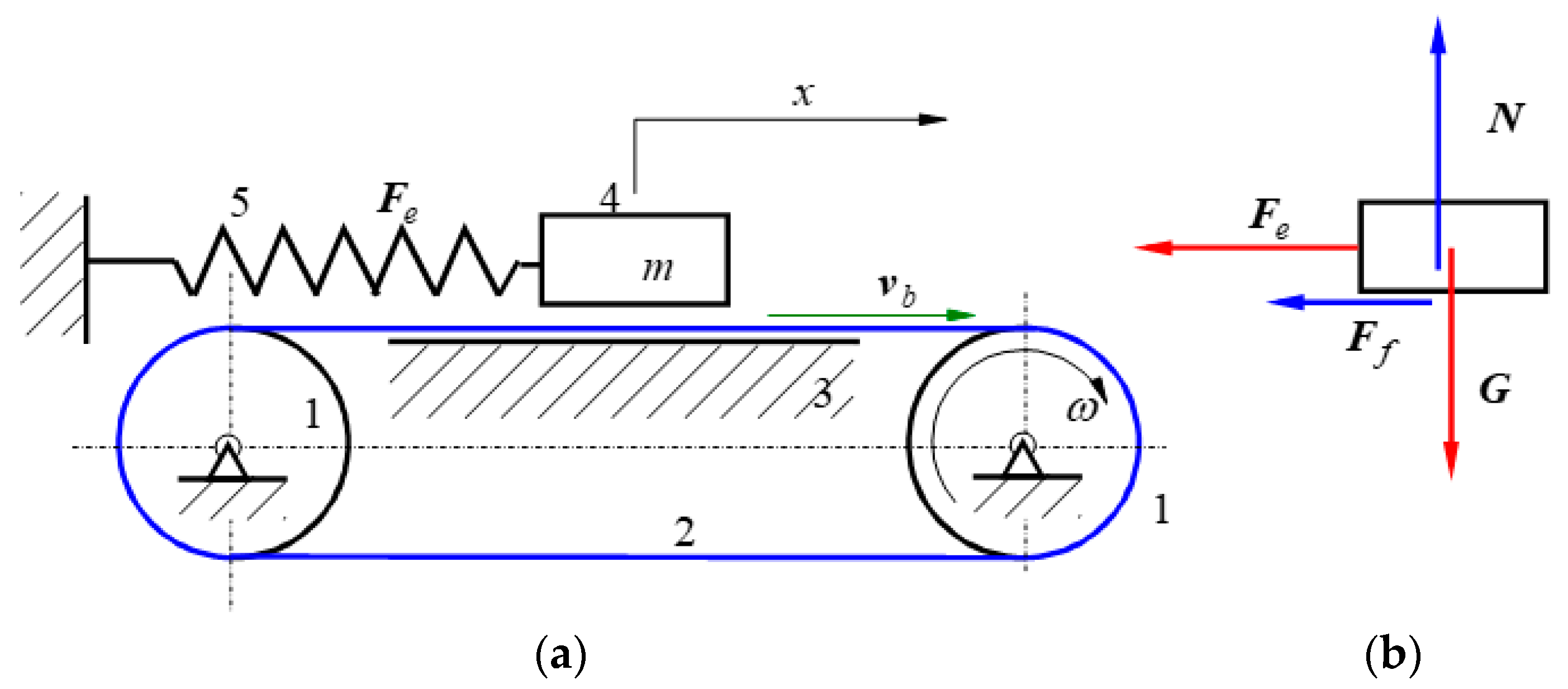
1.1. Classic Dynamic System with Friction

Friction is a phenomenon that occurs continuously in dynamic systems. One of the optimisation criteria in the synthesis of mechanisms consists of avoiding or diminishing shock [1,2]. If we consider cam mechanisms as an example, there are two types of shock: heavy shock, when the velocity of the follower presents finite discontinuities, and soft shock, when the acceleration presents finite discontinuities. Shocks are produced by discontinuities in the tangent and curvature of the cam. An extrapolation of this observation is the question concerning the effect of the friction force discontinuities on the evolution of dynamic systems, considering that the actual boundary surfaces of the elements from a mobile mechanical structure are under continuous change: during operation, deformations, pitting, etc., may occur, which affect well-defined surfaces with different tribological characteristics. The effects of friction can be demonstrated by experimental devices, of which the one presented in Figure 1a is widely used [3,4]. The advantages of using this dynamic system are, firstly, that the fact that the normal reaction has a constant value equal to the weight of the mobile body, and secondly, there is no risk that the constraint is cancelled, as occurs in some dynamic systems with unilateral constraints [5]. The system consists of two identical cylinders (1) with parallel axes that rotate with the same constant angular velocity, $\omega$. A continuous conveyor belt (2) is bent over the cylinders and supported at the upper branch by a horizontal plane part (3) and moves at a constant velocity, $v_b$. A body (4) of mass $m$ is placed on the belt and, therefore, it can move in a horizontal direction, and its position is fully characterised by the linear displacement $x$, resulting in a system with one degree of freedom (1DOF). Dry friction exists between the body and the belt, characterised by the friction force, $F_f\left(v\right)$, where $v$ is the relative velocity between the belt and the body.

$$v=\dot{x}-v_b$$

(1)

The body is connected to the ground by a linear elastic spring (5) with an elastic constant $k_e$. The device has the advantage that for $\omega =0$ and an immobile belt, the mass–spring system performs free damped oscillations, and when $\omega \ne 0$, the belt becomes the excitatory element and the mass–spring system maintains motion. Based on the free body diagram [6] shown in Figure 1b, the equation of motion of the body is obtained as follows:

$$m\ddot{x}=-F_e-F_f$$

(2)

where

$$F_e=k_{e}x; F_f=F_f\left(v\right)$$

(3)

Equation (3) was written under the hypothesis that the reference position $x$ for the displacement of the body corresponds to the undeformed spring. The equation of motion of the body is as follows:

$$m\ddot{x}=-k_{e}x-F_f(\dot{x}-v_b)$$

(4)

An extremely difficult task is choosing an adequate friction model to obtain the law of motion. In the literature, there are numerous friction models that are more or less complex [3,7,8,9]. Marques et al. [3] reviewed the main dry friction models. The earliest and simplest models are due to Amontons [10] and Coulomb [11], according to which the friction force is proportional to the normal reaction and opposes the relative motion. When the relative motion is zero, the function from Figure 2 becomes multi-valued and can take any value within the domain $[-F_c,F_c]$, as shown in the following expression:

$$F_c={\mu }_k{F}_N$$

(5)

where ${\mu }_k$ is the kinetic friction coefficient and $F_N$ is the normal force.

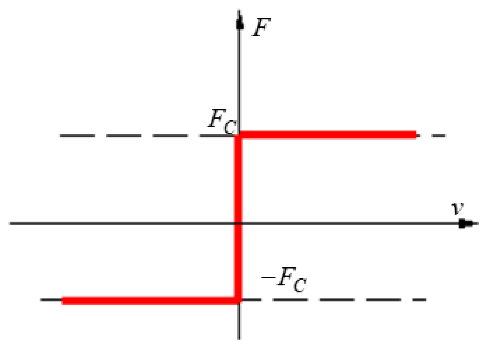
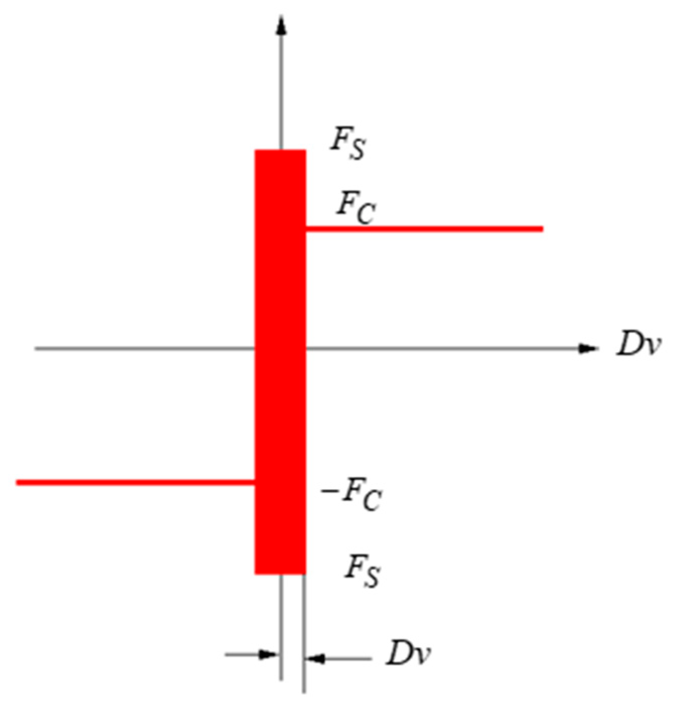
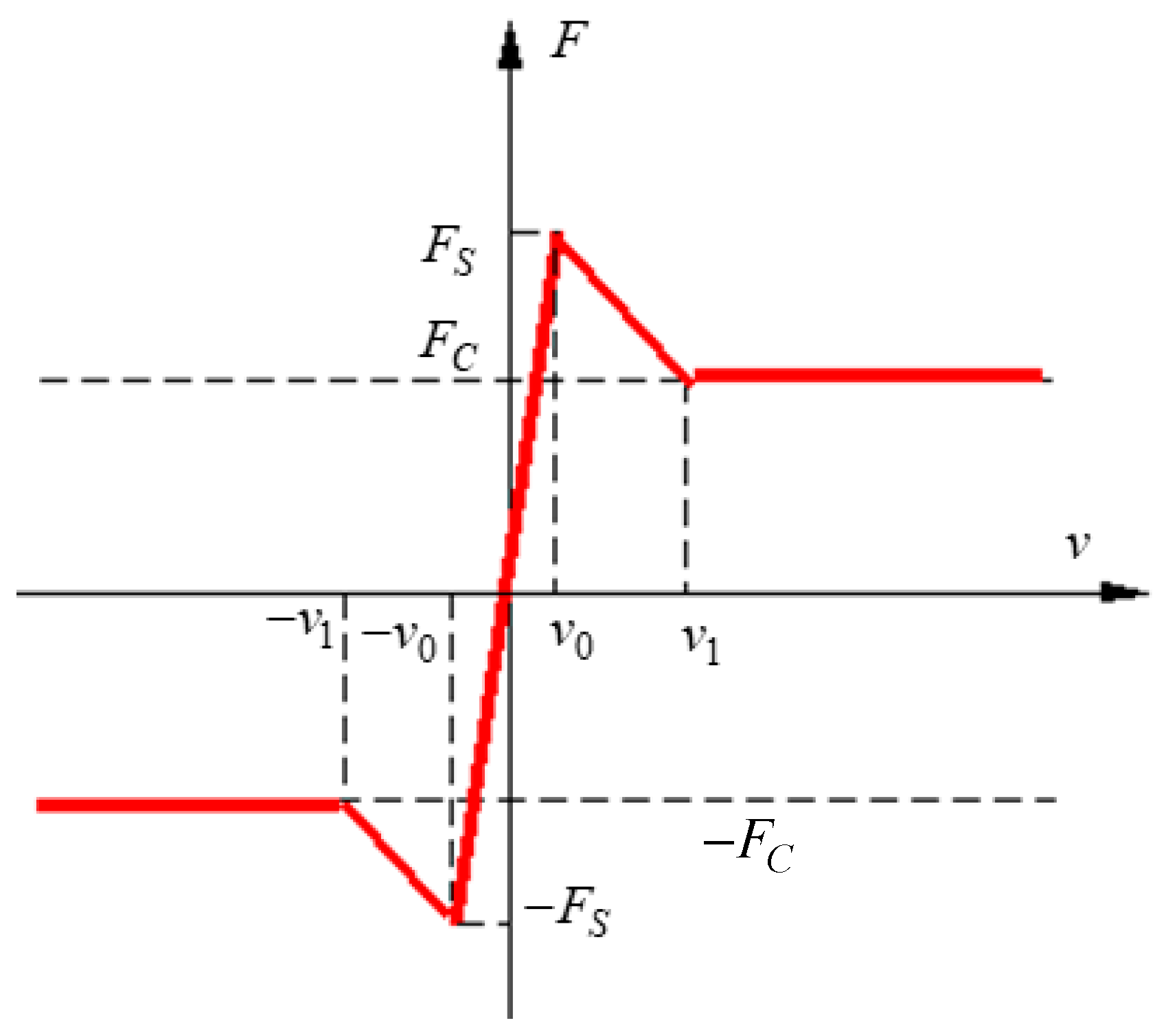
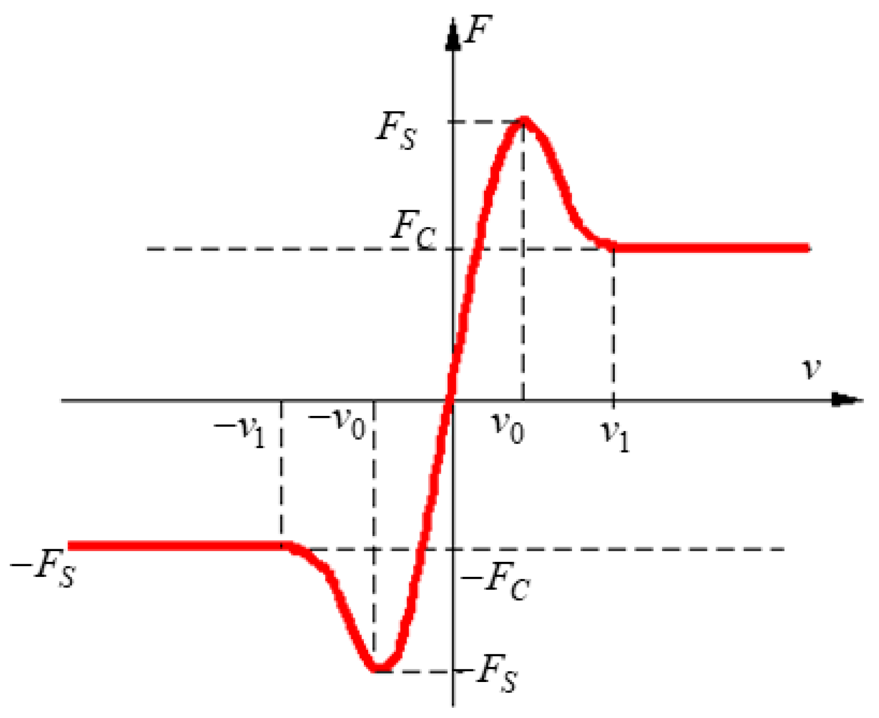
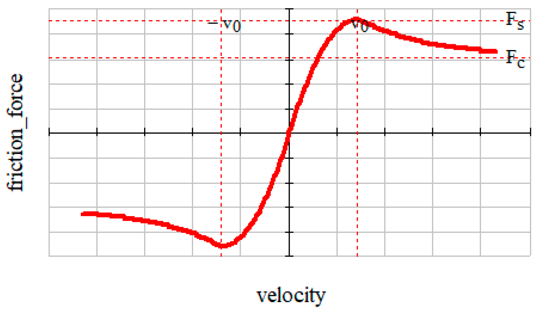
1.2. Dry Friction Models

The friction force occurs based on the interaction between the micro-asperities of boundary surfaces of the two bodies. Taylor [12] reviewed the main models that try to explain the presence of friction as a result of interactions between micro-irregularities of the contacting surfaces.

Amid the papers cited by Taylor, we are reminded of two articles, Greenwood and Williamson [13] and Greenwood and Tripp [14]. In the first [13], we are reminded that there are considered two surfaces: a smooth one and a second one, with asperities with the same radius of curvature but with differing height distributions; for two types of distributions of asperities, exponential and Gaussian, the normal force and the actual contact area are found. The hypothesis of proportionality between the normal force and the relative contact area is confirmed. In the second paper of Greenwood and Tripp [14], the research extends to the contact of the plane rough surfaces, and the normal load on the peaks of asperities is found. The conclusion reached is that for asperities that have a Gaussian peak height distribution, the actual area of contact is proportional to the load (similar to previous case). The hypothesis of a Gaussian peak height distribution for a rough surface is an ideal model. Actually, the peak distribution of asperities is quite different from the Gaussian model and, thus, the effects on the friction force are important. Considering a lubricated contact, Leighton et al. [15] highlight substantial differences between theoretical results and experimental results.

The complex phenomena involved when variable coefficients of friction are present are evidenced in the paper of Centea [16], where the torsional vibrations produced by variable dry friction coefficients from automotive clutches are analysed. The conclusion of Centea [16] is that, for the occurrence of shocks in running clutches, the sign of the gradient of the coefficient of friction with respect to velocity is definitory.

Another model, friction with stiction [17,18], is presented in Figure 3, which is similar to the Coulomb model; the difference is in the case when $v=0$, where the friction force can take any value [19] in the range $[-F_s,F_s]$, where $F_s$ is the maximum static friction, defined similarly to the Coulomb friction force as follows:

$$F_s={\mu }_s{F}_N$$

(6)

where ${\mu }_s$ is the coefficient of static friction.

The models mentioned are difficult to apply because of the following:

• The possibility of multiple values for the friction force in the case of the absence of relative motion, as Pennestri et al. [9] affirm: “In kinematic pairs with no relative motion the computation of friction forces is not straightforward”;
• The discontinuities of friction force in the vicinity of origin, where “Friction force discontinuity is a challenge for the numerical integration procedure” [9].

These mathematical difficulties increase based on the fact that the transition from static to dynamic friction is not sudden, as shown in Figure 3, but it happens in a finite time interval; this is known as the Stribeck effect [20,21].

To overcome the possibility that static friction force takes multiple values, the regularisation of the functions that describe the friction force–velocity dependency was attempted by accepting that there is a domain of velocities $[-v_0,v_0]$, symmetrical with respect to the origin, where the univalue transition from $-F_s$ to $F_s$ takes place [22,23].

To overcome the mathematical difficulties concerning the multiple values that the friction force can take in the case when the velocity between the contacting points is zero, Karnopp [24] proposes a friction model where the relative velocity is considered zero for an entire interval, and the force should be evaluated for zero velocity. The following Karnopp model eliminates the discontinuities for zero velocity and is capable of highlighting the stick–slip phenomenon as shown in Figure 4:

$$(v)=\left\{\begin{array}{c}{F}_C\left(v\right)if \left|v\right|>Dv\\ \mathit{min}(F_e,F_S\left)\mathit{sgn}(F_e\right)if \left|v\right|\le Dv\end{array}\right.$$

(7)

where $Dv$ is the half-length of the domain where $v\cong 0$ is considered, and $F\left(v\right)$ is a given function for the friction force, usually the Coulomb friction force, outside the tolerance velocity; $F_e$ is the magnitude of the resultant external force acting upon the system. In order to reduce the effect of the discontinuity at the transition from $F_s$ to $F_C$, some authors accept that this shift is not sudden, but occurs during a transition interval from $v_0$ to $v_1$, as seen in Figure 5. One can notice that the function presented in Figure 5 has slope discontinuities. A solution for smoothing the function from Figure 5, obtained by slope continuity, is shown in Figure 6.

A solution for the regularised friction force was proposed by Bengisu and Akay [25], who consider the dependency function obtained by a parabolic arch connected to an exponential arch. The analytical relation proposed in [25] for friction force is the following:

$$F(v)=\left\{\begin{array}{l}\left[-{\displaystyle \frac{F_s}{v_0^2}}(|v|-v_0{)}^2+F_s\right]sign(v),if |v|<v_0\\ \left\{F_c+\left(F_s-F_c\right)\mathit{exp}[-{\xi }_B\left(\right|v|-v_0)]\right\}sign\left(v\right),if \left|v\right|\ge v_0\end{array}\right.$$

(8)

and a plot of friction force variations is shown in Figure 7. The ${\xi }_B$ parameter is positive and represents the negative slope of the sliding state.

The mentioned models describe the friction force at a certain moment but cannot characterise phenomena such as pre-sliding displacement or frictional lag. To overcome this drawback, dynamic friction models were proposed and a first was proposed by Dahl [26,27]. The Dahl friction model assimilates the contact between the two rubbing surfaces as the contact between two brushes, one with rigid bristles and the other one with elastic bristles, which bend elastically due to relative motion; the deflection $z$, shown in Figure 8, is defined by the following differential equation:

$${\displaystyle \frac{dz}{dt}}=\left(1-{\displaystyle \frac{{\sigma }_0}{F_c}}\mathit{sgn}v\right)v$$

(9)

$$F={\sigma }_{0}z$$

(10)

where the elasticity of the bristles is given by a material characteristic denoted ${\sigma }_0$, and $F_c$ is the friction force according to the Coulomb model.

Haessig and Friedland [28] proposed a dynamic friction model that simulates the degree of random behaviour associated with the tribological conduct on the contact between two surfaces with irregularities. The model considers that the friction force is generated by the asperity deformations. Each of the contacts between asperities is modelled as the interaction between a rigid bristle and an elastic massless bristle. The contact is thus assimilated to a spring and when relative motion occurs, the deformation of the elastic bristle will generate a friction force. The vector sum of all elementary friction forces gives the total friction force.

Succeeding this, the LuGre model [29,30,31] is a generalisation of the Dahl model and is expressed by the following equation:

$${\displaystyle \frac{dz}{dt}}=\left(1-{\displaystyle \frac{{\sigma }_0}{g\left(v\right)}}z·signv\right)v+{\sigma }_{2}v$$

(11)

where the function $g\left(v\right)$ is given by the following:

$$g\left(v\right)=F_c+(F_s-F_c)\mathit{exp}[-\left(\right|v|/v_s{)}^2]$$

(12)

and the friction force has the following expression:

$$F={\sigma }_{0}z+{\sigma }_1{\displaystyle \frac{dz}{dt}}+{\sigma }_{2}v$$

(13)

Similar to the Dahl model, ${\sigma }_0$ characterises the compliance of the bristle; ${\sigma }_1$ describes the contact damping of the bristle and ${\sigma }_2$ characterises the viscous damping; and $v_s$ is the velocity characteristic to Stribeck friction.

1.3. Choosing the Friction Model

From the models briefly presented above, one can affirm that when the problem of modelling a dynamic system arises, multiple friction models can be considered as options. No matter the chosen model, whether a simpler or more complex one, the final goal is to obtain a model that is capable of characterising the physical reality as genuinely as possible.

A simple model has as a disadvantage the difficult folding on the physical reality but presents the advantage of requiring fewer parameters, which can be precisely found. A complex model is helpful because it is more flexible but presents the drawback of a larger number of parameters necessary to be stipulated. To sustain this affirmation, we cite Pennestri et al. [9], who state, with reference to the Dahl model, ”The authors could not find a table relating the Coulomb friction coefficients with Dahl friction parameters”; next, they indicate two reference sources where the manner of obtaining the tribological parameters required by dynamic models are specified [32,33]. Another study concerning these parameters is from Arnoux et al. [34]. A more complex model accepts that the displacement of the mobile body consists of an elastic component and a plastic component [35,36].

In our study, four friction force models were considered—the Coulomb, Coulomb friction with stiction, Dahl, and LuGre—for modelling the evolution of the system from Figure 1. The values of the parameters required by the specified models are as discussed in [3]. The mass of the mobile body (denoted 1) is $\mathrm{m}=1 \mathrm{k}\mathrm{g}$, the velocity of the belt $v_b=0.1 \mathrm{m}/\mathrm{s}$, the spring stiffness $k_e=2 \mathrm{N}/\mathrm{m}$, the coefficient of static friction ${\mu }_s=0.15$, the coefficient of dynamic friction ${\mu }_d=0.1$, the transition velocity $v_0=0.001 \mathrm{m}/\mathrm{s}$, the shape factor $\xi =\mathrm{s}/\mathrm{m}$, the stiffness coefficient ${\sigma }_0=10^{5 }\mathrm{N}/\mathrm{m}$, the damping coefficient ${\sigma }_1=\sqrt{10^5} \mathrm{N}·\mathrm{s}/\mathrm{m}$, and the viscosity coefficient ${\sigma }_2=0.1 \mathrm{N}·\mathrm{s}/\mathrm{m}$.

In most of the papers that consider dry friction, when the relative velocity exceeds a certain value (the transition velocity $v_0$) the coefficient of friction becomes constant and equal to the kinetic friction coefficient. In our case, the kinetic coefficient of friction presents periodical jumps and, additionally, the presence of two contacts may lead to many situations: the same kinetic coefficient of friction in both contacts, different values in the two contacts, or a contact with stiction and the other with sliding.

The equations of motion were integrated using Mathcad 14 software, applying the Runge–Kutta 4 formula [37,38] with constant step under the assumption that the body is initially at rest at the origin. The plots of the displacement are presented in Figure 9, and the variations of velocity are shown in Figure 10, comparatively, for the four friction models. The comparison of the friction forces for the four models is presented in Figure 11. Details from Figure 11 are presented in Figure 12, concerning friction force variations immediately after the start of motion.

From Figure 9 and Figure 10 it can be noticed that, considering kinematical aspects, there is significant similarity between the Coulomb and Dahl models on one side and similarity between the Coulomb with stiction model and the LuGre model on the other side. Regarding the friction force, Figure 11 reveals major differences among all of the considered models. From Figure 12, it can be remarked that these variances are more pronounced immediately after the start of motion. It should be mentioned that the graphs obtained for the Dahl and LuGre models are identical to the ones from the article of Marques et al. [3], confirming the correctness of the models and the methodology of numerical integration.

The main goal of the paper is to provide a theoretical model capable of describing the motion of a mobile body with one degree of freedom, (1DOF), which executes planar motion in a vertical plane and has two Hertzian contact points with dry friction where the coefficient of friction varies over regions. In our research, we obtained an analytical expression for the time variation of the friction forces from the two contacts. The analysis of the friction models from the literature for the classical problem of an oscillatory system composed of a mass, spring, and mobile horizontal belt evidenced that the envisaged motion is framed in two large classes. In the present paper, models were chosen for the law of motion corresponding to friction from the two classes; to be specific, the Coulomb with stiction model and the Bengisu–Akay model were the options. For these two friction models, the equations of motion were integrated and, by convenient selection of geometrical, kinematical, and tribological parameters, the three important cases of motion that may occur were highlighted:

• Oscillatory motion;
• Revolving motion;
• Motion with disruption of the upper contact.

This paper opens a perspective for future research; the main research consists of experimentally validating the proposed model. In this paper, we obtained the law of time variation of the friction forces that act on the two contacts.

2. Materials and Methods

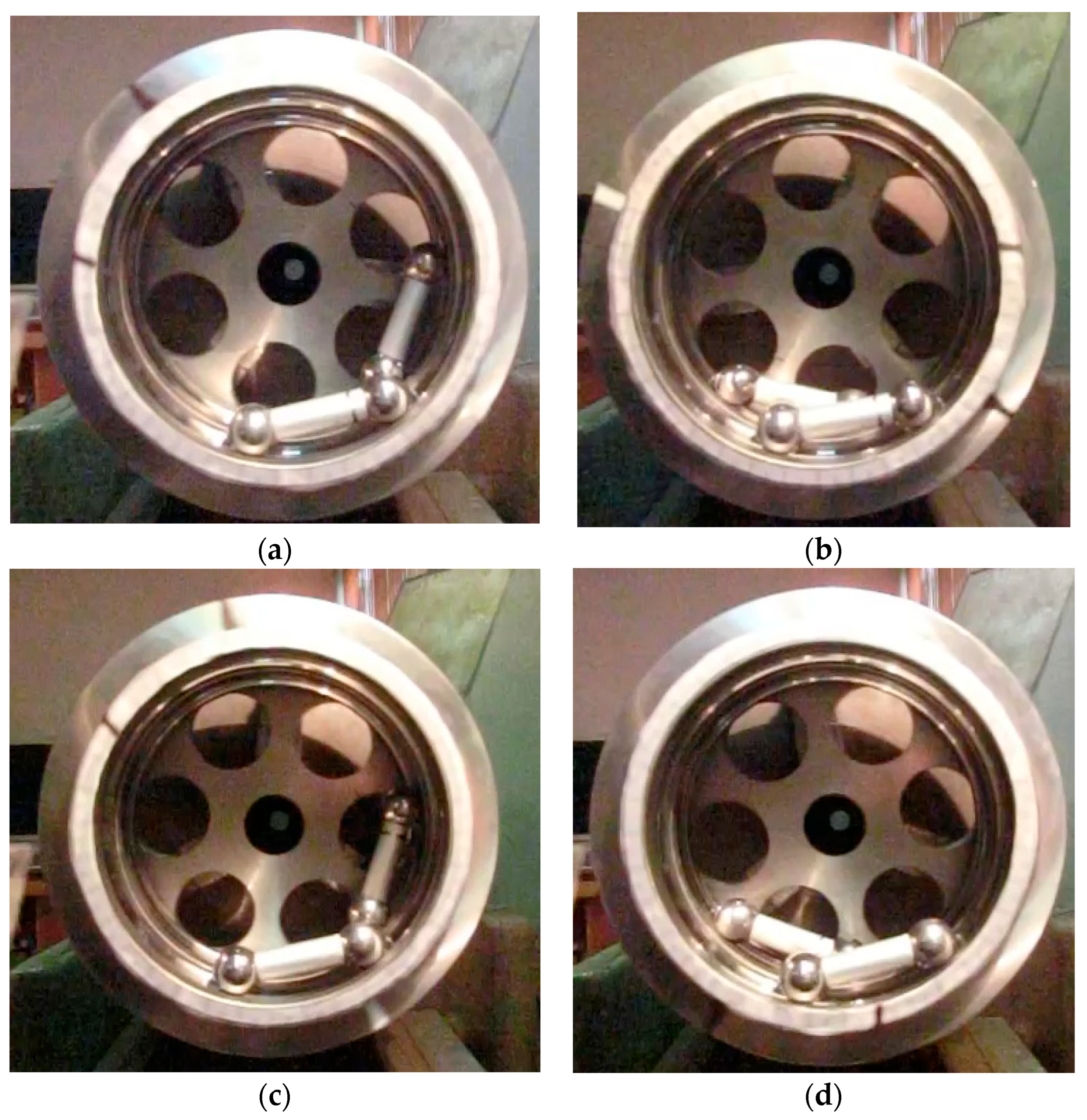
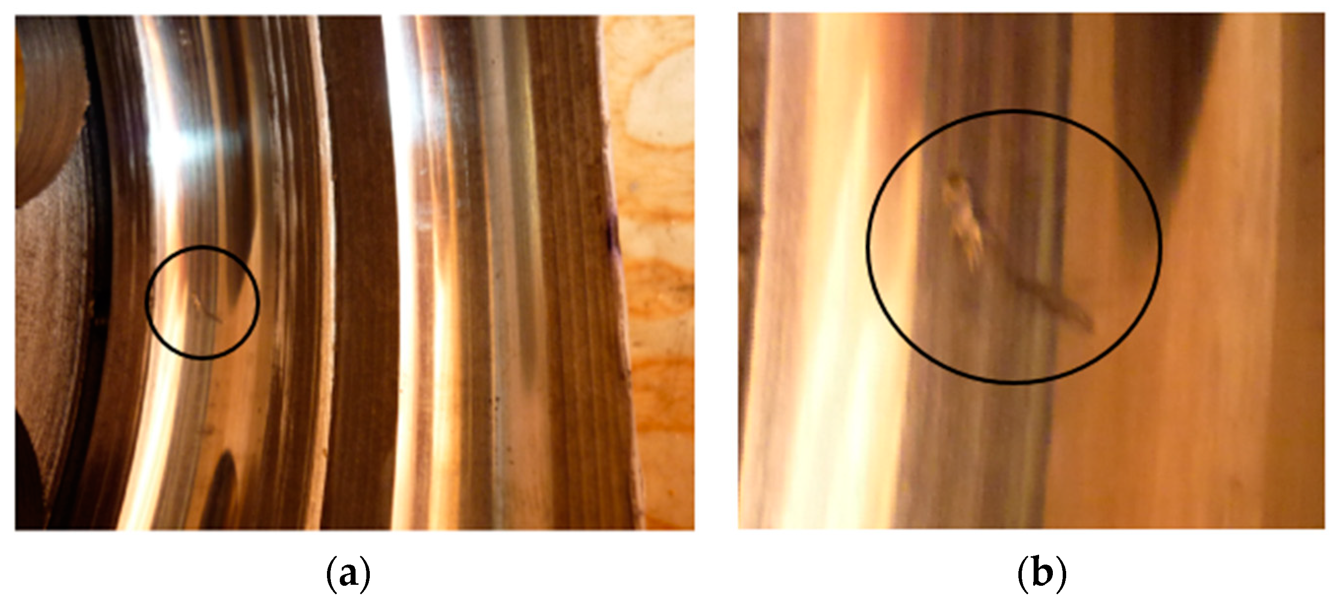
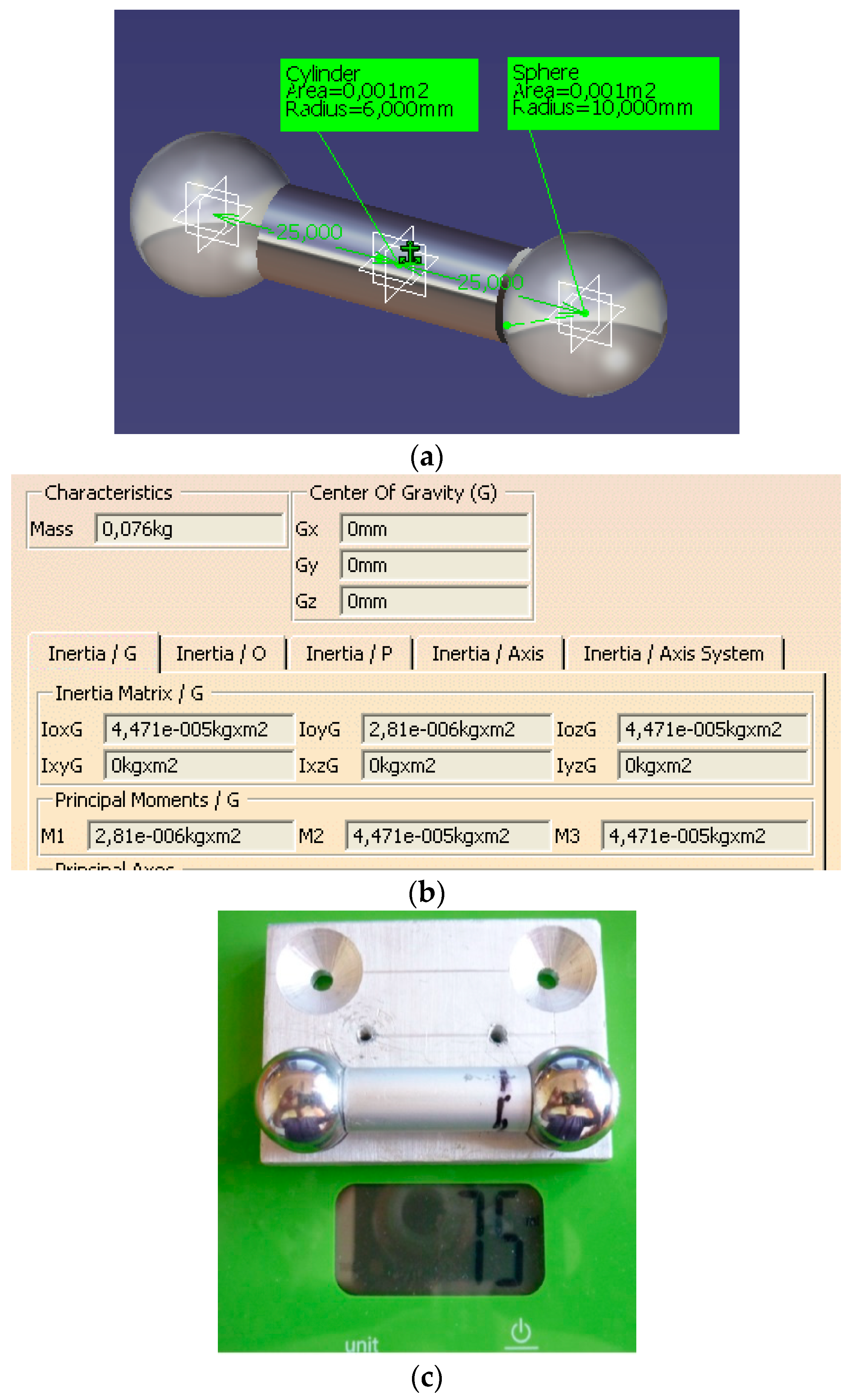
2.1. Experimental Evidence

We aimed to experimentally highlight the qualitative aspects of the effects of dry friction in dynamic systems. Our research started from the observation that two forces act in the dynamic system from Figure 1: the conservative force, represented by the elastic force $F_e$ generated by the elastic element of the helical spring, and the dissipative force, represented by the friction force $F_f$. The elastic force is considered rigorously proportional to the deformation of the spring. In fact, this aspect is difficult to obtain due to the non-linearities occurring in the coupling regions of the spring with the ground and with the mobile body, and due to the internal friction from the material of the spring, this actually being a Kelvin–Voigt body [39]. All these non-linearities will remove the dynamic model obtained under the hypothesis of elastic force–spring deformation proportionality from the accurate evolution of the actual system. For this reason, we proposed that the effect of dry friction be analysed based on the system from Figure 13 instead of the dynamic system from Figure 1. The new system consists of a circular ring of radius $R$ that rotates about a horizontal axis with the known angular velocity $\omega \left(t\right)$. Inside the ring, a small body that contacts the ring at a unique point is placed. Assuming that the relative velocity of the contact point from the body is oriented as shown in Figure 13, the next forces can be identified as acting upon the body: the body weight $\mathit{G}$ with its components (normal ${\mathit{G}}_n$ and tangential ${\mathit{G}}_t$) and the following reactions: the normal reaction $N$ and the tangential reaction (or the friction force)${\mathit{F}}_f$.

The advantage of the new system consists of the fact that part of the conservative force is now played by the tangential component of body weight, and it does not depend on the elastic properties of the materials from which the mobile body and the ring are made.

To materialise the ring, the idea of an outer ball bearing ring [40] was employed. The uncontrolled rotations of the body must be avoided; thus, starting from the solution of two rigidly attached balls, we built the mobile body by firmly connecting two identical ball bearings by an aluminium rod. The co-axiality between the rod axis and the centre line was ensured by making two conical holes at the ends of the rod that are co-axial to the rod axis; this ensures the self-laying of the balls with their centres on the axis of the rod, Figure 14.

When the mobile body is placed with both balls on the rolling race of the outer bearing ring, it was certified that the motion of the axis of the mobile body is in the vertical plane. This is a second advantage compared to the system from Figure 1, where the risk exists of a motion occurring in the normal direction to the plane of the sketch. The necessity of obtaining qualitative results compels that the system does not perform uncontrolled motions. Therefore, there is imposed cancellation of the rotational motion with respect to system’s own axis. For this purpose, two identical outer ball bearing rings 1 were used, assembled on a special designed part 2, as shown in Figure 15. Part 2 has an outer cylindrical region (a), accurately constrained coaxially with respect to the inner cylindrical surface on which the bearing rings are centred. via this surface, the entire assembly is mounted on the machine tool mandrel used for driving. One can notice that angular scale 3 with divisions was attached to this part in order to stipulate the position of the mobile body with respect to the rings.

The problem of blocking rotational motion arose. Initially, the solution used two mobile identical bodies attached to an aluminium plate where conical holes self-positioned the balls, as shown in Figure 16a. It was observed that after positioning the balls into the conical holes, the rods were not necessary, so the final solution for the oscillating body is the one presented in Figure 16b.

The design of the device is presented in Figure 17a and the actual device from the lab is shown in Figure 17b. One can see that on the mounting plate was attached pointer 1, needed for stipulating the position of the body with respect to the driving part. On the plate, acceleration sensor 2 was also attached by two screws.

The device was mounted on the universal lathe chuck in order to drive it into motion with controlled angular velocity, as shown in Figure 18a. In the first stage, the motion was studied via optical methods. The motion of the body was video captured with a high-speed camera (240 frames/s), and then analysed by splitting into frames using QuickTime 7.7.9 software. It was noticed that the mobile body performs an oscillatory motion. Then, using an angular scale, the position of the body at the end of race (maximum amplitude) was precisely identified and, therefore, the absolute motion of the body was found.

The variations with time of the angular amplitude are presented in Figure 19.

We aimed to validate the theoretical model through experiments using the oscillatory body, on top of which an acceleration sensor was placed in order to describe the actual motion of the body. The body, which makes four contacts, two with each ring, is a statically undetermined system. From the four contact points, only three may be simultaneously coplanar. When the contact between the body and the race moves into different positions, there are occurring micro-shocks that perturbate the geometry of the loading and implicitly alter the law of motion of the body. For this reason, we chose the mobile body consisting of two balls and a rod, making two contacts with the same ring. Accepting that during the motion the mobile body does not have rotation about the axis of the centres of the balls, the obtained dynamic system becomes statically determined. The drawback of this solution is the impossibility of placing a sensor on the body.

In Figure 20 there are images showing two identical mobile bodies and two coaxial bearing rings. A mobile body is obtained by connecting two balls with a cylindrical rod; each body is placed on the race of a ring. It was noticed that the motions of the two bodies differ, though, in theory, they should be identical. By reversing the two bodies, it was noted that the body contacting the rear ring has a broader motion than the body from the front ring. Surface analysis of the rings’ races revealed a scratch Figure 21a and a detail of the scratch Figure 21b on the race of the rear ring. The surface of the scratch is much rougher than the rest of the race, thus when the scratch contacts a ball, the friction force presents a sudden increase and acts as external excitation.

2.2. Proposed Mathematical Model

The dynamic model of the system from Figure 20 is presented in Figure 22. The mobile body consists of two identical spheres of radius $r$ rigidly connected by rods, and the distance between the centres of the spheres is $O_1{O}_2=2a$.

The mobile body is characterised by its mass $M$ and its axial moment of inertia with respect to a centric axis normal to the plane of motion $J_{\Gamma z}$. The mobile ring of radius $R$ has the motion stipulated with respect to $OX$ by the angle $\theta$ between the vector radius of the centre of mass $\Gamma$ and the $OX$ axis. Two regions are identified on the inner surface of the ring: a region of angular opening $2\Delta \theta$ characterised by ${{\mu }^{\prime }}_s$, the coefficient of static friction and ${{\mu }^{\prime }}_k$ the coefficient of dynamic friction, and the second region, complementary, characterised by ${{\mu }^{″}}_s$ and ${{\mu }^{″}}_k$. The mobile body and the ring have two points of contact, $C_1$ and $C_2$. The versors ${\mathit{n}}_{1,2}$ and ${\mathit{t}}_{1,2}$ are defined in these contact points, and have radial and tangential directions (with respect to the ring), respectively, as shown in Figure 22. The system of vectors $\mathit{i}$, $\mathit{j}$ attached to the mobile body is defined: the versor $\mathit{i}$ has the $O\Gamma$ direction and the versor $\mathit{j}$ is normal to $\mathit{i}$ and rotated in a trigonometrical direction.

The forces acting upon the mobile body are the gravity $\mathit{G}$ applied at the centre of mass $\Gamma$ and the reactions from the contact points $C_1$ and $C_2$: the normal reactions ${\mathit{N}}_1,{\mathit{N}}_2$ directed in radial directions and the friction forces ${\mathit{F}}_{f_1}$, ${\mathit{F}}_{f_2}$ tangent to the circumference of the ring. In order to model the friction forces, two models from the four presented in the Introduction section were adopted: the Coulomb model and the Bengisu–Akay model, according to the relations 6–8, for which the friction forces are proportional to the normal forces. The Bengisu–Akay model was chosen because, according to Equation (8), the magnitudes of the friction forces, both static and dynamic, are proportional to the normal force. For the LuGre model (Equations (11)–(13)), this is not valid and therefore, the integration of the equation of motion is very intricate.

The theorem of the motion of the centre of mass and the moment of momentum theorem with respect to the centre of mass $\Gamma$ [6] are applied, in order to establish the motion of the body.

The theorem of the motion of the centre of mass is as follows:

$$M{\mathit{a}}_{\Gamma }=\mathit{G}+{\mathit{N}}_1+{\mathit{N}}_2+{\mathit{T}}_1+{\mathit{T}}_2$$

(14)

The moment of momentum theorem is the following:

$$M(-\xi {\dot{\phi }}^2\mathit{i}+\xi \ddot{\phi }\mathit{j})=Mg\mathit{I}-N_1{\mathit{n}}_1-N_2{\mathit{n}}_2+K_1{N}_1{\mathit{t}}_1+K_2{N}_2{\mathit{t}}_2$$

(15)

In Equation (15), $\xi$ represents the distance from the origin $O$ to the centre of mass $\Gamma$, and $K_{1,2}$ are constants of proportionality to be stipulated next. The vectors from Equation (14) will be expressed as functions of the versors $\mathit{i},\mathit{j}$, and it results in a system with unknowns in the law of motion $\phi \left(t\right)$ and in the magnitudes of the normal reactions.

$$\left[\begin{array}{c}-M\xi {\dot{\phi }}^2\\ -M\xi \ddot{\phi }\end{array}\right]=\left[\begin{array}{c}Mg\mathit{cos}\phi \\ -Mg\mathit{sin}\phi \end{array}\right]+\left[\begin{array}{c}-N_1\mathit{cos}\beta \\ N_1\mathit{sin}\beta \end{array}\right]+\left[\begin{array}{c}-N_2\mathit{cos}\beta \\ -N_2\mathit{sin}\beta \end{array}\right]+\left[\begin{array}{c}{K}_1{N}_1\mathit{sin}\beta \\ K_1{N}_1\mathit{cos}\beta \end{array}\right]+\left[\begin{array}{c}-K_2{N}_2\mathit{sin}\beta \\ K_2{N}_2\mathit{cos}\beta \end{array}\right]$$

(16)

The system of Equation (16) is solved and the magnitudes of the normal reactions are found:

$$\left\{\begin{array}{l}{N}_1=M{\displaystyle \frac{[\xi \ddot{\phi }\mathit{sin}\beta -\xi {\dot{\phi }}^2\mathit{cos}\beta -g\mathit{cos}(\phi +\beta )]K_2+[\xi \ddot{\phi }\mathit{cos}\beta +\xi {\dot{\phi }}^2\mathit{sin}\beta +g\mathit{sin}(\phi +\beta \left)\right]}{(K_1-K_2)\mathit{cos}2\beta +(K_1{K}_2+1)\mathit{sin}2\beta }}\\ N_2=M{\displaystyle \frac{[\xi \ddot{\phi }\mathit{sin}\beta +\xi {\dot{\phi }}^2\mathit{cos}\beta +g\mathit{cos}(\phi -\beta )]K_2+[-\xi \ddot{\phi }\mathit{cos}\beta +\xi {\dot{\phi }}^2\mathit{sin}\beta -g\mathit{sin}(\phi -\beta \left)\right]}{(K_1-K_2)\mathit{cos}2\beta +(K_1{K}_2+1)\mathit{sin}2\beta }}\end{array}\right.$$

(17)

Next, the moment of momentum theorem is applied with respect to an axis passing through the centre of mass:

$$J_{\Gamma z}{\ddot{\phi }}_2\mathit{k}=\overline{\Gamma C_1}\times (-N_1{\mathit{n}}_1+K_1{N}_1{\mathit{t}}_1)+\overline{\Gamma C2}\times (-N_2{\mathit{n}}_2+K_2{N}_2{\mathit{t}}_2)$$

(18)

The vectors from Equation (18) are written in the function of the versors $\mathit{i}$ and $\mathit{j}$ and the following results:

$$\left[\begin{array}{c}0\\ 0\\ J_{{\Gamma }_z}\ddot{\phi }\end{array}\right]=\left\{\left[\begin{array}{c}-\xi \\ 0\\ 0\end{array}\right]+\left[\begin{array}{c}R\mathit{cos}\beta \\ -R\mathit{sin}\beta \\ 0\end{array}\right]\right\}\times \left\{\left[\begin{array}{c}-N_1\mathit{cos}\beta \\ N_1\mathit{sin}\beta \\ 0\end{array}\right]+\left[\begin{array}{c}{K}_1{N}_1\mathit{sin}\beta \\ K_1{N}_1\mathit{cos}\beta \\ 0\end{array}\right]\right\}+\left\{\left[\begin{array}{c}-\xi \\ 0\\ 0\end{array}\right]+\left[\begin{array}{c}R\mathit{cos}\beta \\ R\mathit{sin}\beta \\ 0\end{array}\right]\right\}\times \left\{\left[\begin{array}{c}-N_2\mathit{cos}\beta \\ -N_2\mathit{sin}\beta \\ 0\end{array}\right]+\left[\begin{array}{c}-K_2{N}_2\mathit{sin}\beta \\ K_2{N}_2\mathit{cos}\beta \\ 0\end{array}\right]\right\}$$

(19)

From the above equation, we can obtain the following:

$$J_{\Gamma z}=\left[K_1\right(R-\xi \mathit{cos}\beta )-\xi \mathit{sin}\beta ]N_1+\left[K_2\right(R-\xi \mathit{cos}\beta )+\xi \mathit{sin}\beta ]N_2$$

(20)

Replacing in Equation (19) the expression of normal reactions (17), the differential equation of motion of the mobile body is obtained as follows:

$$\ddot{\phi }={\displaystyle \frac{B}{A}}$$

(21)

where

$$\begin{array}{l}A=J_{{\Gamma }_z}+M\xi {\displaystyle \frac{\left[K_1\left(\xi \mathit{cos}\beta -R\right)+\xi \mathit{sin}\beta \right]\left(K_2\mathit{sin}\beta +\mathit{cos}\beta \right)+\left[K2\right(\xi \mathit{cos}\beta -R)-\xi \mathit{sin}\beta ](K_1\mathit{sin}\beta -\mathit{cos}\beta )}{(K_1-K_2)\mathit{cos}2\beta +(K_1{K}_2+1)\mathit{sin}2\beta }}\\ B=M{\displaystyle \frac{\left[\begin{array}{c}\{\xi {\dot{\theta }}^2\mathit{sin}\beta +g\mathit{sin}(\phi +\beta )-K_2[\mathit{cos}(\phi +\beta )g+\xi {\dot{\phi }}^2\mathit{cos}\beta \left]\right\}\left[K_1\right(\xi \mathit{cos}\beta -R)+\xi \mathit{sin}\beta ]+\\ \{\xi {\dot{\phi }}^2\mathit{sin}\beta +g\mathit{sin}(\phi -\beta )-K_1[\mathit{cos}(\phi -\beta )g+\xi {\dot{\phi }}^2\mathit{cos}\beta \left]\right\}\left[K_2\right(\xi \mathit{cos}\beta -R)-\xi \mathit{sin}\beta ]\end{array}\right]}{(K_1-K_2)\mathit{cos}2\beta +(K_1{K}_2+1)\mathit{sin}2\beta }}\end{array}$$

(22)

The coefficients of friction required by the Bengisu–Akay model are the following for the first domain:

$${\mu }^{\prime }(v)=\left\{\begin{array}{l}{{\mu }^{\prime }}_s\left[1-{\left(1-{\displaystyle \frac{\left|v\right|}{v}}\right)}^2\right]\mathit{sgn}v,if |v|\le v_0\\ {{\mu }^{\prime }}_k\left[1+\left({\displaystyle \frac{\left|v\right|}{v}}\right)\mathit{exp}[-\alpha (|v|-v_0)\right]\mathit{sgn}v,if |v|\le v_0\end{array}\right.$$

(23)

For the second domain, the coefficients are the following:

$${\mu }^{″}(v)=\left\{\begin{array}{l}{{\mu }^{″}}_s\left[1-{\left(1-{\displaystyle \frac{\left|v\right|}{v}}\right)}^2\right],if |v|\le v_0\\ {{\mu }^{″}}_k\left[1+\left({\displaystyle \frac{\left|v\right|}{v}}\right)\mathit{exp}[-\alpha (|v|-v_0)\right]\mathit{sgn}v,if |v|\le v_0\end{array}\right.$$

(24)

Concerning the Coulomb model, the coefficients of friction are expressed as follows:

$${\mu }^{\prime }\left(v\right)={{\mu }^{\prime }}_k\mathit{sgn}v$$

(25)

and, respectively,

$${\mu }^{″}\left(v\right)={{\mu }^{″}}_k\mathit{sgn}v$$

(26)

An extremely important problem exists identifying the coefficient of friction from the contact points $C_1$ and $C_2$ at a certain time. This difficulty arises from the fact that both the ring and the body may take the same position at different moments, but the two angles of position differ by a multiple of $2\pi$.

$$F_{f_{1,2}}=\left\{\begin{array}{c}{\mu }^{\prime }{N}_{1,2}, if C_{1,2}\in arc\left(P_1{P}_2\right)\\ {\mu }^{″}{N}_{1,2}, if C_{1,2}\notin arc\left(P_1{P}_2\right)\end{array}\right.$$

(27)

In order to operate with relation (27), the decision $C_{1,2}\in arc\left(P_1{P}_2\right)$ or $C_{1,2}\notin arc\left(P_1{P}_2\right)$ is required, according the kinematical parameters of the model. Specifically, for all angles involved, the multiples of $2\pi$ should be eliminated and thus, for the position angle, it results in a value within a domain of length $2\pi$. To these ends, the following function is defined:

$$\psi \left(x\right)=x-2\pi floor(x/2\pi )$$

(28)

where $floor\left(x\right)$ is the function that returns the greatest integer smaller than $x$. The function $floor\left(x\right)$ can be found as predefined in the libraries of usual software such as Mathcad14 [41] and MATLAB2007 [42]. In Figure 23, it can be noticed that the function $\psi \left(x\right)$ provides values in the domain $\left[0,2\pi \right).$

The analysis is substantially condensed if the reference system is chosen to be attached to the ring. The reference straight line for angle measurements is the line passing through the point $P_1$. The position angles of the two points of contact in the system fixed to the ring are the following:

$$\left\{\begin{array}{c}\angle P_{1}O{C}_1=\phi -\theta +\Delta \theta -\beta \\ \angle P_{1}O{C}_2=\phi -\theta +\Delta \theta +\beta \end{array}\right.$$

(29)

Applying these position angles, the final forms of the coefficients $K_1$ and $K_2$ are the following:

$$K_1=\left\{\begin{array}{l}-{\mu }^{\prime }\left[\right(\dot{\phi }-\dot{\theta }\left)R\right], if 0\le \psi (\phi -\theta +\Delta \theta -\beta )<2\Delta \\ -{\mu }^{″}\left[\right(\dot{\phi }-\dot{\theta }\left)R\right], if 2\Delta \le \psi (\phi -\theta +\Delta \theta -\beta )<2\pi \end{array}\right.$$

(30)

$$K_2=\left\{\begin{array}{l}-{\mu }^{\prime }\left[\right(\dot{\phi }-\dot{\theta }\left)R\right], if 0\le \psi (\phi -\theta +\Delta \theta +\beta )<2\Delta \\ -{\mu }^{″}\left[\right(\dot{\phi }-\dot{\theta }\left)R\right], if 2\Delta \le \psi (\phi -\theta +\Delta \theta +\beta )<2\pi \end{array}\right.$$

(31)

One can be noticed that, using Equations (22)–(24) and (29)–(31), the equation of motion (22) has a strong non-linear character and for solving it, a numerical integration method is mandatory. After integration using the Runge–Kutta 4 formula with constant step method, the law of motion is obtained. Next, the law of variation of the normal reactions from the contact points $C_1$, $C_2$, according to relation (17), is necessary. This is essential because the constraints from the two contacts are unilateral, [5] and all the obtained relations are valid for the following:

$$\left\{\begin{array}{c}{N}_1>0\\ N_2>0\end{array}\right.$$

(32)

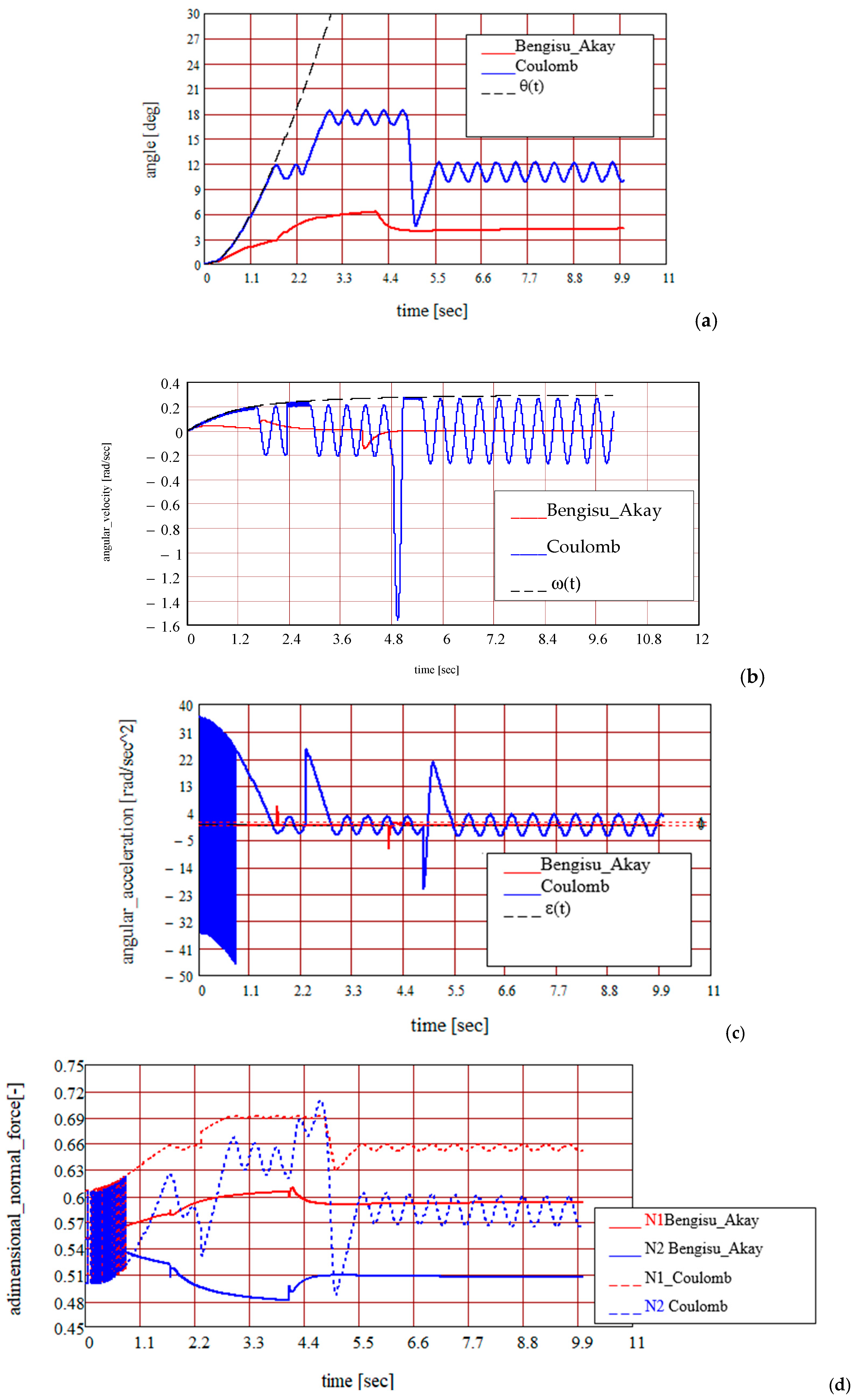
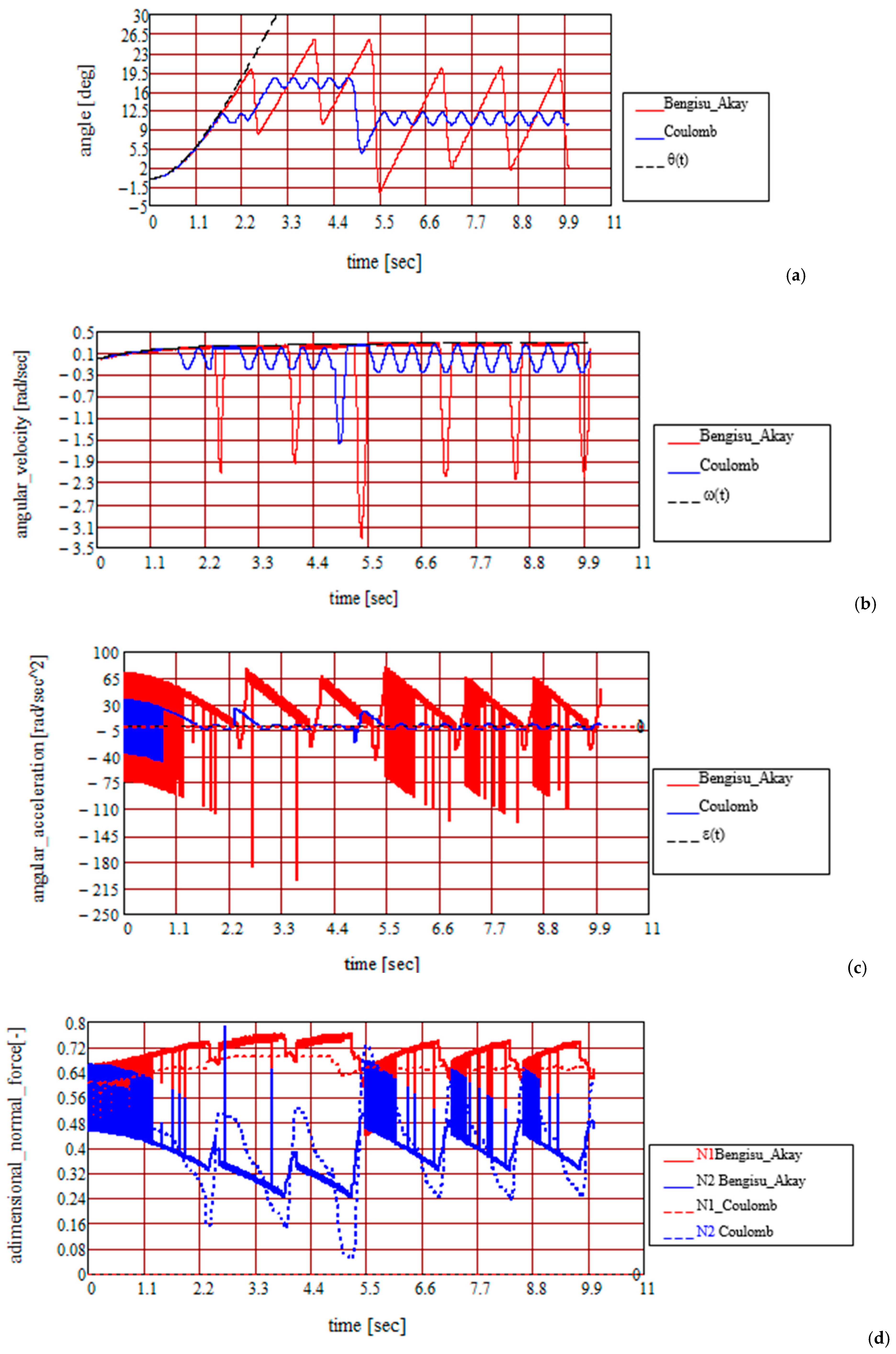
3. Results and Discussion

In order to validate the theoretical results obtained for the law of motion of the body and the reactions, the body shown in Figure 20 was chosen as an oscillatory system. It consists of two spheres of $10 \mathrm{m}\mathrm{m}$ diameter attached firmly to an aluminium cylindrical rod into the conical holes from the ends of the rod. The distance between the centres of the balls is $2a=50 \mathrm{m}\mathrm{m}$, and it is important for finding the angle $2\beta$, shown in Figure 22.

$$2\beta =\mathit{asin}[a/(R-r)]={48.504}^{\circ }$$

(33)

The body was modelled in CATIA.V5R17 as an assembly [43], shown in Figure 24a, with the inertial characteristics, the mass $M$, and the central moment of inertia $J_{\Gamma z}$. The values obtained, $M=0.076\mathrm{kg}$ and $J_{\Gamma z}=4.47\times 10^{-5} \mathrm{kg}·{\mathrm{m}}^2$, can be seen in the captures from Figure 24b. The mass of the actual body was measured on a scale, as shown in Figure 24c.

In Figure 25, Figure 26, Figure 27 and Figure 28, the results obtained are presented for different values of the parameters $\alpha$ and $v_0$ of the Bengisu–Akay model, with all other parameters kept constant. The law of motion of the ring, $\theta \left(t\right)$ was chosen as the following:

$$\theta \left(t\right)={\Phi }_0[t·\mathit{atan}t-0.5\mathit{ln}(1+t^2)]$$

(34)

and ensuring an angular velocity of the following:

$$\omega \left(t\right)={\Theta }_0·\mathit{atan}t$$

(35)

The angular velocity is continuous in origin and, with time, tends asymptotically to a constant value. Note that for large values of $\alpha$ and small values of $v_0$, the results of the two models are identical, as shown in Figure 28. Therefore, in the next Figure 29, Figure 30, Figure 31, Figure 32 and Figure 33 this situation is considered, and there are presented only the variations in the angular velocity and in the normal reactions from the contact points. Depending on the geometric characteristics of the dynamic system and of the tribological parameters, the oscillatory body may perform oscillatory motion, rotatory motion, or the contact $C_2$ may interrupt and the actual equations are no longer valid. To decide which of these situations corresponds to a given case, both kinematic parameters (position, angular velocity, etc.) and dynamic parameters (magnitudes of normal reactions) must be observed. For example, in Figure 30a, the evolution of angular velocity of the oscillatory body is shown (red line), as well as the excitatory angular velocity of the ring. In Figure 30b, variations in the magnitude of normal reactions in the contact points $C_1$ (red line) and $C_2$ (blue line) are presented. The body exhibits oscillatory motion as the angular velocity presents a change in sign. There is a certain moment when the normal reaction $N_2=0$; that is, the upper contact disrupts.

The case of a dynamic system that undergoes rotational motion with separation is presented in Figure 33. The rotational character of the motion is justified by the plot of $\varphi \left(t\right)\Phi \left[\right(N_2\left(t\right)]$. In Figure 33c, where $\varphi \left(t\right)$ is the rotation angle of the vector radius of the centre of mass $\Gamma$, $N_2$ is the magnitude of the normal reaction from point $C_2$, and $\Phi \left(x\right)$ is the Heaviside step function.

$$\Phi (x)=\left\{\begin{array}{c}1,if x\ge 0\\ 0,if x<0\end{array}\right.$$

(36)

The graphical depiction confirms that the rotation angle presents continuous increase for the first 0.2 s from launching and separation from contact point $C_2$ occurs. During this interval, the angle $\varphi$ increases continuously until a value of $9rad>2\pi rad$, corresponding to the separation time. One can conclude that during the interval from launching to separation, more than a complete rotation was made; thus, the rotational character of the motion is justified.

The model is not universally valid but it can be adapted for other systems:

• Geometries (ring radius R, balls radius r, distance between the centres of the balls a;
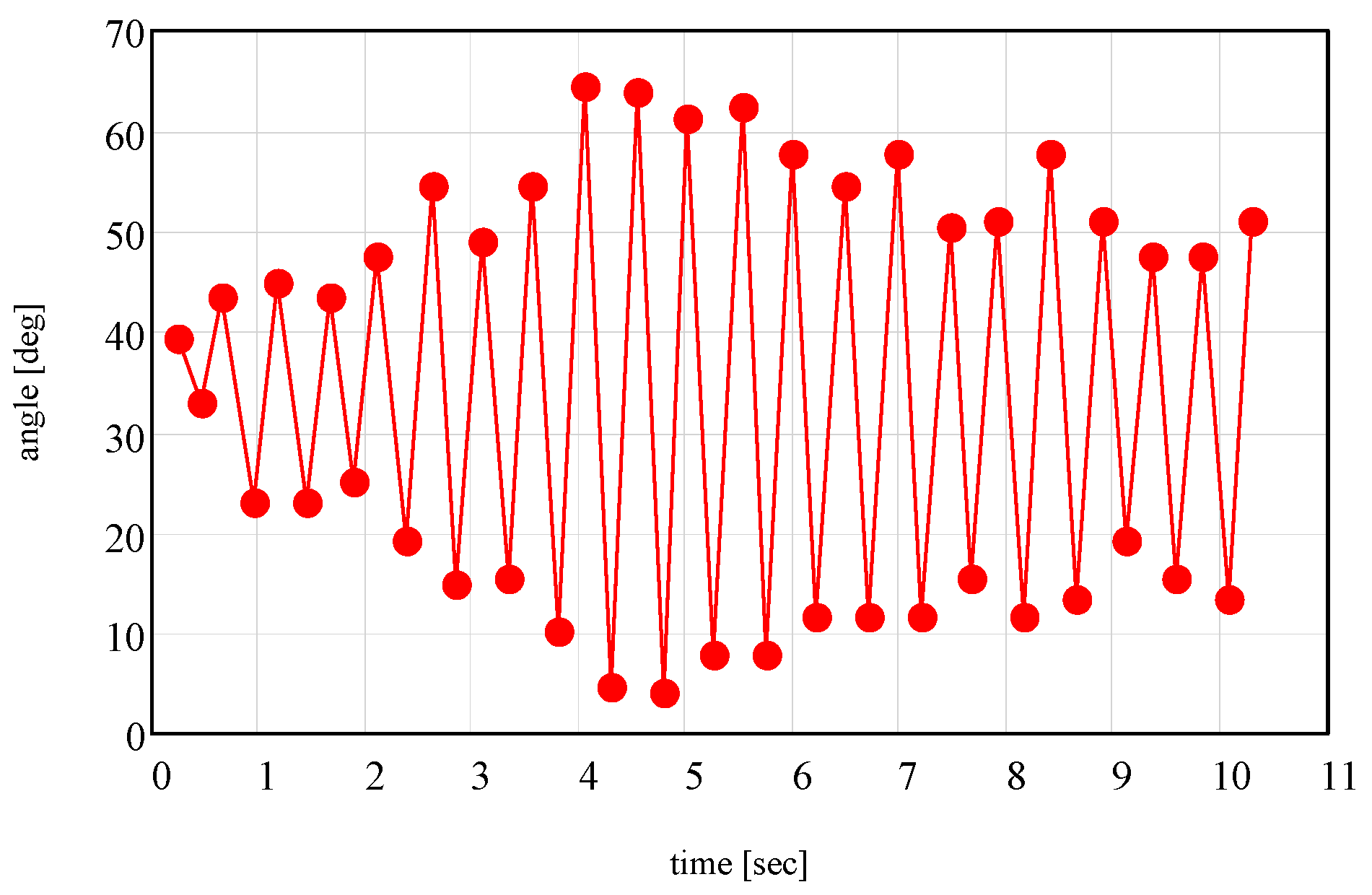
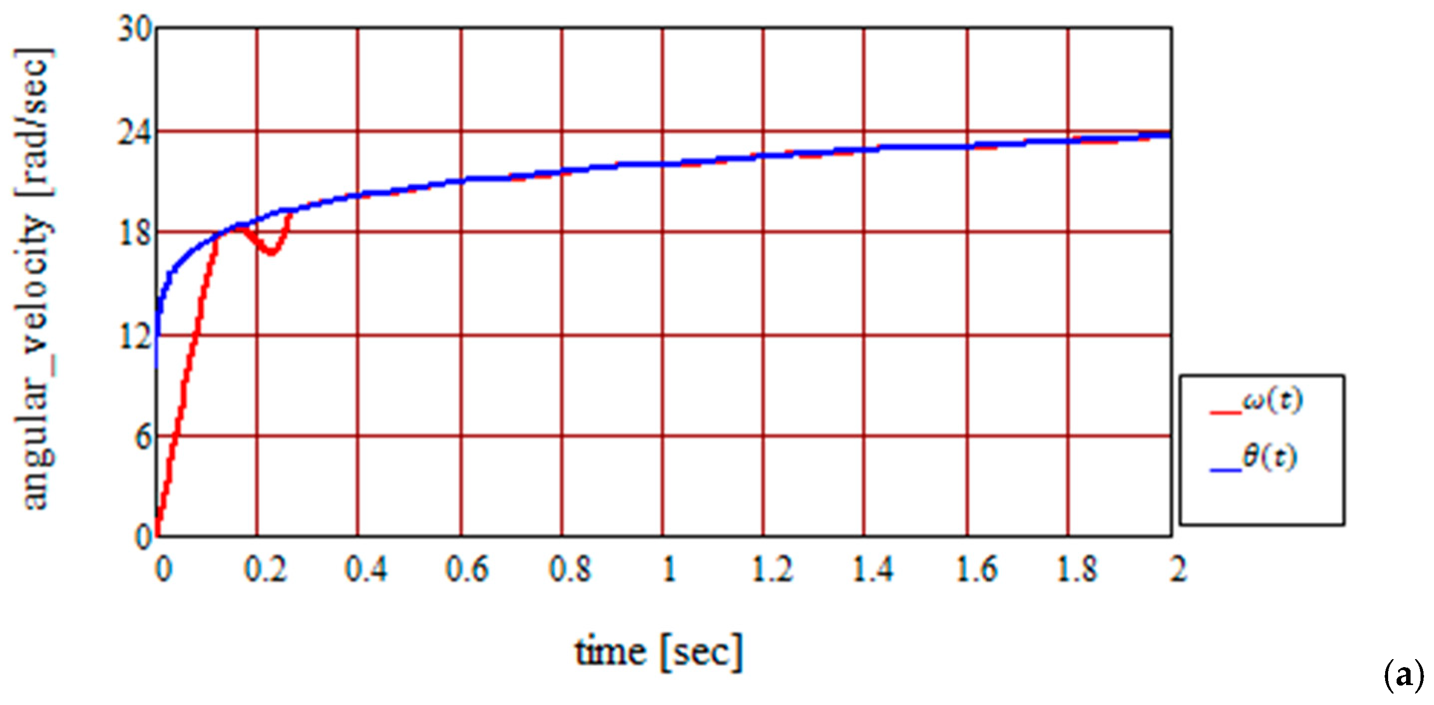
• Laws of motion of the ring $\theta =\theta \left(t\right)$;
• Other characteristics: coefficients of friction ${{\mu }^{\prime }}_s$, ${{\mu }^{″}}_s$, ${{\mu }^{\prime }}_k$, ${{\mu }^{″}}_k$; ratio $\Delta \theta /(\pi -\Delta \theta$) between the dimensions of the two regions with different coefficients of friction; velocity of transition from static to dynamic friction regime $v_0$.

The model presented in this study can be applied to other more complex dynamic systems where rotation motion about a well-specified axis is present and where, on the contact regions, there are discontinuities in the variations of the dynamic friction coefficient. To be more specific, for the systems characterised by the fact that in all contact points from the contact region, the same relative velocity vector exists. The model cannot be applied for dynamic systems that contain pairs with more degrees of freedom where the relative velocity is variable at different points of the contact region.

4. Conclusions

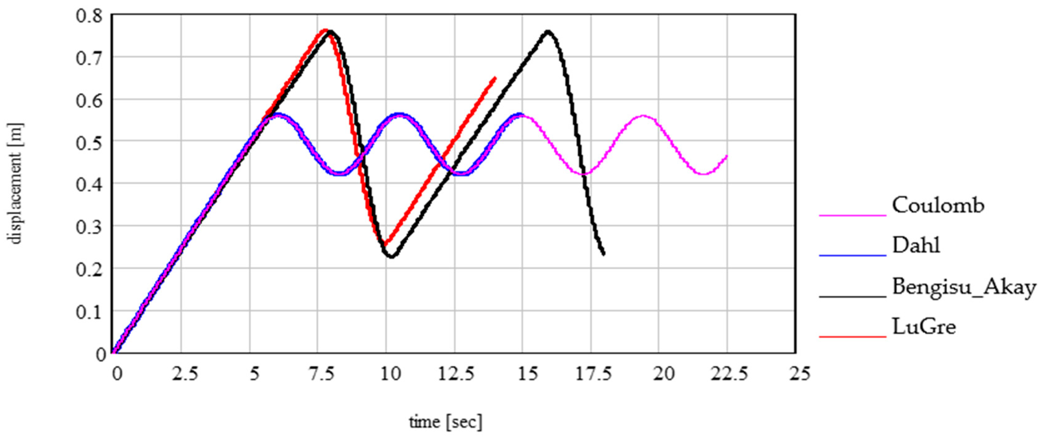
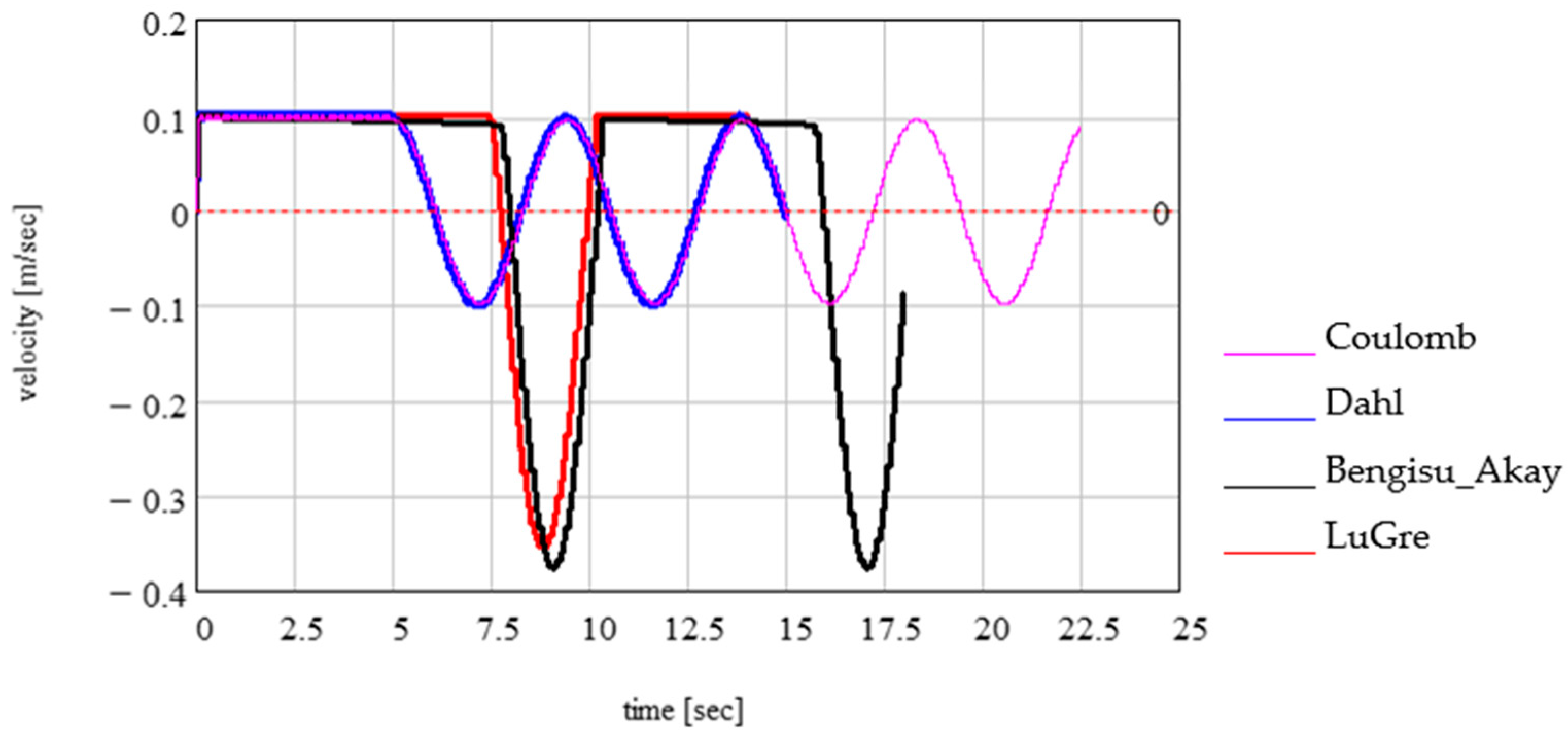
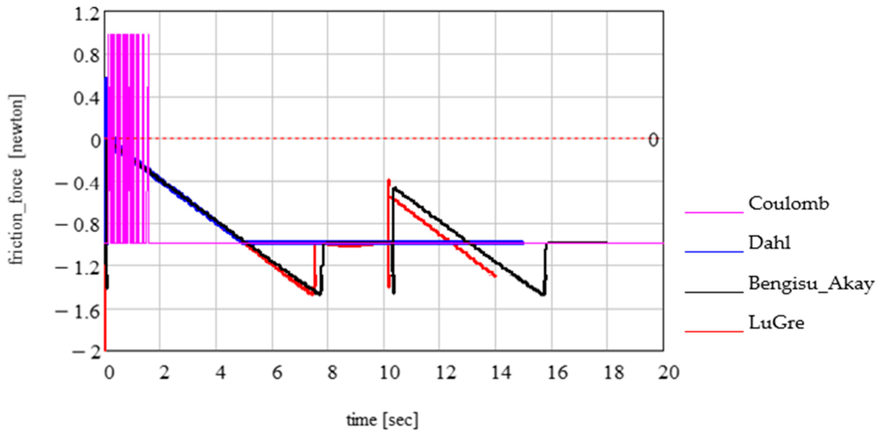
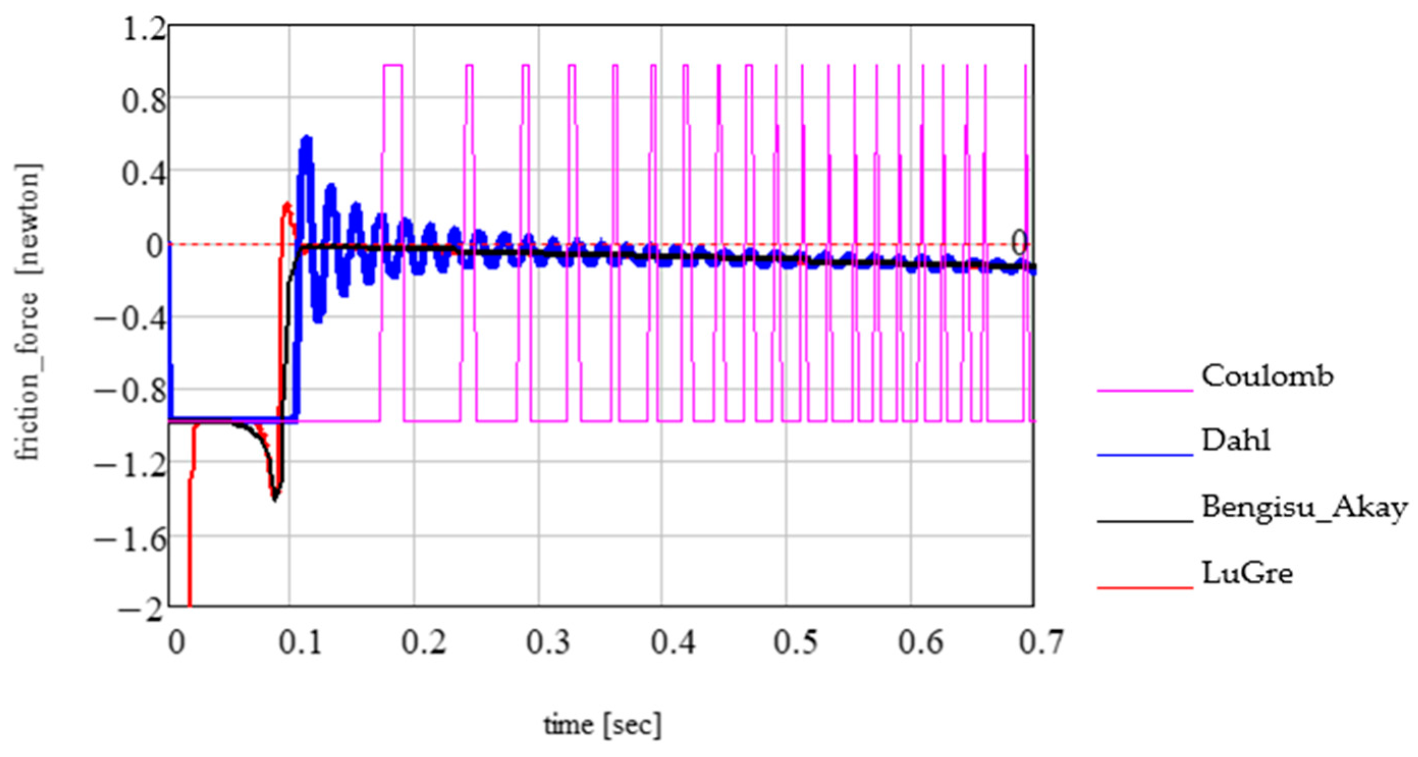
• In the introductory section, we presented a few widely known friction models; then, four of the models (Coulomb, Bengisu–Akay, Dahl, and LuGre) were analysed for a recognised dynamic system for unidirectional motion: a body on a mobile rough conveyor belt elastically coupled to the ground via a spring.
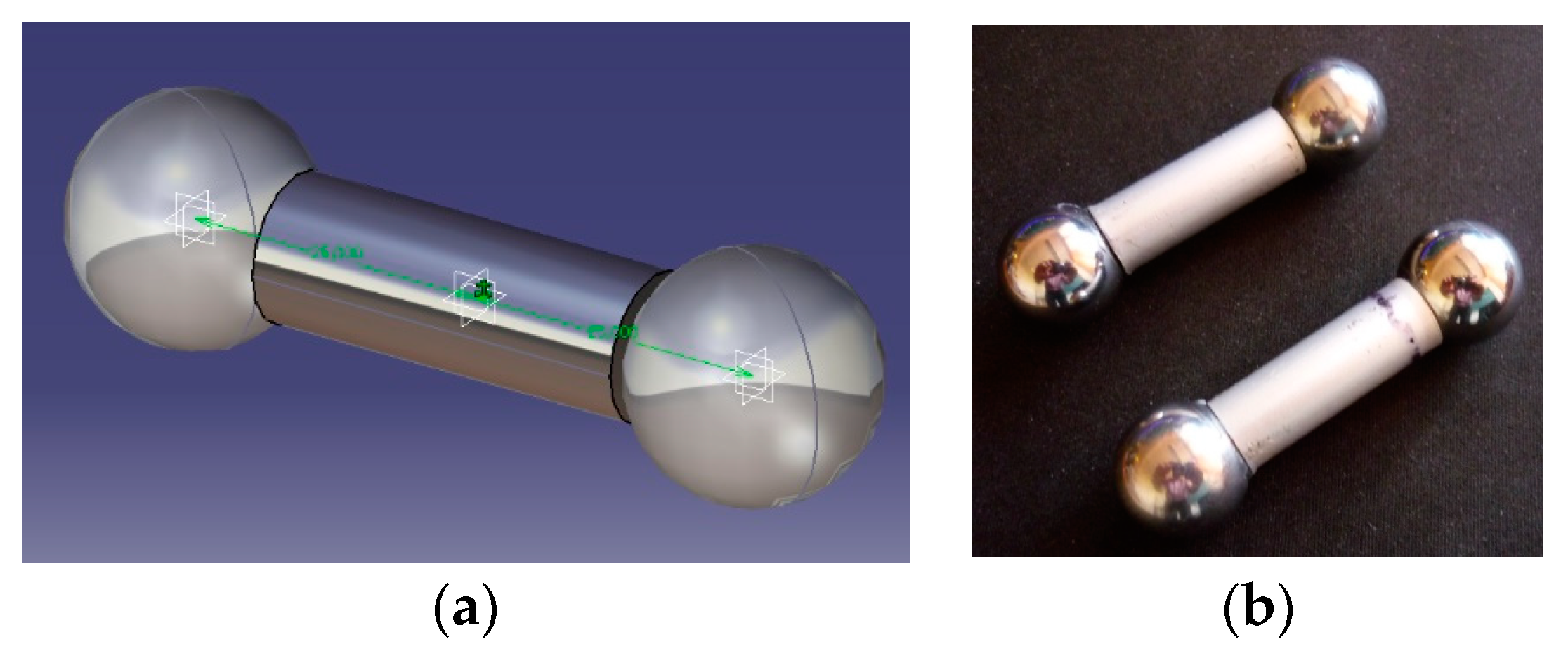
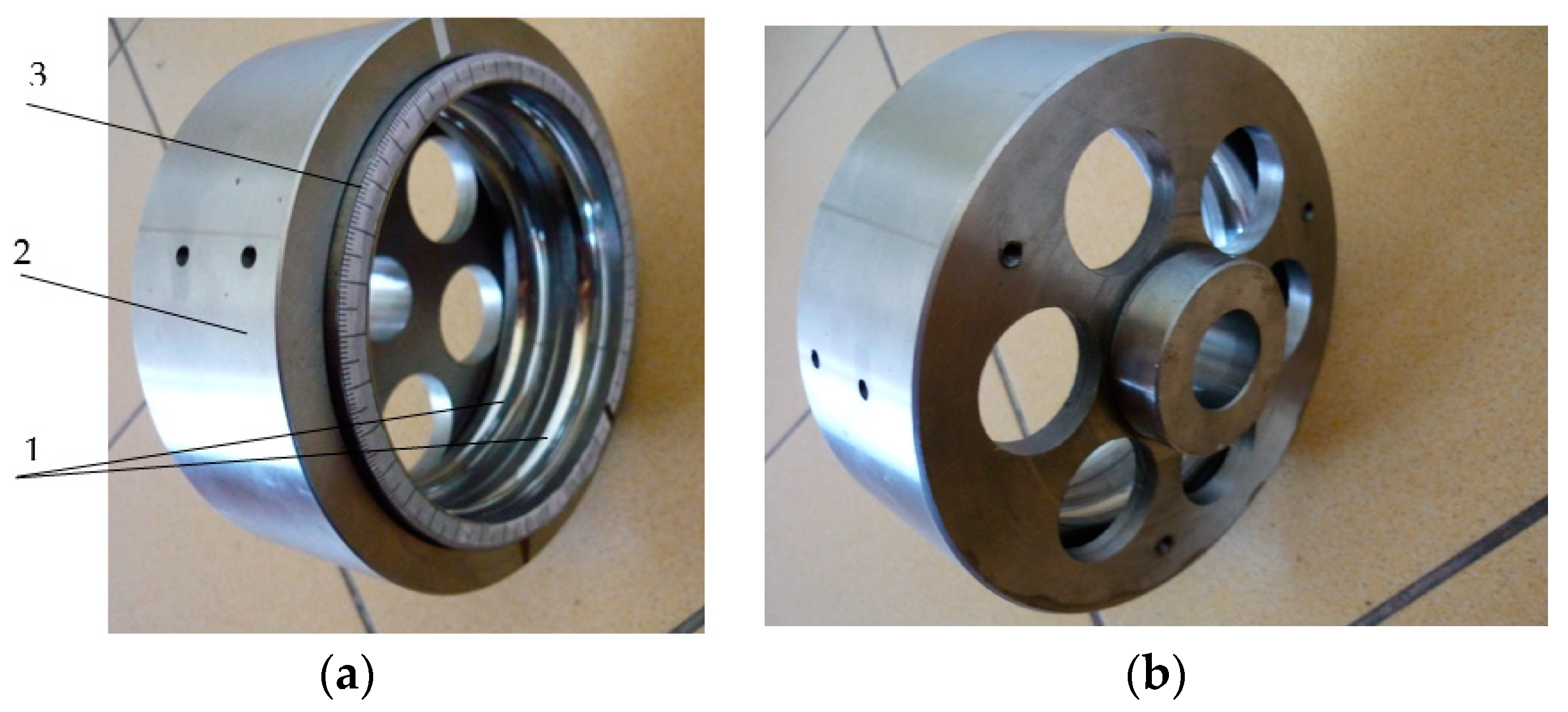
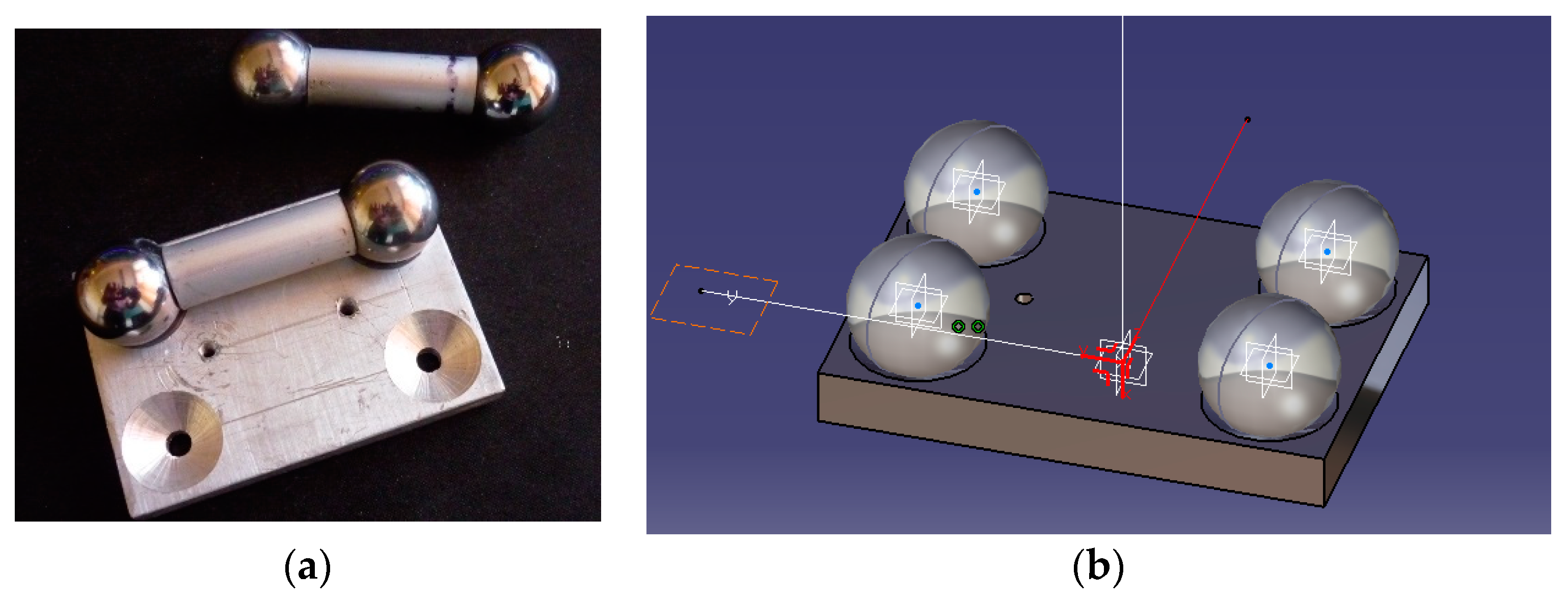
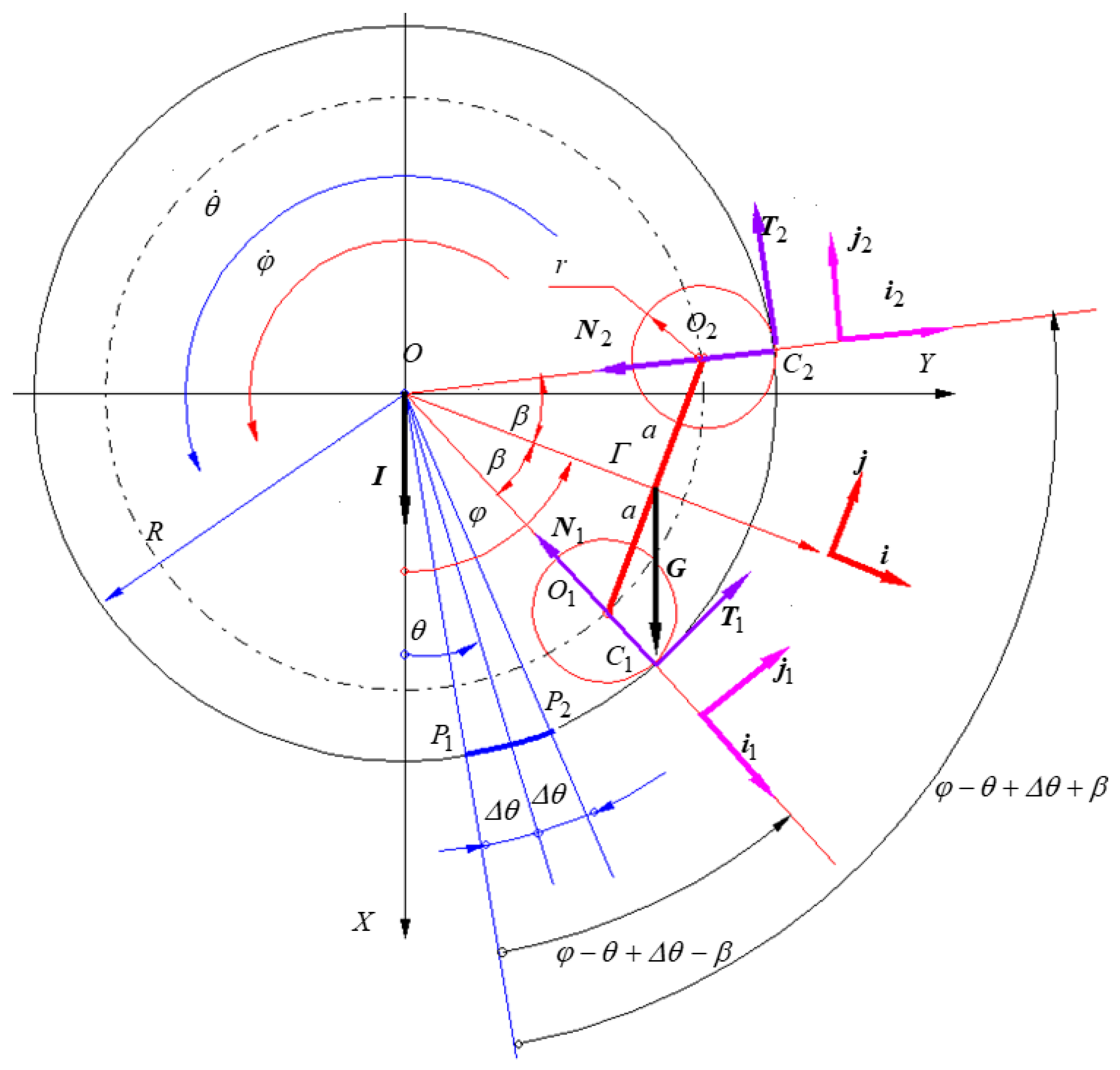
• We proposed a mathematical model for a dynamic system with dry friction. Two identical balls connected by a rod, contacting the inner surface of a metallic cylinder that rotates about a horizontal axis, obey a known law. The surface of the cylinder presents regions with different roughnesses.
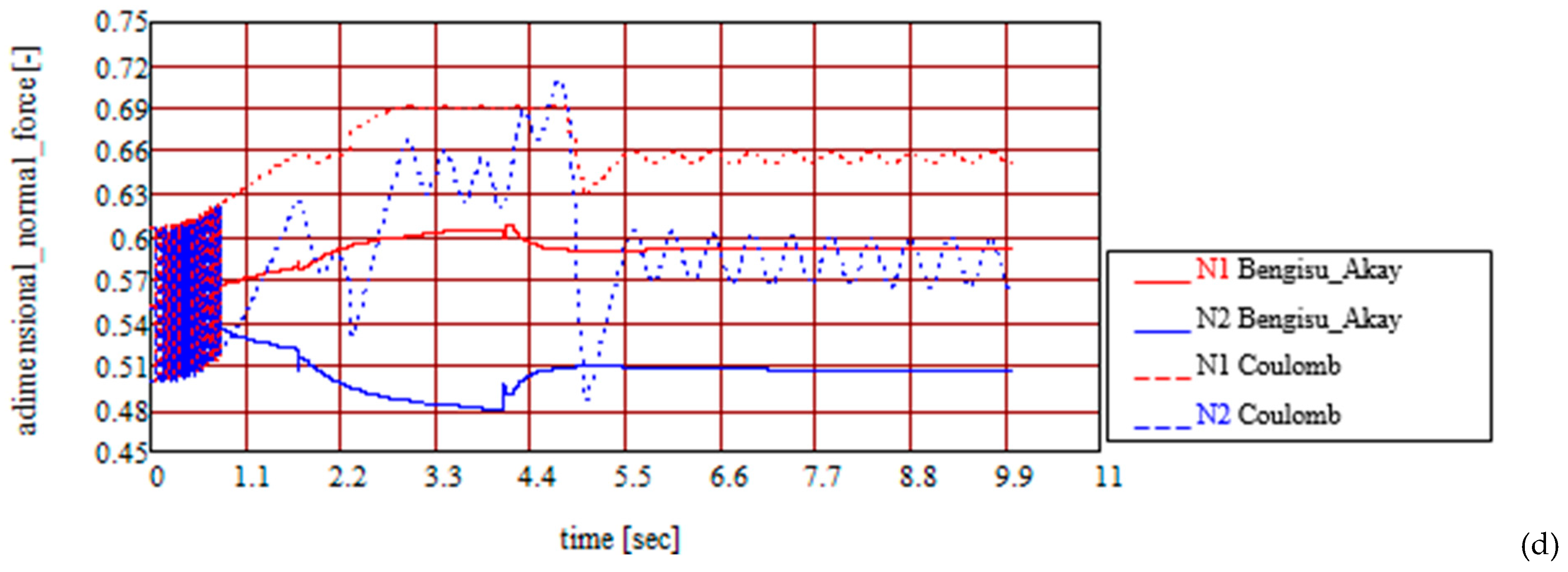
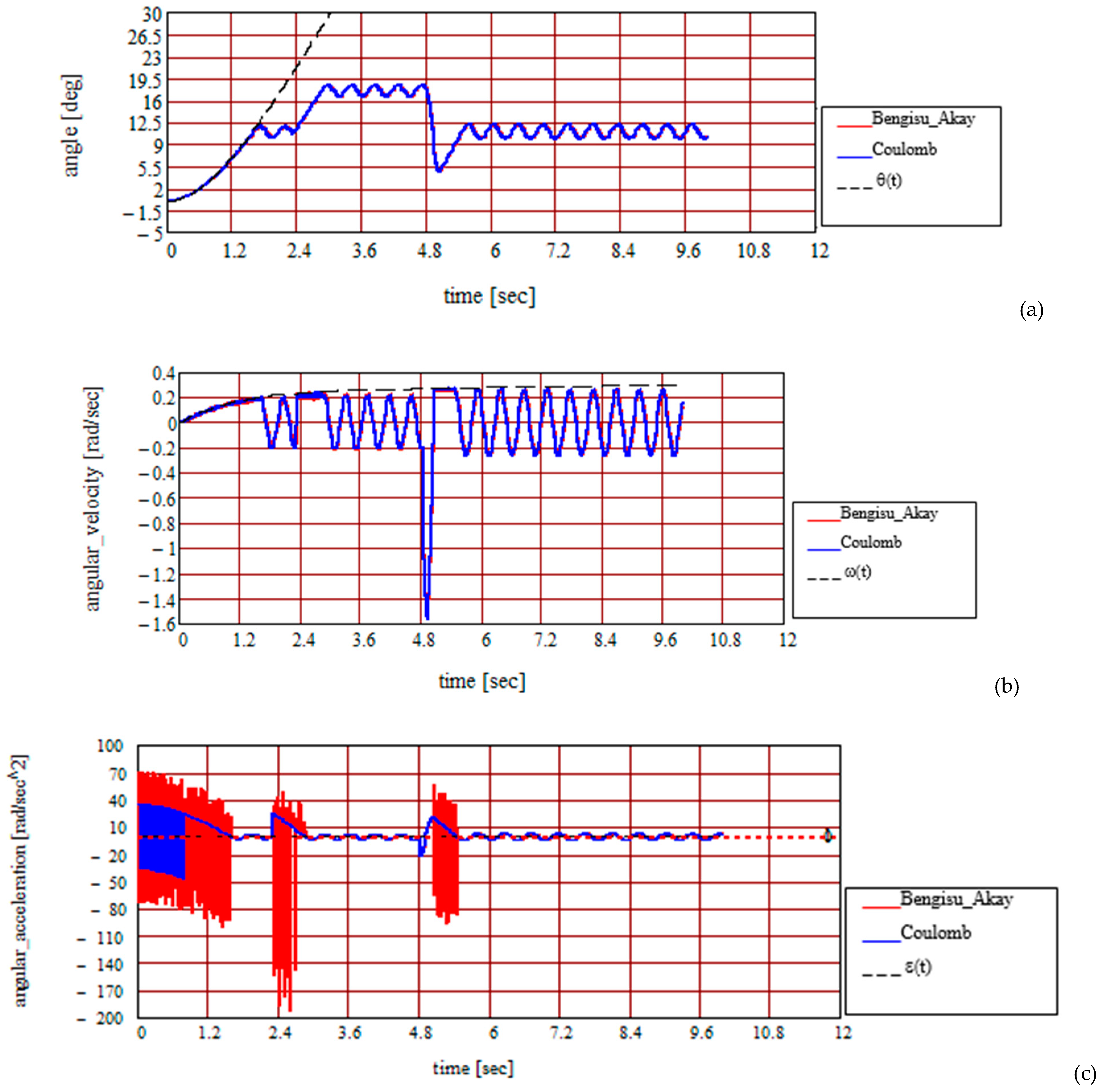
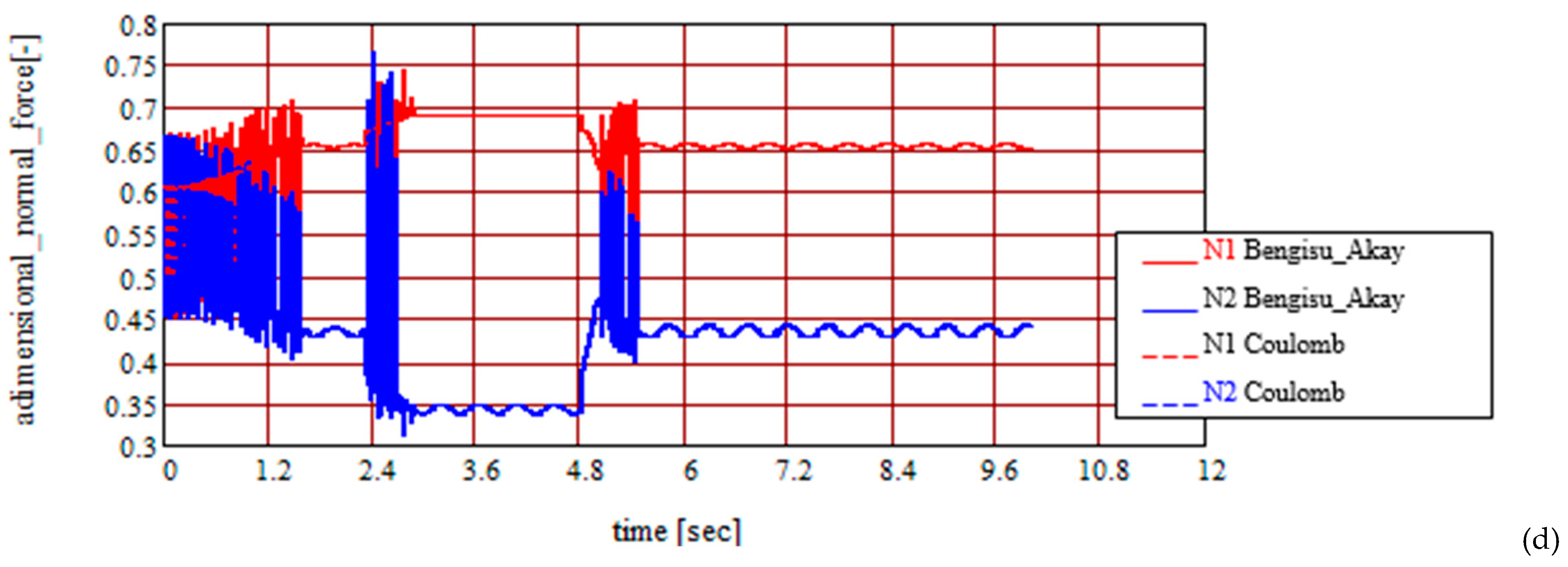
• The unknowns of the problem of the body performing plane-parallel motion are the position angle of the axis of symmetry of the mobile body and the magnitudes of the normal reactions from the contact points.
• An important subject is adopting the dry friction model for the ball–ring contact points: the Coulomb and Bengisu–Akay models were adopted because both these models consider the proportionality between the friction force and magnitude of the normal reaction, a fact that substantially simplifies the calculus for obtaining and integrating the equations of motion for the new model.
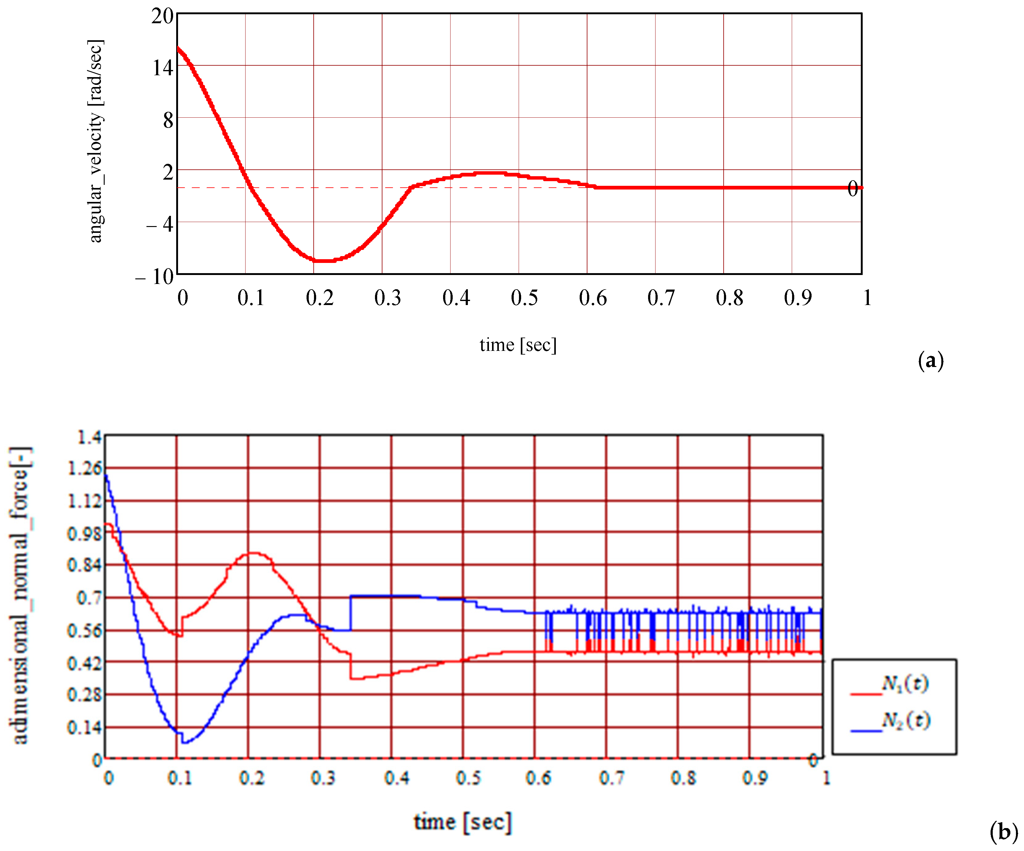
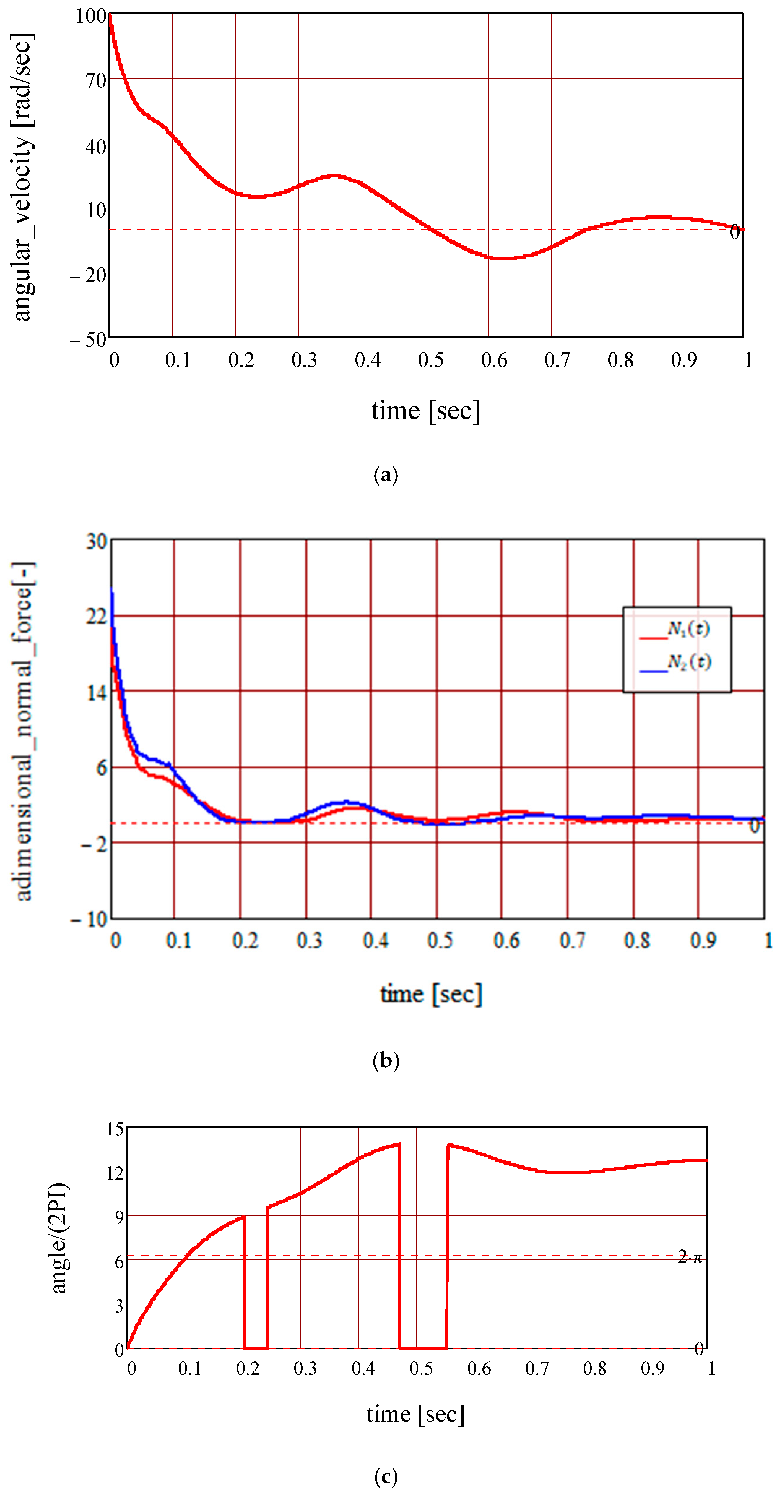
• The proposed dynamic model highlights the following phenomena, depending on the law of motion of the ring:
• Moving ring: oscillatory motion without separation (detachment); oscillatory motion with separation; circular motion without separation;
• Immobile ring and the body launched into motion: oscillatory damped motion; oscillatory motion with detachment; circular motion with separation;
• Future research aims at quantitative corroboration, besides the qualitative validation in the presented experimental findings, consisting in obtaining the laws of motion of the ring and of the body, using a device based on modern measurement techniques.

References

1. Duca, C.; Buium, F.; Paraoaru, G. Mechanisms (Mecanisme, in Romanian); Gheorghe Asachi: Iasi, Romania, 2003; pp. 277–285. [Google Scholar]
2. Broch, J.T. Mechanical Vibrations and Shock Measurements, 2nd ed.; Bruel and Kjaer: Naerum, Denmark, 1984; pp. 72–83. [Google Scholar]
3. Marques, F.; Flores, P.; Claro, J.C.; Lankarani, H. A survey and comparison of several friction force models for dynamic analysis of multibody mechanical systems. Nonlinear Dyn. 2016, 86, 1407–1443. [Google Scholar] [CrossRef]
4. Ronnie Hensen, A.H. Controlled Mechanical Systems with Friction. Ph.D. Thesis, Technische Universiteit Eindhoven, Eindhoven, The Netherlands, 21 February 2002. [Google Scholar]
5. Pfeiffer, F.; Glocker, C. Multibody Dynamics with Unilateral Contacts; John Wiley & Sons: Hoboken, NJ, USA, 1996; pp. 51–69. [Google Scholar]
6. Ardema, M.D. Newton-Euler Dynamics; Springer: New York, NY, USA, 2006; pp. 231–260. ISBN 978-0-387-23276-8. [Google Scholar]
7. Khan, Z.; Chacko, V.; Nazir, H. A review of friction models in interacting joints for durability design. Friction 2017, 5, 1–22. [Google Scholar] [CrossRef]
8. Pennestri, E.; Rossi, V.; Salvini, P.; Valentini, P.P. Review and comparison of dry friction force models. Nonlinear Dyn. 2016, 83, 1785–1801. [Google Scholar] [CrossRef]
9. Pennestrì, E.; Valentini, P.P.; Vita, L. Multibody dynamics simulation of planar linkages with Dahl friction. Multibody Syst. Dyn. 2007, 17, 321–347. [Google Scholar] [CrossRef]
10. Amontons, G. De la resistance cause’e dans les machines. Mém. l’Academie R. A. 1699, 257–282. [Google Scholar]
11. Coulomb, C.A. Théorie des Machines Simples, en Ayant Égard au Frottement de Leurs Parties, et à la Roideur des Cordages; Bachelier, Libraire: Paris, France, 1821; pp. 212–245. [Google Scholar]
12. Taylor, R.I. Rough Surface Contact Modelling—A Review. Lubricants 2022, 10, 98. [Google Scholar] [CrossRef]
13. Greenwood, J.A.; Williamson, J.B.P. Contact of Nominally Flat Surfaces. Proc. R. Soc. Lond. Ser. A Math. Phys. Sci. 1966, 295, 300–319. [Google Scholar]
14. Greenwood, J.; Tripp, J. Contact of two nominally flat rough surfaces. Proc. IMechE J. Mech. Eng. Sci. 1970, 185, 625–633. [Google Scholar] [CrossRef]
15. Leighton, M.; Morris, N.; Rahmani, R.; Rahnejat, H. Surface specific asperity model for prediction of friction in boundary and mixed regimes of lubrication. Meccanica 2017, 52, 21–33. [Google Scholar] [CrossRef]
16. Centea, D.; Rahnejat, H.; Menday, M.T. The influence of the interface coefficient of friction upon the propensity to judder in automotive clutches. Proc. IMechE Part D J. Automob. Eng. 1999, 213, 245–258. [Google Scholar] [CrossRef]
17. Abinowicz, E. The nature of the static and kinetic coefficients of friction. J. Appl. Phys. 1951, 22, 1373–1379. [Google Scholar] [CrossRef]
18. Rabinowicz, E. Stick and slip. Sci. Am. 1956, 194, 109–118. [Google Scholar] [CrossRef]
19. Berger, E.J.; Mackin, T.J. On the walking stick-slip problem. Tribol. Int. 2014, 75, 51–60. [Google Scholar] [CrossRef]
20. Hess, D.P.; Soom, A. Friction at a lubricated line contact operating at oscillating sliding velocities. J. Tribol. 1990, 112, 147–152. [Google Scholar] [CrossRef]
21. Bo, L.C.; Pavelescu, D. The friction-speed relation and its influence on the critical velocity of stick-slip motion. Wear 1982, 82, 277–289. [Google Scholar]
22. Threlfall, D.C. The inclusion of Coulomb friction in mechanisms programs with particular reference to DRAM au programme DRAM. Mech. Mach. Theory 1973, 13, 475–483. [Google Scholar] [CrossRef]
23. Andersson, S.; Söderberg, A.; Björklund, S. Friction models for sliding dry, boundary and mixed lubricated contacts. Tribol. Int. 2007, 40, 580–587. [Google Scholar] [CrossRef]
24. Karnopp, D. Computer simulation of stick-slip friction in mechanical dynamic systems. J. Dyn. Syst. Meas. Control 1985, 107, 100–103. [Google Scholar] [CrossRef]
25. Bengisu, M.T.; Akay, A. Stability of friction-induced vibrations in multi-degree-of-freedom systems. J. Sound Vibr. 1994, 171, 557–570. [Google Scholar] [CrossRef]
26. Dahl, P.R. A Solid Friction Model-Technical Report; The Aerospace Corporation: El Segundo, CA, USA, 1968. [Google Scholar]
27. Dahl, P.R. Solid friction damping in mechanical vibrations. AIAA J. 1976, 14, 1675–1682. [Google Scholar] [CrossRef]
28. Haessig, D.A., Jr.; Friedland, B. On the modeling and simulation of friction. J. Dyn. Sys. Meas. Control 1991, 113, 354–362. [Google Scholar] [CrossRef]
29. Olsson, H.; Åström, K.J.; Canudas de Wit, C.; Gäfvert, M.; Lischinsky, P. Friction models and friction compensation. Eur. J. Control 1998, 4, 176–195. [Google Scholar] [CrossRef]
30. Armstrong-Hélouvry, B.; Dupont, P.; de Wit Canudas, C. A survey of models, analysis tools and compensation methods for the control of machines with friction. Automatica 1994, 30, 1083–1138. [Google Scholar] [CrossRef]
31. Canudas de Wit, C.; Olsson, H.; Åström, K.J.; Lischinsky, P. A new model for control of systems with friction. IEEE Trans. Autom. Control 1995, 40, 419–425. [Google Scholar] [CrossRef]
32. Lenoir, Y. Identification des modèles tribologique par pendule. C. R. Acad. Sci. Ser. IIb Mec. Phys. Astron. 1999, 327, 1259–1264. [Google Scholar] [CrossRef]
33. Kermani, M.R.; Pate, R.V. Friction Identification in Robotic Manipulators, Case Studies. In Proceedings of the IEEE Conference on Control Applications, Toronto, ON, Canada, 28–31 August 2005. [Google Scholar]
34. Arnoux, J.J.; Sutter, G.; List, G.; Molinari, A. Friction experiments for dynamical coefficient measurement. Adv. Tribol. 2011, 1, 1–6. [Google Scholar] [CrossRef]
35. Dupont, P.; Armstrong, B.; Hayward, V. Elasto-plastic friction model: Contact compliance and stiction. In Proceedings of the American Control Conference, Chicago, IL, USA, 28–30 June 2000. [Google Scholar]
36. Dupont, P.; Hayward, V.; Armstrong, B.; Altpeter, F. Single state elasto-plastic friction models. IEEE Trans. Autom. Control 2002, 47, 787–792. [Google Scholar] [CrossRef]
37. Atkinson, K.; Han, W.; Stewart, D. Numerical Solution of Ordinary Differential Equations; John Wiley & Sons: Hoboken, NJ, USA, 2009; pp. 67–94. [Google Scholar]
38. Butcher, J.C. Numerical Methods for Ordinary Differential Equations, 2nd ed.; John Wiley & Sons: Chichester, UK, 2008; pp. 93–104. [Google Scholar]
39. Ciornei, F.C.; Diaconescu, E. Dynamic contact between a rigid indenter and a Kelvin-Voigt half-space. In Proceedings of the World Tribology Congress III, Washington, DC, USA, 12–16 September 2005. [Google Scholar]
40. Ciornei, F.C.; Alaci, S.; Bujoreanu, C. A model of the effect of dry friction on the behaviour of a dynamical system. IOP Conf. Ser. Mater. Sci. Eng. 2020, 997, 012006. [Google Scholar] [CrossRef]
41. Maxfield, B. Engineering with Mathcad; Elsevier Linacre House: Oxford, UK, 2006; pp. 317–335. [Google Scholar]
42. Moore, H. MATLAB for Engineers, 6th ed.; Pearson Education Inc.: Hoboken, NJ, USA, 2022; pp. 59–102. [Google Scholar]
43. Zamani, N.; Weaver, G.M. CATIA V5 Tutorials Mechanism Design & Animation, 1st ed.; SDC Publications: Mission, KS, USA, 2012. [Google Scholar]
Figure 1. Device for the study of the effects of friction force in a 1DOF system.
Computation 12 00181 g001
Figure 2. Coulomb friction model.
Computation 12 00181 g002
Figure 3. Coulomb friction with stiction.
Computation 12 00181 g003
Figure 4. The Karnopp [24] friction model.
Computation 12 00181 g004
Figure 5. Regularisation of the friction force with stiction.
Computation 12 00181 g005
Figure 6. Smoothened solution for friction with stiction.
Computation 12 00181 g006
Figure 7. The friction force modelled according to Bengisu and Akay [25].
Computation 12 00181 g007
Figure 8. The bristle model for friction force.
Computation 12 00181 g008
Figure 9. The displacements of the body for the four friction models.
Computation 12 00181 g009
Figure 10. The velocities of the body for the four friction models.
Computation 12 00181 g010
Figure 11. The variations in the friction force for the four friction models.
Computation 12 00181 g011
Figure 12. Details of the variations in the friction force immediately after the start of motion for the four friction models.
Computation 12 00181 g012
Figure 13. The proposed model for the dynamic system.
Computation 12 00181 g013
Figure 14. Designed (a) and manufactured (b) mobile bodies.
Computation 12 00181 g014
Figure 15. Ensuring the co-axiality of the bearing rings using the driving part: outer bearing rings 1, driving part 2, angular scale 3; (a) front view; (b) back view.
Computation 12 00181 g015
Figure 16. Solutions for oscillating body: (a) two rods with balls fixed on a plate; (b) four balls fixed on a plate.
Computation 12 00181 g016
Figure 17. The experimental device: (a) design; (b) manufactured device.
Computation 12 00181 g017
Figure 18. Finding the motion of the ring: (a) filming with a high-speed camera; (b) film split into frames for identifying the extreme positions of the mobile body.
Computation 12 00181 g018
Figure 19. Angular amplitudes of the mobile body.
Computation 12 00181 g019
Figure 20. Extreme positions of oscillating bodies: right (a) and left (b) extremes for the first configuration; right (c) and left (d) extremes for the second configuration, with interchanged mobile bodies.
Computation 12 00181 g020
Figure 21. Surface of the back ring: (a) presence of wear on the race; (b) detail of the race wear (scratch).
Computation 12 00181 g021
Figure 22. Theoretical dynamic model of the system.
Computation 12 00181 g022
Figure 23. Representation of the function ψ x , with bold red line. The extreme values are marked with the dashed red lines.
Computation 12 00181 g023
Figure 24. The inertial characteristics of the system: (a) model from CATIA; (b) inertial characteristics provided by CATIA; (c) scaling the mass of the actual body.
Computation 12 00181 g024
Figure 25. Variations with time for the imposed parameters μ s = 0.5 ; μ k = 0.3 ; μ s = 0.3 ; μ k = 0.1 ;   α = 100   s / m ;   0.2   m / s ; Δ θ = 15 ; φ 0 = 0   r a d / s ; Δ t = 10 ; n = 15,000 , and the law of motion θ ( t ) = 0.2 [ t · atan t 0.5 ln ( 1 + t 2 ) ] of (a) the angle φ , (b) angular velocity ω , (c) angular acceleration ε , (d) normal reactions N 1 and N 2 .
Computation 12 00181 g025
Figure 26. Variations with time for the imposed parameters μ s = 0.5 ; μ k = 0.3 ; μ s = 0.2 , μ k = 0.1 ;   α = 100   s / m ; v 0 = 20 × 10 6   m / s , Δ θ = 1 5 ; ϕ 0 = 0 ;   ω 0 = 0 ; Δ t = 10 , n = 15,000 ; θ ( t ) = 0.2 [ t · a t a n t 0.5 ln ( 1 + t 2 ) ] of (a) angle φ , (b) angular velocity ω , (c) angular acceleration ε , (d) normal reactions N 1 and N 2 .
Computation 12 00181 g026
Figure 27. Variations with time for the imposed parameters μ s = 0.5 , μ k = 0.3 , μ s = 0.2 , μ k = 0.1 α = 10 4   s / m , v 0 = 0.2   m / s , Δ θ = 15 , ϕ 0 = 0 , ω 0 = 0 , Δ t = 10 , n = 15,000 , θ ( t ) = 0.2 [ t · atan t 0.5 ln ( 1 + t 2 ) ] of (a) angle φ , (b) angular velocity ω , (c) angular acceleration ε , (d) normal reactions N 1 and N 2 .
Computation 12 00181 g027aComputation 12 00181 g027b
Figure 28. Variations with time for the imposed parameters μ s = 0.5 , μ k = 0.3 , μ s = 0.2 , μ k = 0.1 α = 10 4   s / m , v 0 = 2 × 10 6   m / s , Δ θ = 15 , ϕ 0 = 0 , ω 0 = 0 , Δ t = 10 , n = 15,000 , θ ( t ) = 0.2 [ t · atan t 0.5 ln ( 1 + t 2 ) ] of (a) angle φ ; (b) angular velocity ω ; (c) angular acceleration ε ; (d) normal reactions N 1 and N 2 .
Computation 12 00181 g028aComputation 12 00181 g028b
Figure 29. Dynamic system excited to oscillatory motion ( ω presents change in sense) with no separation ( N 1 > 0 , N 2 > 0 ), μ s = 0.5 , μ k = 0.3 , μ s = 0.2 , μ k = 0.1 α = 10 5   s / m , 2 × 10 6   m / s , Δ θ = 15 , ϕ 0 = 0 ,   ω 0 = 0 ,   Δ t = 10 ,   n = 5000 ,   θ ( t ) = 2 [ t · atan t 0.5 ln ( 1 + t 2 ) ] ; (a) angular velocity ω ; (b) normal reactions N 1 and N 2 .
Computation 12 00181 g029
Figure 30. Dynamic system excited to oscillatory motion ( ω presents change in sense) with separation, N 1 > 0 ( N 2 has changed sign) μ s = 0.5 , μ k = 0.3 , μ s = 0.2 , μ k = 0.1 , α = 10 5   s / m , v 0 = 2 × 10 6   m / s , Δ θ = 15 , ϕ 0 = 0 , ω 0 = 0   r a d / s , Δ t = 8 , n = 15,000 , θ ( t ) = 10 [ t · atan t 0.5 ln ( 1 + t 2 ) ] ; (a) angular velocity ω ; (b) normal reactions N 1 and N 2 .
Computation 12 00181 g030
Figure 31. Dynamic system excited to circular motion ( ω maintains unchanged sign), without separation ( N 1 > 0 , N 2 > 0 ) μ s = 0.5 , μ k = 0.4 , μ s = 0.2 , μ k = 0.1 α = 10 5   s / m , v 0 = 2 × 10 6   m / s , Δ θ = 90 , ϕ 0 = 0   r a d / s , ω 0 = 0   r a d / s   Δ t = 2 , n = 5000 , θ ( t ) = 20 · t 1.1 ; (a) angular velocity ω ; (b) normal reactions N 1 and N 2 .
Computation 12 00181 g031aComputation 12 00181 g031b
Figure 32. Dynamic system excited to oscillatory motion ( ω has a shift in signum), without separation ( N 1 > 0 , N 2 > 0 ), μ s = 0.2 , μ k = 0.15 , μ s = 0.15 , μ k = 0.1 α = 10 5   s / m , v 0 = 2 × 10 6   m / s , Δ θ = 15 , ϕ 0 = 0 , ω 0 = 16   r a d / s , Δ t = 1 , n = 5000 , θ ( t ) = 0 ; (a) angular velocity ω ; (b) normal reactions N 1 and N 2 .
Computation 12 00181 g032
Figure 33. Dynamic system excited to circular motion ( ω maintains unchanged sign), with separation ( N 1 > 0 , N 2 < 0 ,   s i g n u m   s h i f t ) μ s = 0.2 , μ k = 0.15 , μ s = 0.15 , μ k = 0.1 α = 10 5   s / m , v 0 = 2 × 10 6   m / s , Δ θ = 15 , ϕ 0 = 0 , ω 0 = 100   r a d / s , Δ t = 1 , n = 5000 , θ ( t ) = 0 ; (a) angular velocity ω ; (b) normal reactions N 1 and N 2 ; (c) position angle.
Computation 12 00181 g033
Disclaimer/Publisher’s Note: The statements, opinions and data contained in all publications are solely those of the individual author(s) and contributor(s) and not of MDPI and/or the editor(s). MDPI and/or the editor(s) disclaim responsibility for any injury to people or property resulting from any ideas, methods, instructions or products referred to in the content.